Time Delay Systems Part 9 pot
Bạn đang xem bản rút gọn của tài liệu. Xem và tải ngay bản đầy đủ của tài liệu tại đây (421.95 KB, 20 trang )
Now, let r
5
be a positive scalar, then using Fact 1 we have
−2x
(t)PA
d
0
−τ
μ(t + s)B
o
Ix(t + s)ds = −2x
(t)PA
d
0
−τ
B
o
Iz(t + s)ds
≤ τ
+
r
−1
5
x
(t)PA
d
A
d
Px(t)+r
5
0
−τ
z
(t + s)I
B
o
B
o
Iz(t + s)ds. (35)
Also, if r
6
is a positive scalar, then using Fact 1 we have
−2x
(t)PA
d
0
−τ
E(x, t + s)ds ≤ τ
+
r
−1
6
x
(t)PA
d
A
d
Px(t)
+
r
6
0
−τ
E
(x, t + s)E(x, t + s)ds. (36)
It is known that
2μ(t)x
(t)PB
o
Ix(t) ≤ 2||PB
o
I|||μ(t) |||x(t)||
2
. (37)
Also, using Assumption 2.1, it can be shown that
2x
(t)PE(x, t) ≤ 2||P|| θ
∗
||x(t)||
2
. (38)
Using equations (31)- (38) and equations (17)- (24) (with the fact that 0
≤ τ ≤ τ
+
) in (30), we
have
˙
V
a
(x) ≤ x
(t)Ξ x(t)+τ
+
r
4
x
(t)ΔK
(t)B
o
B
o
ΔK(t)x(t)
+
τ
+
r
5
z
(t)I
B
o
B
o
Iz(t)+τ
+
r
6
E
(x, t)E(x, t)+2ρ
∗
||PB
o
|| ||x(t)||
2
+2||PB
o
I|||μ(t)|||x(t) ||
2
+ 2θ
∗
||P|| ||x(t)||
2
+ 2 μ(t)
˙
μ
(t). (39)
where
Ξ = PA
od
+ A
od
P + PB
o
K + K
B
o
P + τ
+
r
1
A
o
A
o
+ τ
+
r
2
A
d
A
d
+ τ
+
r
3
B
o
KK
B
o
+τ
+
r
−1
1
+ r
−1
2
+ r
−1
3
+ r
−1
4
+ r
−1
5
+ r
−1
6
PA
d
A
d
P. (40)
To guarantee that x
(t)Ξ x(t) < 0, it sufficient to show that Ξ < 0. Let us introduce the
linearizing terms,
X = P
−1
, Y = KX,andZ = XB
o
K. Also, let ε
1
= r
−1
1
, ε
2
= r
−1
2
, ε
3
= r
−1
3
,
ε
4
= r
−1
4
, ε
5
= r
−1
5
and ε
6
= r
−1
6
. Now, by pre-multiplying and post-multiplying Ξ by X and
invoking the Schur complement, we arrive at the LMI (25) which guarantees that Ξ
< 0, and
consequently x
(t)Ξ x(t) < 0. Now, we need to show that the remaining terms of (39) are
negative definite. Using the definition of z
(t)=μ(t)x(t), we know that
τ
+
r
5
z
(t)I
B
o
B
o
Iz(t) ≤ τ
+
r
5
||I
B
o
B
o
I||μ
2
(t) ||x(t)||
2
. (41)
Also, using Assumptions 2.1 and 2.2 , we have
τ
+
r
6
E
(x, t)E(x, t) ≤ τ
+
r
6
(
θ
∗
)
2
||x(t)||
2
, (42)
and
τ
+
r
4
x
(t)ΔK
(t)B
o
B
o
ΔK( t)x(t) ≤ τ
+
r
4
(
ρ
∗
)
2
||B
o
B
o
|| ||x(t)||
2
. (43)
149
Resilient Adaptive Control of Uncertain Time-Delay Systems
Now, using (41)- (43), the adaptive law (26), and the fact that |μ(t)|≥1, equation (39) becomes
˙
V
a
(x) ≤ x
(t)Ξ x(t)+τ
+
r
4
(
ρ
∗
)
2
||B
o
B
o
|| ||x(t)||
2
+ τ
+
r
5
||I
B
o
B
o
I||μ
2
(t) ||x(t)||
2
+τ
+
r
6
(
θ
∗
)
2
||x(t)||
2
+ 2ρ
∗
||PB
o
|| ||x(t)||
2
+ 2||PB
o
I|||μ(t) |||x(t)||
2
+2θ
∗
||P|| ||x(t)||
2
+ 2α
1
|μ(t)|||x(t)||
2
+ 2α
2
μ
2
(t) ||x(t)||
2
. (44)
It can be easily shown that by selecting α
1
and α
2
as in (27) and (28), we guarantee that
˙
V
a
(x) ≤ x
(t)Ξ x(t), (45)
where Ξ
< 0. Hence,
˙
V
a
(x) < 0 which guarantees asymptotic stabilization of the closed-loop
system.
3.2 Adaptive control when θ
∗
is known and ρ
∗
is unknown
Here, we wish to stabilize the system (6) considering the control law (3) when θ
∗
is known
and ρ
∗
is unknown. Before we present the stability results for this case, let us define
˜
ρ(t)=
ˆ
ρ
(t) −ρ
∗
,where
ˆ
ρ(t) is the estimate of ρ
∗
,and
˜
ρ(t) is error between the estimate and the true
value of ρ
∗
. Let the Lyapunov-Krasovskii functional for the transformed system (6) be selected
as:
V
b
(x)
Δ
= V
a
(x)+V
9
(x), (46)
where V
a
(x) is defined in equations (7), and V
9
(x) is defined as
V
9
(x)=
(
1 + ρ
∗
)[
˜
ρ
(t)
]
2
, (47)
where its time derivative is
˙
V
9
(x)=2
(
1 + ρ
∗
)
˜
ρ
(t)
˙
˜
ρ
(t). (48)
Since
˜
ρ
(t)=
ˆ
ρ
(t) −ρ
∗
,then
˙
˜
ρ(t)=
˙
ˆ
ρ
(t). Hence, equation (48) becomes
˙
V
9
(x)=2
(
1 + ρ
∗
)[
ˆ
ρ
(t) −ρ
∗
]
˙
ˆ
ρ
(t). (49)
The next Theorem provides the main results for this case.
Theorem 2: Consider system (6). If there exist matrices 0
< X = X
∈
n×n
, Y∈
m×n
,
Z∈
n×n
, and scalars ε
1
> 0, ε
2
> 0, ε
3
> 0, ε
4
> ε, ε
5
> ε and ε
6
> ε (where ε is an arbitrary
small positive constant) such that the LMI (25) has a feasible solution, and K
= YX
−1
,andμ(t) and
ˆ
ρ
(t) are adapted subject to the adaptive laws
˙
μ
(t)=Proj
[
β
1
sgn
(
μ(t)
)
+ β
2
μ(t)+ β
3
sgn
(
μ(t)
)
ˆ
ρ
(t)
]
||x(t)||
2
, μ(t)
(50)
˙
ˆ
ρ
(t)=γ ||x(t)||
2
, (51)
where Proj
{·} Krstic et al. (1995) is applied to ensure that |μ(t)|≥1 as follows:
μ
(t)=
⎧
⎨
⎩
μ
(t) if |μ(t)|≥1
1 if 0
≤ μ(t) < 1
−1 if −1 < μ(t) < 0,
and the adaptive law parameters are selected such that β
1
<
−
1
2
τ
+
r
6
(
θ
∗
)
2
+ 2 ||PB
o
I|| + 2θ
∗
||P||
, β
2
< −
1
2
τ
+
r
5
||I
B
o
B
o
I||, γ >
1
2
τ
+
r
4
||B
o
B
o
||,
150
Time-Delay Systems
β
3
< −γ,and
ˆ
ρ(0) > 1, then the control law (3) will guarantee asymptotic stabilization of the
closed-loop system.
Proof The time derivative of V
b
(x) is
˙
V
b
(x)=
˙
V
a
(x)+
˙
V
9
(x). (52)
Following the steps used in the proof of Theorem 1 and using equation (49), it can be shown
that
˙
V
b
(x) ≤ x
(t)Ξ x(t)+τ
+
r
4
(
ρ
∗
)
2
||B
o
B
o
|| ||x(t)||
2
+ τ
+
r
5
||I
B
o
B
o
I||μ
2
(t) ||x(t)||
2
+τ
+
r
6
(
θ
∗
)
2
||x(t)||
2
+ 2ρ
∗
||PB
o
|| ||x(t)||
2
+ 2||PB
o
I|||μ(t) |||x(t)||
2
+2θ
∗
||P|| ||x(t)||
2
+ 2 μ(t)
˙
μ
(t)+2
(
1 + ρ
∗
)[
ˆ
ρ
(t) −ρ
∗
]
˙
ˆ
ρ
(t), (53)
where Ξ is defined in equation (40). Using the linearization procedure and invoking the Schur
complement (as in the proof of Theorem 1), it can be shown that Ξ is guaranteed to be negative
definite whenever the LMI (25) has a feasible solution. Using the adaptive laws (50)- (51)
in (53) and the fact that
|μ(t)|≥1, we get
˙
V
b
(x) ≤ x
(t)Ξ x(t)+τ
+
r
4
(
ρ
∗
)
2
||B
o
B
o
|| ||x(t)||
2
+ τ
+
r
5
||I
B
o
B
o
I||μ
2
(t) ||x(t)||
2
+τ
+
r
6
(
θ
∗
)
2
||x(t)||
2
+ 2ρ
∗
||PB
o
|| ||x(t)||
2
+2||PB
o
I|||μ(t)|||x(t) ||
2
+ 2θ
∗
||P|| ||x(t)||
2
+2β
1
|μ(t)|||x(t)||
2
+ 2β
2
μ
2
(t) ||x(t)||
2
+ 2β
3
ˆ
ρ
(t) |μ(t)|||x(t)||
2
+ 2γ
ˆ
ρ(t) ||x(t)||
2
−2γρ
∗
||x(t)||
2
−2γρ
∗
ˆ
ρ
(t) ||x(t)||
2
−2γ
(
ρ
∗
)
2
||x(t)||
2
. (54)
Using the fact that
|μ(t)| > 1 and arranging terms of equation (54), it can be shown
that
˙
V
b
(x) < 0 if we select β
1
< −
1
2
τ
+
r
6
(
θ
∗
)
2
+ 2 ||PB
o
I|| + 2θ
∗
||P||
, β
2
<
−
1
2
τ
+
r
5
||I
B
o
B
o
I||,andβ
3
< −γ,whereγ needs to be selected to satisfy the following
two conditions:
γ
>
1
2
τ
+
r
4
||B
o
B
o
||, (55)
and
2
||PB
o
||−2γ + 2γ
ˆ
ρ(t) < 0. (56)
Hence, we need to select γ such that
γ
> max
1
2
τ
+
r
4
||B
o
B
o
|| ,
||PB
o
||
1 −
ˆ
ρ
(t)
. (57)
It is clear that when
ˆ
ρ
(t) > 1, we only need to ensure that γ >
1
2
τ
+
r
4
||B
o
B
o
||.Notethatfrom
equation (51),
ˆ
ρ
(t) > 1 can be easily ensured by selecting
ˆ
ρ(0) > 1andγ >
1
2
τ
+
r
4
||B
o
B
o
||
to guarantee that
ˆ
ρ(t) in equation (51) is monotonically increasing. Hence, we guarantee that
˙
V
b
(x) ≤ x
(t) Ξ x(t), (58)
where Ξ
< 0. Hence,
˙
V
b
(x) < 0 which guarantees asymptotic stabilization of the closed-loop
system.
151
Resilient Adaptive Control of Uncertain Time-Delay Systems
3.3 Adaptive control when θ
∗
is unknown and ρ
∗
is known
Here, we wish to stabilize the system (6) considering the control law (3) when θ
∗
is unknown
and ρ
∗
is known. Since θ
∗
is unknown, let us define
˜
θ(t)=
ˆ
θ
(t) − θ
∗
,where
ˆ
θ(t) is the
estimate of θ
∗
,and
˜
θ(t) is error between the estimate and the true value of θ
∗
. Also, let the
Lyapunov-Krasovskii functional for the transformed system (6) be selected as:
V
c
(x)
Δ
= V
a
(x)+V
10
(x), (59)
where
V
10
(x)=
(
1 + θ
∗
)
˜
θ
(t)
2
, (60)
where its time derivative is
˙
V
10
(x)=2
(
1 + θ
∗
)
˜
θ(t)
˙
˜
θ
(t),
= 2
(
1 + θ
∗
)
ˆ
θ
(t) −θ
∗
˙
ˆ
θ
(t). (61)
The next Theorem provides the main results for this case.
Theorem 3: Consider system (6). If there exist matrices 0
< X = X
∈
n×n
, Y∈
m×n
,
Z∈
n×n
, and scalars ε
1
> 0, ε
2
> 0, ε
3
> 0, ε
4
> ε, ε
5
> ε and ε
6
> ε (where ε is an arbitrary
small positive constant) such that the LMI (25) has a feasible solution, and K
= YX
−1
,andμ( t) is
adapted subject to the adaptive laws
˙
μ
(t)=Proj
δ
1
sgn
(
μ(t)
)
||x(t)||
2
+ δ
2
μ(t) ||x(t)||
2
+ δ
3
sgn
(
μ(t)
)
ˆ
θ(t) ||x(t)||
2
, μ(t)
,(62)
˙
ˆ
θ
(t)=κ ||x(t)||
2
, (63)
where Proj
{·} Krstic et al. (1995) is applied to ensure that |μ(t)|≥1 as follows
μ
(t)=
⎧
⎨
⎩
μ
(t) if |μ(t)|≥1
1 if 0
≤ μ(t) < 1
−1 if −1 < μ(t) < 0,
and the adaptive law parameters are selected such that δ
1
<
−
||PB
o
I||+ τ
+
r
4
(
ρ
∗
)
2
||B
o
B
o
||+ ρ
∗
||PB
o
||
, δ
2
< −
1
2
τ
+
r
5
||I
B
o
B
o
I||, δ
3
< −κ,
κ
>
1
2
τ
+
r
6
and
ˆ
θ(0) > 1, then the control law (3) will guarantee asymptotic stabilization of the
closed-loop system.
Proof The time derivative of V
c
(x) is
˙
V
c
(x)=
˙
V
a
(x)+
˙
V
10
(x). (64)
Following the steps used in the proof of Theorem 1 and using equation (61), it can be shown
that
˙
V
c
(x) ≤ x
(t)Ξ x(t)+τ
+
r
4
x
(t)ΔK
(t)B
o
B
o
ΔK( t)x(t)+τ
+
r
5
z
(t)I
B
o
B
o
Iz(t)
+
τ
+
r
6
E
(x, t)E(x, t)+2ρ
∗
||PB
o
|| ||x(t)||
2
+ 2||PB
o
I|||μ(t)|||x(t) ||
2
+2θ
∗
||P|| ||x(t)||
2
+ 2 μ(t)
˙
μ
(t)+2
(
1 + θ
∗
)
ˆ
θ
(t) − θ
∗
˙
ˆ
θ
(t), (65)
152
Time-Delay Systems
where Ξ is defined in equation (40). Using the linearization procedure and invoking the
Schur complement (as in the proof of Theorem 1), it can be shown that Ξ is guaranteed to
be negative definite whenever the LMI (25) has a feasible solution. Now, we need to show
that the remaining terms of (65) are negative definite. Using the definition of z
(t)=μ(t)x(t),
we know that
τ
+
r
5
z
(t)I
B
o
B
o
Iz(t) ≤ τ
+
r
5
||I
B
o
B
o
I||μ
2
(t) ||x(t)||
2
. (66)
Also, using Assumptions 2.1 and 2.2 , we have
τ
+
r
6
E
(x, t)E(x, t) ≤ τ
+
r
6
(
θ
∗
)
2
||x(t)||
2
, (67)
and
τ
+
r
4
x
(t)ΔK
(t)B
o
B
o
ΔK( t)x(t) ≤ τ
+
r
4
(
ρ
∗
)
2
||B
o
B
o
|| ||x(t)||
2
. (68)
Now, using (66)- (68), the adaptive laws (62)- (63), and the fact that
|μ(t)|≥1, equation (65)
becomes
˙
V
c
(x) ≤ x
(t)Ξ x(t)+τ
+
r
4
(
ρ
∗
)
2
||B
o
B
o
|| ||x(t)||
2
+ τ
+
r
5
||I
B
o
B
o
I||μ
2
(t) ||x(t)||
2
+τ
+
r
6
(
θ
∗
)
2
||x(t)||
2
+ 2ρ
∗
||PB
o
|| ||x(t)||
2
+ 2||PB
o
I|||μ(t)|||x(t) ||
2
6 + 2θ
∗
||P|| ||x(t)||
2
+ 2δ
1
|μ(t)|||x(t)||
2
+ 2δ
2
μ
2
(t) ||x(t)||
2
+2δ
3
|μ(t)|
ˆ
θ
(t) ||x(t)||
2
+ 2κ |μ(t)|
ˆ
θ
(t) ||x(t)||
2
−2κθ
∗
||x(t)||
2
+2κθ
∗
ˆ
θ(t) ||x(t)||
2
−2κ
(
θ
∗
)
2
||x(t)||
2
. (69)
It can be shown that
˙
V
c
(x) < 0 if the adaptive law parameters δ
1
, δ
2
,andδ
3
are selected as
stated in Theorem 3, and κ is selected to satisfy the following two conditions: κ
>
1
2
τ
+
r
6
and
||P||−κ + κ
ˆ
θ(t) < 0. Hence, we need to select κ such that
κ
> max
1
2
τ
+
r
6
,
||P||
1 −
ˆ
θ
(t)
. (70)
It is clear that when
ˆ
θ
(t) > 1, we only need to ensure that κ >
1
2
τ
+
r
6
.Notethatfrom
equation (63),
ˆ
θ
(t) > 1 can be easily ensured by selecting
ˆ
θ(0) > 1andκ >
1
2
τ
+
r
6
to
guarantee that
ˆ
θ
(t) in equation (63) is monotonically increasing. Hence, we guarantee that
˙
V
c
(x) ≤ x
(t)Ξ x(t), (71)
where Ξ
< 0. Hence,
˙
V
c
(x) < 0 which guarantees asymptotic stabilization of the closed-loop
system.
3.4 Adaptive control when both θ
∗
and ρ
∗
are unknown
Here, we wish to stabilize the system (6) considering the control law (3) when both θ
∗
and ρ
∗
are unknown. Here, the following Lyapunov-Krasovskii functional is used
V
d
(x)=V
c
(x)+V
11
(x), (72)
where V
c
(x) is defined in equations (59), and V
11
(x) is defined as
V
11
(x)=
(
1 + ρ
∗
)[
˜
ρ
(t)
]
2
, (73)
153
Resilient Adaptive Control of Uncertain Time-Delay Systems
where its time derivative is
˙
V
11
(x)=2
(
1 + ρ
∗
)
˜
ρ
(t)
˙
˜
ρ
(t). (74)
Since
˜
ρ
(t)=
ˆ
ρ
(t) −ρ
∗
,then
˙
˜
ρ(t)=
˙
ˆ
ρ
(t). Hence, equation (74) becomes
˙
V
11
(x)=2
(
1 + ρ
∗
)[
ˆ
ρ
(t) − ρ
∗
]
˙
ˆ
ρ
(t). (75)
The next Theorem provides the main results for this case.
Theorem 4: Consider system (6). If there exist matrices 0 < X = X
∈
n×n
, Y∈
m×n
,
Z∈
n×n
, and scalars ε
1
> 0, ε
2
> 0, ε
3
> 0, ε
4
> ε, ε
5
> ε and ε
6
> ε (where ε is an arbitrary
small positive constant) such that the LMI (25) has a feasible solution, and K
= YX
−1
,andμ( t) is
adapted subject to the adaptive laws
˙
μ
(t)=Proj
λ
1
sgn
(
μ(t)
)
||x(t)||
2
+ λ
2
μ(t) ||x(t)||
2
+λ
3
sgn
(
μ(t)
)
ˆ
θ
(t) ||x(t)||
2
+ λ
4
sgn
(
μ(t)
)
ˆ
ρ
(t) ||x(t)||
2
, μ(t)
, (76)
˙
ˆ
θ
(t)=σ ||x(t)||
2
, (77)
˙
ˆ
ρ
(t)=ς ||x(t)||
2
, (78)
where Proj
{·} Krstic et al. (1995) is applied to ensure that |μ(t)|≥1 as follows
μ
(t)=
⎧
⎨
⎩
μ
(t) if |μ(t)|≥1
1 if 0
≤ μ(t) < 1
−1 if −1 < μ(t) < 0,
and the adaptive law parameters are selected such that λ
1
< −
[
||PB
o
I||
]
, λ
2
<
−
1
2
τ
+
r
5
||I
B
o
B
o
I||, λ
3
< −σ, λ
4
< −ς, σ >
1
2
τ
+
r
6
, ς >
1
2
τ
+
r
4
||B
o
B
o
||,
ˆ
θ(0) > 1 and
ˆ
ρ
(0) > 1, then the control law (3) will guarantee asymptotic stabilization of the closed-loop system.
Proof The time derivative of V
d
(x) is
˙
V
d
(x)=
˙
V
c
(x)+
˙
V
11
(x). (79)
Following the steps used in the proof of Theorem 3 and using equation (75), it can be shown
that
˙
V
d
(x) ≤ x
(t)Ξ x(t)+τ
+
r
4
x
(t)ΔK
(t)B
o
B
o
ΔK(t)x(t)
+
τ
+
r
5
z
(t)I
B
o
B
o
Iz(t)+τ
+
r
6
E
(x, t)E(x, t)+2ρ
∗
||PB
o
|| ||x(t)||
2
+2||PB
o
I|||μ(t)|||x(t) ||
2
+ 2θ
∗
||P|| ||x(t)||
2
+ 2 μ(t)
˙
μ
(t)
+
2
(
1 + θ
∗
)
ˆ
θ
(t) −θ
∗
˙
ˆ
θ
(t)+2
(
1 + ρ
∗
)[
ˆ
ρ
(t) −ρ
∗
]
˙
ˆ
ρ
(t), (80)
where Ξ is defined in equation (40). Using the linearization procedure and invoking the Schur
complement (as in the proof of Theorem 1), it can be shown that Ξ is guaranteed to be negative
definite whenever the LMI (25) has a feasible solution. Using the adaptive laws (76)- (78)
154
Time-Delay Systems
in (80) and the fact that |μ(t)|≥1, we get
˙
V
b
(x) ≤ x
(t)Ξ x(t)+τ
+
r
4
(
ρ
∗
)
2
||B
o
B
o
|| ||x(t)||
2
+ τ
+
r
5
||I
B
o
B
o
I||μ
2
(t) ||x(t)||
2
+τ
+
r
6
(
θ
∗
)
2
||x(t)||
2
+ 2ρ
∗
||PB
o
|| ||x(t)||
2
+ 2||PB
o
I|||μ(t) |||x(t)||
2
+2θ
∗
||P|| ||x(t)||
2
+ 2λ
1
|μ(t)|||x(t)||
2
+ 2λ
2
μ
2
(t) ||x(t)||
2
+2λ
3
|μ(t)|
ˆ
θ
(t) ||x(t)||
2
+ 2λ
4
|μ(t)|
ˆ
ρ
(t) ||x(t)||
2
+ 2σ |μ(t)|
ˆ
θ
(t) ||x(t)||
2
−2σθ
∗
||x(t)||
2
+ 2σθ
∗
ˆ
θ
(t) ||x(t)||
2
−2σ
(
θ
∗
)
2
||x(t)||
2
+ 2ς |μ(t)|
ˆ
ρ
(t) ||x(t)||
2
−2ςρ
∗
||x(t)||
2
+ 2ςρ
∗
ˆ
ρ
(t) ||x(t)||
2
−2ς
(
ρ
∗
)
2
||x(t)||
2
. (81)
Arranging terms of equation (81), it can be shown that
˙
V
d
(x) < 0 if the adaptive law
parameters λ
1
, λ
2
, λ
3
,andλ
4
are selected as stated in Theorem 4, and σ and ς are selected
to satisfy the following conditions: σ
>
1
2
τ
+
r
6
,2||P||−σ + σ
ˆ
θ(t) < 0, ς >
1
2
τ
+
r
4
||B
o
B
o
||,
and
||PB
o
||−ς + ς
ˆ
ρ(t) < 0. Hence, we need to select σ and ς such that
σ
> max
1
2
τ
+
r
6
,
||P||
1 −
ˆ
θ(t)
, (82)
ς
> max
1
2
τ
+
r
4
||B
o
B
o
|| ,
||PB
o
||
1 −
ˆ
ρ
(t)
. (83)
It is clear that when
ˆ
θ
(t) > 1and
ˆ
ρ(t) > 1, we only need to ensure that σ >
1
2
τ
+
r
6
and
ς
>
1
2
τ
+
r
4
||B
o
B
o
||. Note that from equations (77)- (78),
ˆ
θ(t) > 1and
ˆ
ρ(t) > 1 can be easily
ensured by selecting
ˆ
θ
(0) > 1and
ˆ
ρ(0) > 1andσ and ς as stated in Theorem 4 to guarantee
that
ˆ
θ
(t) and
ˆ
ρ(t) are monotonically increasing. Hence, we guarantee that
˙
V
d
(x) ≤ x
(t) Ξ x(t), (84)
where Ξ
< 0. Hence,
˙
V
d
(x) < 0 which guarantees asymptotic stabilization of the closed-loop
system.
Remarks:
1. The results obtained in all theorems stated above are sufficient stabilization results, that is
asymptotic stabilization results are guaranteed only if all of the conditions in the theorems
are satisfied.
2. The projection for μ may introduce chattering for μ and control input u Utkin (1992). The
chattering phenomenon can be undesirable for some applications since it involves high
control activity. It can, however, be reduced for easier implementation of the controller.
This can be achieved by smoothing out the control discontinuity using, for example, a low
pass filter. This, however, affects the robustness of the proposed controller.
4. Simulation example
Consider the second order system in the form of (1) such that
A
o
=
21.1
2.2
−3.3
, B
o
=
1
0.1
, A
d
=
−0.5 0
0
−1.2
, (85)
155
Resilient Adaptive Control of Uncertain Time-Delay Systems
0 0.5 1 1.5 2 2.5 3
−2
−1
0
x
1
(t)
Resilient delay−dependent adaptive control when both θ
*
and ρ
*
are known
0 0.5 1 1.5 2 2.5 3
−1
0
1
x
2
(t)
0 0.5 1 1.5 2 2.5 3
−2
0
2
Time
μ(t)
0 0.5 1 1.5 2 2.5 3
−5
0
5
Time
u(t)
Fig. 1. Closed-loop response when both θ
∗
and ρ
∗
are known
and τ
∗
= 0.1. Using the LMI control toolbox of MATLAB, when the following scalars are
selected as ε
1
= ε
2
= ε
3
= ε
4
= ε
5
= ε
6
= 1, the LMI (25) is solved to find the following
matrices:
X =
0.7214 0.1639
0.1639 0.2520
,
Y =
−1.7681 −1.1899
. (86)
Using the fact that K
= YX
−1
, K is found to be K =
−1.6173 −3.6695
. Here,
for simulation purposes, the nonlinear perturbation function is assumed to be E
(x(t)) =
1.2
|x
1
(t)| ,1.2|x
2
(t)|
,wherex(t)=
x
1
(t) , x
2
(t)
. Based on Assumption 2.1,
it can be shown that θ
∗
= 1.2. Also, the uncertainty of the state feedback gain is assumed to
be ΔK
(t)=
0.1sin
(t) 0.1cos(t)
. Hence, based on Assumption 2.2, it can be shown that
ρ
∗
= 0.1.
4.1 Simulation results when both θ
∗
and ρ
∗
are Known
For this case, the control law (3) is employed subject to the initial conditions x(0)=
[
−1, 1
]
and μ(0)=1.5. To satisfy the conditions of Theorem 1, the adaptive law parameters are
selected as α
1
= −10 and α
2
= −0.5. The closed-loop response of this case is shown in Fig. 1,
where the upper two plots show the response of the two states x
1
(t) and x
2
(t), and third and
fourth plots show the projected signal μ
(t) and the control u(t).
4.2 Simulation results when θ
∗
is known and ρ
∗
is unknown
For this case, the control law (3) is employed subject to the initial conditions x(0)=
[
−1, 1
]
and μ(0)=1.5 and
ˆ
ρ(0)=1.1. To satisfy the conditions of Theorem 2, the adaptive law
parameters are selected as β
1
= −10, β
2
= −0.5, β
3
= −0.2, and γ = 0.1. For this case, the
closed-loop response is shown in Fig. 2, where the upper two plots show the response of the
two states x
1
(t) and x
2
(t), third plot shows the projected signal μ(t), the fourth plot shows
ˆ
ρ
(t) and the fifth plot shows the control u(t).
156
Time-Delay Systems
0 0.5 1 1.5 2 2.5 3
−2
−1
0
x
1
(t)
Resilient delay−dependent adaptive control when θ
*
is known and ρ
*
is unknown
0 0.5 1 1.5 2 2.5 3
−1
0
1
x
2
(t)
0 0.5 1 1.5 2 2.5 3
−2
0
2
Time
μ(t)
0 0.5 1 1.5 2 2.5 3
1.1
1.2
1.3
Time
ρ(t)
0 0.5 1 1.5 2 2.5 3
−5
0
5
Time
u(t)
Fig. 2. Closed-loop response when θ
∗
is known and ρ
∗
is unknown
0 0.5 1 1.5 2 2.5 3
−2
−1
0
x
1
(t)
Resilient delay−dependent adaptive control when θ
*
is unknown and ρ
*
is known
0 0.5 1 1.5 2 2.5 3
−1
0
1
x
2
(t)
0 0.5 1 1.5 2 2.5 3
−2
0
2
μ(t)
0 0.5 1 1.5 2 2.5 3
1
1.5
2
θ(t)
0 0.5 1 1.5 2 2.5 3
−5
0
5
Time
u(t)
Fig. 3. Closed-loop response when θ
∗
is unknown and ρ
∗
is known
4.3 Simulation results when θ
∗
is unknown and ρ
∗
is known
For this case, the control law (3) is employed subject to the initial conditions x(0)=
[
−1, 1
]
and μ(0)=1.1 and
ˆ
θ(0)=1.1. To satisfy the conditions of Theorem 3, the adaptive law
parameters are selected as δ
1
= −5, δ
2
= −2, δ
3
= −1.5 and κ = 1. For this case, the
closed-loop response is shown in Fig. 3, where the upper two plots show the response of the
two states x
1
(t) and x
2
(t), third plot shows the projected signal μ(t), the fourth plot shows
ˆ
θ
(t) and the fifth plot shows the control u(t).
157
Resilient Adaptive Control of Uncertain Time-Delay Systems
0 0.5 1 1.5 2 2.5 3
−2
−1
0
x
1
(t)
Resilient delay−dependent adaptive control when both θ
*
and ρ
*
are unknown
0 0.5 1 1.5 2 2.5 3
−1
0
1
x
2
(t)
0 0.5 1 1.5 2 2.5 3
−2
0
2
μ(t)
0 0.5 1 1.5 2 2.5 3
1
1.5
2
θ(t)
0 0.5 1 1.5 2 2.5 3
1
1.5
2
ρ(t)
0 0.5 1 1.5 2 2.5 3
−5
0
5
Time
u(t)
Fig. 4. Closed-loop response when both θ
∗
and ρ
∗
are unknown
4.4 Simulation results when both θ
∗
and ρ
∗
are unknown
For this case, the control law (3) is employed subject to the initial conditions x(0)=
[
−1, 1
]
and μ(0)=1.1,
ˆ
θ(0)=1.1 and
ˆ
ρ(0)=1.1. To satisfy the conditions of Theorem 4, the adaptive
law parameters are selected as λ
1
= −5, λ
2
= −1, λ
3
= −1.5, λ
4
= −1.5, σ = 1, and ς = 1.
For this case, the closed-loop response is shown in Fig. 4, where the upper two plots show
the response of the two states x
1
(t) and x
2
(t), third plot shows the projected signal μ(t),the
fourth plot shows
ˆ
θ
(t), the fifth plot shows
ˆ
ρ(t), and the sixth plot shows the control u(t).
5. Conclusion
In this chapter, we investigated the problem of designing resilient delay-dependent adaptive
controllers for a class of uncertain time-delay systems with time-varying delays and a
nonlinear perturbation when perturbations also appear in the state feedback gain of the
controller. It is assumed that the nonlinear perturbation is bounded by a weighted norm
of the state vector such that the weight is a positive constant, and the norm of the uncertainty
of the state feedback gain is assumed to be bounded by a positive constant. Under these
assumptions, adaptive controllers have been developed for all combinations when the upper
bound of the nonlinear perturbation weight is known and unknown, and when the value of
the upper bound of the state feedback gain perturbation is known and unknown. For all these
cases, asymptotically stabilizing adaptive controllers have been derived. Also, a numerical
simulation example, that illustrates the design approaches, is presented.
6. References
Boukas, E K. & Liu, Z K. (2002). Deterministic and Stochastic Time Delay Systems, Control
Engineering - Birkhauser, Boston.
Cheres, E., Gutman, S. & Palmer, Z. (1989). Stabilization of uncertain dynamic systems
including state delay, IEEE Trans. Automatic Control 34: 1199–1203.
158
Time-Delay Systems
Choi, H. (2001). Variable structure control of dynamical systems with mismatched
norm-bounded uncertainties: An lmi approach, Int. J. Control 74(13): 1324–1334.
Choi, H. (2003). An lmi based switching surface design for a class of mismatched uncertain
systems, IEEE Trans. Automatic Control 48(9): 1634–1638.
De Souza, C. & Li, X. (1999). Delay-dependent robust h
∞
-control of uncertain linear state
delay systems, Automatica 35: 1313–1321.
Edwards, E., Akoachere, A. & Spurgeon, K. (2001). Sliding-mode output feedback controller
design using linear matrix inequalities, IEEE Trans. Automatic Control 46(1): 115–119.
Fridman, E. (1998). h
∞
-state-feedback control of linear systems with small state delay, Systems
and Control Letters 33: 141–150.
Fridman, E. & Shaked, U. (2002). A descriptor system approach to h
∞
control of linear
time-delay systems, IEEE Trans. Automatic Control 47(2): 253–270.
Fridman, E. & Shaked, U. (2003). Delay-dependent stability and h
∞
control: constant and
time-varying delays, Int. J. Control 76: 48–60.
Gouaisbaut, F., Dambrine, M. & Richard, J. (2002). Robust control of delay systems: A sliding
mode control design via lmi, Systems & Control Letters 46: 219–230.
Haddad, W. M. & Corrado, J. R. (1997). Resilient controller design via quadratic lyapunov
bounds, Proceedings of the IEEE Decision & Control Conference, San Diego, CA
pp. 2678–2683.
Haddad, W. M. & Corrado, J. R. (1998). Robust resilient dynamic controllers for systems
with parametric uncertainty and controller gain variations, Proceedings of the American
Control Conference,Philadelphia, PA. pp. 2837–2841.
He, J B., Wang, Q G. & Lee, T H. (1998). h
∞
disturbance attenuation for state delayed
systems, Systems and Control Letters 33: 105–114.
Keel, L. H. & Bhattacharyya, S. P. (1997). Robust, fragile , or optimal ?, IEEE Transactions on
Automatic Control 42: 1098–1105.
Krstic, M., Kanellakopoulos, I. & Kokotovic, P. (1995). Nonlinear and Adaptive Control Design,
John Wiley and Sons, Inc., New-York.
Lee, Y., Moon, Y., Kwon, W. & Park, P. (2004). Delay-dependent robust h
∞
control for uncertain
systems with a state delay, Automatica 40(1): 65–72.
Mahmoud, M. S. (2000). Robust Control and Filtering for Time-Delay Systems, Marcel-Dekker,
New-York.
Mahmoud, M. S. (2001). Robust control design for uncertain time-delay systems, J. Systems
Analysis and Modeling Simulation 40: 151–180.
Mahmoud, M. S. & Zribi, M. (1999). h
∞
controllers for time-delay systems using linear matrix
inequalities, J. Optimization Theory and Applications 100: 89–123.
Nounou, H. & Mahmoud, M. (2006). Variable structure adaptive control for a class of
continuous time-delay systems, IMA Journal of Mathematical Control and Information
23: 225–235.
Nounou, H. N. (2006). Delay dependent adaptive control of uncertain time-delay
systems, Proceedings of the IEEE Conference on Decision and Control, San Diego, CA.
pp. 2795–2800.
Nounou, M., Nounou, H. & Mahmoud, M. (2007). Robust adaptive sliding-mode control for
continuous time-delay systems, IMA Journal of Mathematical Control and Information
24: 299–313.
Utkin, V. (1992). Sliding Modes in Control and Optimization, Springer-Verlag, Berlin.
159
Resilient Adaptive Control of Uncertain Time-Delay Systems
Wang, D. (2004). A new approach to delay-dependent h
∞
control of linear state-delayed
systems, ASME J. of Dynamic Systems, Measurement, and Control 126(1): 201–205.
Wu, H. (1995). Robust stability criteria for dynamical systems including delayed
perturbations, IEEE Trans. Automatic Control 40: 487–490.
Wu, H. (1996). Linear and nonlinear stabilizing continuous controllers of uncertain dynamical
systems including state delay, IEEE Trans. Automatic Control 41: 116–121.
Wu, H. (1997). Eigenstructure assignment based robust stability conditions for uncertain
systems with multiple time varying delays, Automatica 33: 97–102.
Wu, H. (1999). Continuous adaptive robust controllers guaranteeing uniform ultimate
boundedness for uncertain nonlinear systems, Int. Journal of Control 72: 115–122.
Wu, H. (2000). Adaptive stabilizing state feedback controllers of uncertain dynamical systems
with multiple time delays, IEEE Trans. Automatic Control 45: 1697–1701.
Xia, Y. & Jia, Y. (2003). Robust sliding-mode control for uncertain time-delay systems: An lmi
approach, IEEE Trans. Automatic Control 48(6): 1086–1092.
Yang, G. H. & Wang, J. L. (2001). Non-fragile h
∞
control for linear systems with multiplicative
controller gain variations, Automatica 37: 727–737.
Yang, G H., Wang, J. & Lin, C. (2000). h
∞
control for linear systems with additive controller
gain variations, Int. J. Control 73: 1500–1506.
160
Time-Delay Systems
9
Sliding Mode Control for a Class of
Multiple Time-Delay Systems
Tung-Sheng Chiang
1
and Peter Liu
2
1
Dept. of Electrical Engineering, Ching-Yun University
2
Dept. of Electrical Engineering, Tamkang University,
China
1. Introduction
Time-delay frequently occurs in many practical systems, such as chemical processes,
manufacturing systems, long transmission lines, telecommunication and economic systems,
etc. Since time-delay is a main source of instability and poor performance, the control
problem of time-delay systems has received considerable attentions in literature, such as [1]-
[9]. The design approaches adopt in these literatures can be divided into the delay-
dependent method [1]-[5] and the delay-independent method [6]-[9]. The delay-dependent
method needs an exactly known delay, but the delay-independent method does not. In other
words, the delay-independent method is more suitable for practical applications.
Nevertheless, most literatures focus on linear time-delay systems due to the fact that the
stability analysis developed in the two methods is usually based on linear matrix inequality
techniques [10]. To deal with nonlinear time-delay systems, the Takagi-Sugeno (TS) fuzzy
model-based approaches [11]-[12] extend the results of controlling linear time-delay systems
to more general cases. In addition, some sliding-mode control (SMC) schemes have been
applied to uncertain nonlinear time-delay systems in [13]-[15]. However, these SMC
schemes still exist some limits as follows: i) specific form of the dynamical model and
uncertainties [13]-[14]; ii) an exactly known delay time [15]; and iii) a complex gain design
[13]-[15]. From the above, we are motivated to further improve SMC for nonlinear time-
delay systems in the presence of matched and unmatched uncertainties.
The fuzzy control and the neural network control have attractive features to keep the
systems insensitive to the uncertainties, such that these two methods are usually used as a
tool in control engineering. In the fuzzy control, the TS fuzzy model [16]-[18] provides an
efficient and effective way to represent uncertain nonlinear systems and renders to some
straightforward research based on linear control theory [11]-[12], [16]. On the other hand,
the neural network has good capabilities in function approximation which is an indirect
compensation of uncertainties. Recently, many fuzzy neural network (FNN) articles are
proposed by combining the fuzzy concept and the configuration of neural network, e.g.,
[19]-[23]. There, the fuzzy logic system is constructed from a collection of fuzzy If-Then
rules while the training algorithm adjusts adaptable parameters. Nevertheless, few results
using FNN are proposed for time-delay nonlinear systems due to a large computational
load and a vast amount of feedback data, for example, see [22]-[23]. Moreover, the training
algorithm is difficultly found for time-delay systems.
Time-Delay Systems
162
In this paper, an adaptive TS-FNN sliding mode control is proposed for a class of nonlinear
time-delay systems with uncertainties. In the presence of mismatched uncertainties, we
introduce a novel sliding surface design to keep the sliding motion insensitive to
uncertainties and time-delay. Although the form of the sliding surface is as similar as
conventional schemes [13]-[15], a delay-independent sufficient condition for the existence of
the asymptotic sliding surface is obtained by appropriately using the Lyapunov-Krasoviskii
stability method and LMI techniques. Furthermore, the gain condition is transformed in
terms of a simple and legible LMI. Here less limitation on the uncertainty is required. When
the asymptotic sliding surface is constructed, the ideal and TS-FNN-based reaching laws are
derived. The TS-FNN combining TS fuzzy rules and neural network provides a near ideal
reaching law. Meanwhile, the error between the ideal and TS-FNN reaching laws is
compensated by adaptively gained switching control law. The advantages of the proposed
TS-FNN are: i) allowing fewer fuzzy rules for complex systems (since the Then-part of fuzzy
rules can be properly chosen); and ii) a small switching gain is used (since the uncertainty is
indirectly cancelled by the TS-FNN). As a result, the adaptive TS-FNN sliding mode
controller achieves asymptotic stabilization for a class of uncertain nonlinear time-delay
systems.
This paper is organized as follows. The problem formulation is given in Section 2. The
sliding surface design and ideal sliding mode controller are given in Section 3. In Section 4,
the adaptive TS-FNN control scheme is developed to solve the robust control problem of
time-delay systems. Section 5 shows simulation results to verify the validity of the proposed
method. Some concluding remarks are finally made in Section 6.
2. Problem description
Consider a class of nonlinear time-delay systems described by the following differential
equation:
1
1
() ( )() ( )( )
()(() ())
h
dk dk k
k
xt A Axt A A xt d
Bg x u t h x
=
−
=+Δ + +Δ −
++
∑
max
() (), [ 0]xt t t d
ψ
=
∈− (1)
where
()
n
xt R∈
and
()ut R
∈
are the state vector and control input, respectively;
k
dR∈
(
1, 2, , kh=
) is an unknown constant delay time with upper bounded
max
d ; A and
dk
A
are nominal system matrices with appropriate dimensions;
A
Δ
and
dk
A
Δ
are time-varying
uncertainties;
()xt is defined as
1
() [() ( ) ( )]
T
h
xt xt xt d xt d=− −"
; ()h
⋅
is an unknown
nonlinear function containing uncertainties;
B is a known input matrix; ()g
⋅
is an unknown
function presenting the input uncertainties; and
()t
ψ
is the initial of state. In the system (1),
for simplicity, we assume the input matrix
[0 0 1]
T
B = "
and partition the state vector
()xt into
12
[() ()]
T
xt xt
with
1
1
()
n
xt R
−
∈
and
2
()xt R
∈
. Accompanying the state partition,
the system (1) can be decomposed into the following:
11111 11111
1
12 12 12 12 2
1
() ( )() ( ) ( )
()()( )()
h
dk dk k
k
h
dk dk k
k
xt A A xt A A xt d
AAxt A Axtd
=
=
=+Δ + +Δ −
++Δ + +Δ −
∑
∑
(2)
Sliding Mode Control for a Class of Multiple Time-Delay Systems
163
221211 11111
1
22 22 2 22 22 2
1
1
() ( ) () ( ) ( )
()()( )()
( )( ( ) ( ( )))
h
dk dk k
k
h
dk dk k
k
xt A A xt A A xt d
A A xt A A xt d
gxuthxt
=
=
−
=+Δ + +Δ −
++Δ + +Δ −
++
∑
∑
(3)
where
i
j
A ,
dki
j
A ,
i
j
A
Δ
, and
dki
j
A
Δ
(for , 1, 2 ij= and 1, , )kh= with appropriate
dimension are decomposed components of
A
,
dk
A
,
A
Δ
, and
dk
A
Δ , respectively.
Throughout this study we need the following assumptions:
Assumption 1: For controllability, () 0gx > for ()
c
xt U
∈
, where
c
U ⊂Rⁿ. Moreover,
()gx L
∞
∈ if ()xt L
∞
∈ .
Assumption 2: The uncertainty
()hx
is bounded for all
()xt
.
Assumption 3: The uncertain matrices satisfy
[
]
11 12 1 1 11 12
[]
A
ADCEEΔΔ= (4)
[
]
11 12 2 2 11 12
[]
dk dk dk dk
AADCEEΔΔ= (5)
for some known matrices
i
D
,
i
C
,
1i
E
, and
1dk i
E
(for 1, 2i
=
) with proper dimensions and
unknown matrices
i
C
satisfying 1
i
C
≤
(for 1, 2i = ).
Note that most nonlinear systems satisfy the above assumptions, for example, chemical
processes or stirred tank reactor systems, etc. If
()gx
is negative, the matrix
B
can be
modified such that Assumption 1 is obtained. Assumption 3 often exists in robust control of
uncertainties. Since uncertainties
A
Δ
and
d
A
Δ
are presented, the dynamical model is closer
to practical situations which are more complex than the cases considered in [13]-[15].
Indeed, the control objective is to determine a robust adaptive fuzzy controller such that the
state
()xt
converges to zero. Since high uncertainty is considered here, we want to derive a
sliding-mode control (SMC) based design for the control goal. Note that the system (1) is not
the Isidori-Bynes canonical form [21], [24] such that a new design approaches of sliding
surface and reaching control law is proposed in the following.
3. Sliding surface design
Due to the high uncertainty and nonlinearity in the system (1), an asymptotically stable
sliding surface is difficultly obtained in current sliding mode control. This section presents
an alternative approach to design an asymptotic stable sliding surface below.
Without loss of generality, let the sliding surface denote
() [ 1 ]() () 0St xt xt
=
−Λ = Λ =
(6)
where
(1)n
R
−
Λ∈ and
[
]
1Λ= −Λ
determined later. In the surface, we have
21
() ()xt xt=Λ
.
Thus, the result of sliding surface design is stated in the following theorem.
Theorem 1: Consider the system (1) lie in the sliding surface (6). The sliding motion is
asymptotically stable independent of delay, i.e.,
12
lim ( ), ( ) 0
t
xt xt
→∞
=
, if there exist positive
symmetric matrices
X
,
k
Q and a parameter
Λ
satisfying the following LMI:
Time-Delay Systems
164
Given 0
ε
> ,
Subject to 0
X > , 0
k
Q >
11
21
(*)
0
N
NI
ε
⎡⎤
<
⎢⎥
−
⎣⎦
(8)
where
0
111 112 1
11
11 12
(*) (*) (*)
(*) (*)
(*)
0
TTT
dd
TTT
dh dh h
N
XA K A Q
N
XA K A Q
⎡
⎤
⎢
⎥
+−
⎢
⎥
=
⎢
⎥
⎢
⎥
⎢
⎥
+−
⎣
⎦
##%
"
11 12
111 112 11 12
21
1
2
000
0
00
00
hh
T
T
h
EX AK
EXEK EXEK
N
D
D
+
⎡
⎤
⎢
⎥
++
⎢
⎥
=
⎢
⎥
⎢
⎥
⎢
⎥
⎣
⎦
"
%
"
011 1112 12
1
h
TTT
k
k
NAXXA AKKA Q
=
=+++ +
∑
;
KX=Λ ;
11
{,, , }
aa b b
IdiagII I I
ε
εεε ε
−−
= in which ,
ab
II are identity matrices with proper
dimensions; and (*) denotes the transposed elements in the symmetric positions.
■
Proof: When the system (1) lie in the sliding surface (6), the sliding motion is described by
the dynamics (7). To analysis the stability of the sliding motion, let us define the following
Lyapunov-Krasoviskii function
11 1 1
1
() () () ( ) ( )
k
t
h
TT
k
k
td
Vt x tPx t x vQx vdv
=
−
=+
∑
∫
where 0
P > and 0
k
Q > are symmetric matrices. The time derivative of ()Vt along the
dynamics (7) is
12
() ()( )()
T
Vt x t xt=Ω+Ω
where
10
111 112 1
1
11 12
(*) (*) (*)
()(*)(*)
(*)
()0
T
dd
T
dh dh h
AA PQ
AA P Q
Ω
⎡
⎤
⎢
⎥
+Λ−
⎢
⎥
Ω=
⎢
⎥
⎢
⎥
⎢
⎥
+Λ −
⎣
⎦
##%
"
10 11 12 11 12
1
()()
h
T
k
k
AAPPAA Q
=
Ω= +Λ + +Λ +
∑
Sliding Mode Control for a Class of Multiple Time-Delay Systems
165
[]
[]
20
2 2 111 112
2
2 2 11 12
(*) (*) (*)
()00
0
()00
T
T
hh
DC E E P
DC E E P
Ω
⎡
⎤
⎢
⎥
+Λ
⎢
⎥
Ω=
⎢
⎥
⎢
⎥
⎢
⎥
+Λ
⎣
⎦
"
##%
"
[]
20 1 1 11 12 1 1 11 12
()()
T
PDCE E DCE E PΩ= + Λ+ + Λ
Note that the second term
2
Ω
can be further rewritten in the form:
2
TTT
DCE E C DΩ= +
where
12
00
00
PD PD
D
⎡
⎤
⎢
⎥
⎢
⎥
=
⎢
⎥
⎢
⎥
⎣
⎦
##
,
1
2
0
0
T
C
C
C
⎡
⎤
=
⎢
⎥
⎣
⎦
11 12
111 112 11 12
000
0
hh
EE
E
EE EE
+Λ
⎡
⎤
=
⎢
⎥
+
Λ+Λ
⎣
⎦
"
with
C satisfies
T
d
CC I
≤
for identity matrix
d
I
from Assumption 3. According to the
matrix inequality lemma [25] (see Appendix I) and the decomposition (9), the stability
condition 0
Ω< is equivalent to
1
1
0
T
T
E
EDI
D
ε
−
⎡⎤
⎡⎤
Ω
+<
⎢⎥
⎣⎦
⎢⎥
⎣⎦
After applying the Schur complement to the above inequality, we further have
1
21
(*)
0
MI
ε
Ω
⎡⎤
<
⎢⎥
−
⎣⎦
where
11 12
121 122 21 22
21
1
2
000
0
00
00
hh
T
T
h
EE
EE EE
M
DP
DP
+Λ
⎡
⎤
⎢
⎥
+
Λ+Λ
⎢
⎥
=
⎢
⎥
⎢
⎥
⎢
⎥
⎣
⎦
"
%
"
By premultiplying and postmultiplying above inequality by a symmetric positive-definite
matrix { , }
ab
diag XI I with ,
ab
II are identity matrices with proper dimensions, the LMI
addressed in (8) is obtained with
1
XP
−
= and
kk
QXQX= . Therefore, if the LMI problem
Time-Delay Systems
166
has a feasible solution, then the sliding dynamical system (7) is asymptotically stable, i.e.,
1
lim ( ) 0
t
xt
→∞
= . In turn, from the fact
21
() ()xt xt=Λ in the sliding surface, the state
2
()xt will
asymptotically converge to zero as
t →∞
. Moreover, since the gain condition (8) does not
contain the information of the delay time, the stability is independent of the delay.
After solving the LMI problem (8), the sliding surface is constructed by
KPΛ=
. Therefore,
the LMI-based sliding surface design is completed for uncertain time-delay systems.
Note that the main contribution of Theorem 1 is solving the following problems: i) the
sliding surface gain
Λ
appears in the delayed term
1
()
k
xt d
−
such that the gain design is
highly coupled; and ii) the mismatched uncertainties (e.g.,
11
A
Δ
,
11dk
A
Δ
,
12
A
Δ
,
12dk
AΔ ) is
considered in the design. Compared to current literature, this study proposes a valid and
straightforward LMI-based sliding mode control for highly uncertain time-delay systems.
The design of exponentially stable sliding surface, a coordinate transformation is used
1
() ()
t
text
γ
σ
= with an attenuation rate 0
γ
> . When ()t
σ
is asymptotically stable, the state
1
()xt exponentially stable is guaranteed (see Appendix II or [26],[28] in detail).
Based on Theorem 1, the control goal becomes to drive the system (1) to the sliding surface
defined in (6). To this end, let us choose a Lyapunov function candidate
2
() /2
s
VgxS= .
Taking the derivative the Lyapunov
s
V along with (1), it renders to
{}
2
1
2
() ( )()() ( ) ()/2
() ( ) ( )() ( )( )
( ) ()/2 () ( )
s
h
dk dk k
k
V t gxStSt gxS t
St gx A Axt A A xt d
gxS t ut hx
=
=+
⎡
⎤
=Λ+Δ+ +Δ−
⎢
⎥
⎣
⎦
+++
∑
If the plant dynamics and delay-time are exactly known, then the control problem can be
solved by the so-called feedback linearization method [24]. In this case, the ideal control law
*
u is set to
]
*
1
2
() {() ( )( )
( ) () ( ) ()/2 () ( )}
h
dk dk k
k
f
ut gx A A xt d
AAxtgxSt kSthx
=
⎡
=− Λ +Δ −
⎢
⎣
++Δ + + +
∑
(10)
where
f
k
is a positive control gain. Then the ideal control law (10) yields
()
s
Vt
satisfying
() 0
s
Vt<
.
Since
() 0
s
Vt> and
() 0
s
Vt
<
, the error signal
()St converges to zero in an asymptotic
manner, i.e., lim ( ) 0
t
St
→∞
=
. This implies that the system (1) reaches the sliding surface () 0St =
for any start initial conditions. Therefore, the ideal control law provides the following result.
Unfortunately, the ideal control law (10) is unrealizable in practice applications due to the
poor modeled dynamics. To overcome this difficulty, we will present a robust reaching
control law by using an adaptive TS-FNN control in next section.
4. TS-FNN-based sliding mode control
In control engineering, neural network is usually used as a tool for modeling nonlinear
system functions because of their good capabilities in function approximation. In this
Sliding Mode Control for a Class of Multiple Time-Delay Systems
167
section, the TS-FNN [26] is proposed to approximate the ideal sliding mode control law
*
()ut. Indeed, the FNN is composed of a collection of T-S fuzzy IF-THEN rules as follows:
:Rule i
11 i
is and is THEN
inini
IF z G and z G"
T
00 11
() z
nii nvinvi
ut zv zv zv v=+++ ="
for
1,2, ,
R
in= " , where
R
n is the number of fuzzy rules;
1
z ~
ni
z are the premise variables
composed of available signals;
n
u is the fuzzy output with tunable
[]
01
T
iii inv
vvv v= "
and properly chosen signal
[]
01
T
nv
zzz z= "
; ()
i
jj
Gz( 1,2, ,
i
jn= " ) are the fuzzy sets
with Gaussian membership functions which have the form
22
()exp(( )/( ))
i
jj j
i
j
i
j
Gz z m
σ
=−−
where
i
j
m is the center of the Gaussian function; and
i
j
σ
is the variance of the Gaussian
function.
Using the singleton fuzzifier, product fuzzy inference and weighted average defuzzifier, the
inferred output of the fuzzy neural network is
1
()
nr
T
nii
i
uzzv
μ
=
=
∑
where
1
() ()/ ()
nr
ii
i
zz z
μω
=
=
∑
,
[]
12
T
ni
zzz z= " and
1
() ( )
ni
ii
jj
j
zGz
ω
=
=
∏
. For simplification,
define two auxiliary signals
12
T
TT T
nR
zz z
ξμμ μ
⎡
⎤
=
⎣
⎦
"
12
T
TT T
nR
vv v
θ
⎡
⎤
=
⎣
⎦
"
.
In turn, the output of the TS-FNN is rewritten in the form:
()
T
n
ut
ξ
θ
= (13)
Thus, the above TS-FNN has a simple structure, which is easily implemented in comparison
of traditional FNN. Moreover, the signal
z can be appropriately selected for more complex
function approximation. In other words, we can use less fuzzy rules to achieve a better
approximation.
According to the uniform approximation theorem [19], there exists an optimal parametric
vector
*
θ
of the TS-FNN which arbitrarily accurately approximates the ideal control law
*
()ut. This implies that the ideal control law can be expressed in terms of an optimal TS-
FNN as
*
() ( )
T
ut x
ξθ ε
=+ where ()x
ε
is a minimum approximation error which is assumed
to be upper bounded in a compact discussion region. Meanwhile, the output of the TS-FNN
is further rewritten in the following form:
*
()
T
n
uu x
ξθ ε
=−
(14)
where
*
θ
θθ
=−
is the estimation error of the optimal parameter. Then, the tuning law of
the FNN is derived below.
Based on the proposed TS-FNN, the overall control law is set to
() () ()
nc
ut u t u t=+ (15)
Time-Delay Systems
168
where ()
n
ut is the TS-FNN controller part defined in (13); and ()
c
ut is an auxiliary
compensation controller part determined later. The TS-FNN control
()
n
ut is the main tracking
controller part that is used to imitate the idea control law
*
()ut due to high uncertainties,
while the auxiliary controller part
()
c
ut is designed to cope with the difference between the
idea control law and the TS-FNN control. Then, applying the control law (15) and the
expression form of
()
n
ut in (10), the error dynamics of S is obtained as follows:
1
1
*
()()
() ( )() ( ) ( )
( ) () ( ) ()
1
() ( )() ( ) ()
2
h
dk dk k
k
T
c
T
fc
gxSt
g
xAAxt A Axtd
hx u t x u t
kSt gxSt x u t
ξθ ε
ξθ ε
=
⎡
⎤
=Λ+Δ + +Δ −
⎢
⎥
⎣
⎦
++ +− +
=− − + − +
∑
where the definition of
*
()ut in (10) has been used. Now, the auxiliary controller part and
tuning law of FNN are stated in the following.
Theorem 2: Consider the uncertain time-delay system (1) using the sliding surface designed
by Theorem 1 and the control law (15) with the TS-FNN controller part (14) and the
auxiliary controller part
ˆ
() s
g
n( ( ))
n
ut St
δ
=−
The controller is adaptively tuned by
() ()tSt
θ
θ
ηξ
=−
(17)
ˆ
() ()
tSt
δ
δη
=−
(18)
where
θ
η
and
δ
η
are positive constants. The closed-loop error system is guaranteed with
asymptotic convergence of
()St ,
1
()xt, and
2
()xt, while all adaptation parameters are
bounded.
■
Proof: Consider a Lyapunov function candidate as
22
111
() ( ( ) () () () ())
2
T
n
Vt
g
xS t t t t
θδ
θθ δ
ηη
=++
where
ˆ
() ()
tt
δ
δδ
=−
is the estimation error of the bound of ()x
ε
(i.e., sup ( )
t
x
ε
δ
≤ ). By
taking the derivative the Lyapunov
()
n
Vt along with (16), we have
2
2
1111
() ( )()() ( ) () () () () ()
22
1
() () ( ) () () () () ()
1
ˆ
( () ) () () ()
T
n
TT
f
V t gxStSt gxS t t t t t
kS t St x St St t t t
tSt tt
θδ
θ
δ
θ
θδδ
ηη
εδ ξθ θθ
η
δδ δδ
η
=+++
=− − − + +
−− +