Torque Control Part 6 pot
Bạn đang xem bản rút gọn của tài liệu. Xem và tải ngay bản đầy đủ của tài liệu tại đây (689.54 KB, 20 trang )
Torque Control
90
The mechanical equation:
em r
d
j
TT
dt
Ω
=
−
where
em r s rd sd rq sd
rr
MM
Tp( I)p(.i .i)
LL
=Φ∧=Φ−Φ (6)
is the electromagnetic torque and
r
T is the resistive torque. R
s
and R
r
are the stator and the
rotor windings resistances. V
sd
and V
sq
are the stator two-phase voltages and J is the rotor
inertia.
The resistive torque is the sum of the viscosity resistive torque, and a resistive torque
s
T :
rs
Tf. T=Ω+ , where f is the viscosity factor. Usually, the variations of
s
T are considered
smaller than the variation of the velocity when controlling the motor. Note that the complex
quantity
dq
Xx
j
.x=+ is used to represents the vectors in the D, Q reference.
The numeric resolution of the new saturated two-phase model equations is done avoiding
the complicated development of the equations as currents deferential equations. The
following differential equations can simply be written.
[
]
[][]
m
d
A( I ). v
dt
Φ
+Φ= (7)
ss
ssr
ss
ssr
m m
rr
sr r
rr
sr r
RM.R
00
.L .L .L
RM.R
00
.L .L .L
A( I ) ( I )
M.R R d(p. )
0
.L .L .L dt
M.R d(p. ) R
0
.L .L dt .L
⎡⎤
−
⎢⎥
σσ
⎢⎥
⎢⎥
−
⎢⎥
σσ
⎢⎥
=
⎢⎥
θ
−
⎢⎥
σσ
⎢⎥
⎢⎥
θ
−−
⎢⎥
σσ
⎣⎦
(8)
The matrix A is written for a two-phase reference related to the stator Ψ=0.
2
sr
1M/(L.L)σ= − is the dispersion factor which is never equal to zero because the leakage
inductances.
The new non-linear model of the induction motor is described by equations (3), (7) and the
expression of the electromagnetic torque. This model is called the saturated two-phase
model.
The numeric resolution procedure of these equations starts from an initial state. At each
calculation step equation (7) is solved using for example Runge-Kutta 4 (RK4) method. This
will give a new flux vector that describes a new magnetic state of the motor. Then, the
corresponding current vector must be determined by resolving equation (3). In fact,
equation (3) is a non-linear equation. The matrix M depends on the modulus magnetizing
current vector. The resolution of this equation can be done by a non-linear iterative
resolution method, like substitution method.
Equation (7) can be written as follows:
Induction Motor Vector and Direct Torque Control
Improvement during the Flux Weakening Phase
91
[
]
[][] []
tt t
d
[F( , I )] F
dt
Φ
=Φ = (9)
where
[
]
t
F is a function of the two-phase fluxes and currents.
The RK4 method gives an approximated numerical solution of equation (9). The fluxes at the
instant t+Δt are calculated using equation (10).
[] [] []
4
i
tt t i
i1
b. t F
+Δ
=
Φ=Φ+ Δ
∑
(10)
where
[] [] [] [ ] []
[] []
[] [ ] [][]
[] []
[] [ ] [][]
[] []
[] [ ] [][]
1t 1t t
21 21 11
32 32 22
43 43 33
tt
FF
22
tt
FF(,I)
22
tt
FF(,I)
22
tt
FF(,I)
22
Δ
Δ
Φ=Φ+ =Φ+
ΔΔ
⎡
⎤
Φ=Φ+ =Φ+ Φ
⎣
⎦
ΔΔ
⎡
⎤
Φ=Φ+ =Φ+ Φ
⎣
⎦
ΔΔ
⎡
⎤
Φ=Φ+ =Φ+ Φ
⎣
⎦
and
1
1
b
6
=
,
2
1
b
3
=
,
3
1
b
6
=
,
4
1
b
6
=
.
To be able to calculate
[
]
i1
+
Φ
, the currents
[
]
i
I
must be calculated by solving the non-linear
equation
[] []
m
ii
i
M( I ) . I
⎡⎤
φ=
⎣⎦
. Finally, Fig. 9 shows the calculation procedure of the
saturated two-phase model of the induction motor.
The resolution of the non-linear equations of the flux-current relationships can be done
using a non-linear iterative resolution method. The substitution method searches the
intersection point between
[]
(
)
m
M( I ) . I (t)
⎡⎤
⎣⎦
and
[
]
tt
+
Δ
φ
starting from the first iteration
[
]
[
]
1t
II=
. The next iteration is calculated from the previous iteration:
[
]
[
]
[
]
i1 i
III
+
=+Δ
,
where
[] [] []
(
)
1
mm
tt i
ii
IM(I). M(I).I
−
+Δ
⎡⎤
Δ= Φ −
⎣⎦
. In fact the Inductance matrix can be
inversed, since the leakage inductances cannot be zero:
ssr
1
ssr
m m
r
sr r
sr r
1M
00
.L .L .L
1M
00
.L .L .L
M( I ) ( I )
M1
00
.L .L .L
M1
00
.L .L .L
−
⎡⎤
−
⎢⎥
σσ
⎢⎥
⎢⎥
−
⎢⎥
σσ
⎢⎥
⎡⎤
=
⎣⎦
⎢⎥
−
⎢⎥
σσ
⎢⎥
⎢⎥
−
⎢⎥
σσ
⎣⎦
Fig. 10. shows the substitution calculation procedure for vectors dimension equal to one.
Torque Control
92
Fig. 9. Calculation procedure of the saturated two-phase model of the induction motor
Fig. 10. Substitution calculation procedure
The iteration procedure is stopped when achieving a suitable error of the modulus of the
flux vector.
The execution of the calculation procedure of the Fig. 9 gives the results shown in Fig. 11.
Induction Motor Vector and Direct Torque Control
Improvement during the Flux Weakening Phase
93
Fig. 11. Dynamic behavior of the saturated two-phase model of the induction motor
The comparison between the saturated two-phase model and the finite elements model is
shown in Fig. 12. It is clear that it gives closer results to the finite elements model results
than the results of the linear model.
Fig. 12. Saturated two-phase model, linear model and finite element model results
comparison
4. Field oriented control law improvement during the flux weakening phase
The vector control law or field-oriented control (FOC) law of an induction motor has
become a powerful and frequently adopted technique world-wide. It is based on the two-
phase model, Park model. The aim of this control is to give the induction motor a dynamic
behavior like the dynamic behavior of a direct current motor. This can be done by
controlling separately the modulus and the phase angle of the flux (Blaschke, F. 1972).
Using this control technique, the electrical and mechanical dynamic responses of the
induction motor are determined by fixing the coefficients of the current loops controllers,
flux loop controller and the velocity loop controller. Usually, these coefficients are calculated
for the rating values of the cyclic inductances, which correspond to the rating saturation
level. In fact, this level is achieved by applying the rating flux value as a reference value to
the flux loop.
Some industrial applications require the induction motor to operate at a high speed over the
rating speed. The method used to reach this speed is to decrease the reference value of the
flux in order to work at the rating power. This decrease can cause a coupling between the
two-phase axes D and Q, so FOC does not work properly (Kasmieh, T. & Lefevre, Y. 1998).
Torque Control
94
Many published papers have studied the effects of the variation of the saturation level on
FOC law (Vas, P. & Alakula, M. 1990) (Vas, P. 1981), but few attempts have been made to
develop a FOC law that takes into account this variation.
In this paragraph the sensitivity of the classical FOC law to the variation of saturation level
of an induction motor is studied. Then, a new indirect vector control law in accordance to
the rotor flux vector that takes into account this variation is developed. This law is based on
the saturated two-phase model found in the previous sections.
The simulations are done using an electromechanical simulation program called "A_MOS",
Asynchronous Motor Open Simulator, (Kasmieh, T. 2002), Fig. 13.
Fig. 13. The main window of “A-MOS” Software
The resolution algorithm of the non-linear model is implemented in this programmed. The
user can write his own control algorithm.
4.1 Classical FOC law
The strategy of the FOC in accordance with the rotor flux vector is adopted. This strategy
leads to simpler equations than those obtained with the axis D
aligned on the stator flux
vector or with the magnetizing flux vector (Vas, P. & Alakula, M. 1990).
The development of the FOC equations in accordance to the rotor flux vector can be done by
supposing
[]
t
t
rrdrq r
,,0
⎡⎤
φ=φ φ =φ
⎣⎦
, Fig. 14. The expression of the motor torque is reduced to:
em r sd
r
M
Tp i
L
=Φ (11)
Since the rotor flux vector turns at the synchronized speed
s
ω
, the electric equations become:
Induction Motor Vector and Direct Torque Control
Improvement during the Flux Weakening Phase
95
sd
sd s sd s sq
sq
sq s sq s sd
r
rrd
rrq s r
d
vR.i .
dt
d
vR.i .
dt
d
0R.i
dt
d
0R.i ( p ).
dt
Φ
=
+−ωΦ
Φ
=
++ωΦ
Φ
=+
θ
=+ω−Φ
(12)
Fig. 14. Two-phase reference in accordance with the rotor flux vector
4.1.1 Stator voltages and stator fluxes equations
The stator voltages of equation (12), and the stator fluxes expressions can be written using
complex representation (
dq
Xx
j
.x=+ ):
s
sss ss
sss r
d
VR.I
j
dt
L.I M.I
Φ
=
++ωΦ
Φ= +
By adding and subtracting the term
2
s
r
M
.I
L
in the stator flux vector expression, the
magnetizing rotor current vector is introduced
mr
I:
22
r
ssssrssmr
rr
ML M
L .I .(I .I ) L .I .(I )
LM L
Φ=σ+ + =σ+
.
Since the rotor flux vector is aligned on the magnetizing rotor current vector:
rrrr s mr
L.I M.I M.IΦ=Φ= + = , the stator flux vector can be written as a function of the stator
current vector and the rotor flux.
sss r
r
M
L.I .
L
Φ
=σ + Φ (13)
Substituting (13) in the expression of the stator voltage vector:
Torque Control
96
sr
sss s ss
r
dI M d
VR.I L. .
j
dt L dt
Φ
=
+σ + + ω Φ (14)
4.1.2 Rotor voltages and rotor fluxes equations
The pulsation
s
d
(p)
dt
θ
ω−
is the rotor pulsation
r
ω
, thus the rotor electric equations become:
r
rrd
rrq r r
d
0R.i
dt
0R.i .
Φ
=+
=
+ω Φ
(15)
From the rotor fluxes expressions, the rotor currents are expressed as functions of the rotor
flux and the stator currents:
rd rrd sd r rrd sd
rq r rq sq r rq sq
L.iM.i L.iM.i
L .i M.i 0 L .i M.i
φ= + φ= +
⇒⇒
φ= + = +
r
rd sd
rr
M
i.i
LL
φ
=− (16)
rq sq
r
M
i.i
L
=− (17)
4.1.3 Transfer functions of the induction motor
In order to establish the FOC strategy, the transfer functions of the motor are developed.
The inputs of the transfer functions are
sd
v
and
sq
v , and the outputs the variables that
determine the motor torque
r
Φ
and
sd
i
.
Transfer functions on D axis:
It is possible to control the rotor flux via the stator current on the D axis. This can be
demonstrated from the rotor electric equation on the D axis and from equation (16):
rr
rr sd
rr
dR M
.R i
dt L L
Φ
=− Φ + (18)
Developing equation (14) on the axis D yields to:
sd r
sd s sd s s sq
r
di M d
vR.i L. . .
dt L dt
Φ
=
+σ + −ω Φ
By substituting equation (17) in the expression of
sq
Φ
, the following equation is obtained:
22 2
sq s sq rq s sq sq s sq s sq s sq
rr rs
MM M
L.i M.i L.i .i (L ).i L.(1 ).i L. .i
LL L.L
φ= + = − = − = − = σ .
The D stator voltage expression becomes:
Induction Motor Vector and Direct Torque Control
Improvement during the Flux Weakening Phase
97
sd r
sd s sd s s s sq
r
di M d
v R .i L . . .L . .i
dt L dt
Φ
=+σ + −ωσ
(19)
By replacing (18) in (19), the stator voltage of the D axis can be written as follows:
sd
sd sr sd s d
di
vR.i L. E
dt
=
+σ +
(20)
where
2
sr s r
r
M
RRR.
L
⎛⎞
=+
⎜⎟
⎝⎠
, and the electrical force
dr rsssq
2
r
M
ER .L i
L
=
−Φ−ωσrepresents
the coupling between the two axes D and Q.
Transfer functions on Q axis:
By developing equation (14) on the axis Q, the stator voltage of the same axis is obtained:
sq
sq s sq s s sd
di
vR.i L. .
dt
=
+σ +ω Φ
From equation (13) the D stator flux is:
sd s sd r
r
M
L.i .
L
Φ
=σ + Φ . By replacing
sd
Φ in the
previous expression,
sq
v becomes:
sq
sq s sq s s s sd s r
r
di
M
v R .i L . . L .i . .
dt L
=
+σ +ω σ +ω Φ (21)
r
Φ can be written as a function of the stator current on the Q axis by substituting the
expression of i
rq
, equation (17), in the rotor electric equation on the Q axis:
rr sq
rr
M
R. i
.L
Φ=
ω
(22)
By replacing (22) in (21) :
2
sq
s
sq s sq s s s sd r sq
rr
2
sq
r
sq s sq s s s sd r sq
rr
di
M
v R .i L . . L .i . .R .i
dt L
di
M
v R .i L . . L .i . .R .i
dt L
⎛⎞
ω
=+σ +ωσ+
⎜⎟
ω
⎝⎠
⎛⎞
ω+ω
=+σ +ωσ+
⎜⎟
ω
⎝⎠
Finally
sq
v can be written as follows:
2
sq sq
sq sr sq s s s sd r sq sr sq s q
r
di di
M
v R .i L . . L .i . .R .i R .i L . E
dt L dt
⎛⎞
=+σ+ωσ+ω =+σ+
⎜⎟
⎝⎠
(23)
The electrical force E
q
represents the coupling between the two axes D and Q.
The equations (18), (20) and ( 23) describe the transfer functions of the induction motor if the
D axis is aligned on the rotor flux vector, Fig. 15.
Torque Control
98
Fig. 15. Transfer functions of the induction motor (D axis is aligned on the rotor flux vector)
4.1.4 Establishment of the classical FOC law
It is important to mention that the transfer functions shown on Fig. 15 are valid if the axis D
is rotating with the rotor flux vector. Taking into account this hypothesis the control scheme
of Fig. 16 can be built.
The two axes D and Q are decoupled by estimating the electric forces E
d
and E
q:
eeem
dr rsssq
2
r
M
ER .L i
L
=− Φ −ω σ and
2
ee mm m
qsssd rsq
r
M
E . L .i . .R .i
L
⎛⎞
=ω σ +ω
⎜⎟
⎝⎠
. The index e is for the
estimated variables, and the index m is for the measured variables.
e
r
Φ is calculated by solving numerically the equation ( 18). The value of
e
r
Φ
is also used as a
feedback for the rotor flux control closed loop.
e
s
ω is calculated from equation (18):
em m
srsq
e
rr
M
R. i
.L
ω=ω +
Φ
.
mm
p. p.d /dtω= Ω= θ is the
electric speed of the motor that can be measured using a speed sensor, and p is the pole
pairs number.
For the induction motor,
rr
L/Ris ten times bigger than
ssr
.L /R
σ
, so it is possible to do
poles separation by doing an inner closed loop for the current and an outer closed loop for
the rotor flux.
From Fig. 16, it is clear that the D axis closed loops are for controlling the amplitude of the
rotor flux, and the closed loop of the Q axis is for controlling the stator current, thus for
controlling the motor torque, equation (11).
In practice, the three phase currents are measured, and then the two phase currents are
calculated using Park transformation of an angle
Ψ. The angle Ψ is estimated by integrating
em m
srsq
e
rr
M
R. i
.L
ω=ω +
Φ
. After calculating the control variables
sd
v and
sq
v , the three phase
control variables
sa
v ,
sb
v and
sc
v are found using the inversed Park transformation.
4.2 Sensitivity of the classical FOC law to the variation of the saturation level
the FOC algorithm is implemented in “A_MOS“ program. The controller parameters are
fixed according to rating values of the induction motor cyclic inductances. The simulation
results of fig. 17 show that during the flux weakening phase, the rotor flux does not follow
its reference and the dynamic response of the speed is disturbed. This due to the fact that the
Induction Motor Vector and Direct Torque Control
Improvement during the Flux Weakening Phase
99
Fig. 16. FOC law scheme
Fig. 17. Simulation results of the dynamic behavior of the induction motor modeled by the
saturated two-phase model, and controlled by the classical FOC law
cyclic inductances values of the motor become different from the cyclic inductances values
introduced in the controllers.
In the next paragraph, the classical FOC law is developed in order to take into account the
variation of the saturation level. The new control law is called the saturated FOC law.
4.3 New saturated FOC law
To simplify the study, stator and rotor leakage inductances (
sf
L and
rf
L ), are supposed to be
constant. Only the mutual cyclic inductance M is considered to be variable with the
modulus of magnetizing current vector, where
ssf
LML
=
+ and
rrf
LML
=
+ .
From expression (13), The derivative of the stator flux vector is:
2
ssrs sr rf rf
r
ssrssr
22
r rrr
M
d( )
d dIMdd(L) dIMddML dML
L
.L . . I . . .L . . I . .( ) . .
dt dt L dt dt dt dt L dt dt L dt L
ΦΦσ Φ
=σ + + +Φ =σ + + +Φ
Torque Control
100
Finally the expression of the stator flux vector derivative is:
ssr rf
ssrfr
2
rr
ddIMd LdM
.L . . (I .L ) .
dt dt L dt L dt
ΦΦ
=σ + + +Φ
(24)
The stator voltage vector is then modified to:
sr rf
sss s srfr ss
2
rr
dI M d L dM
V R .I .L . . (I .L ) .
j
dt L dt L dt
Φ
=
+σ + + +Φ + ω Φ (25)
As previous, the resistance R
sr
can be introduced. The stator voltages on the D and Q axes
are:
sd rf
sd sr sd s r r s s sq sd rf r
22
rr
sd
sr sd s d
di M L dM
v R .i .L . R . . .L . .i (i .L ) .
dt L L dt
di
R.i .L. E
dt
=+σ − Φ−σω+ +Φ
=+σ +
(26)
2
sq sq
rf
sq sr sq s r sq s s sd sr sq s q
2
rr
di di
MLdM
v R .i .L . . . i . . .L . .i R .i .L . E
dt L L dt dt
=+σ+ωΦ+ +σω=+σ+ (27)
where E
d
and E
q
are electrical forces and equal to:
rf
dr r sssqsdrf r
22
rr
MLdM
ER .L i (i.L )
LLdt
=Φ+σω−+Φ ,
2
rf
q r s s sd sq
2
rr
MLdM
E .L ii
LLdt
=−ω Φ −σ ω − .
The obtained transfer functions are approximately the same as in the linear case. The main
difference is that the parameters of these transfer functions are time variant. Terms containing
dM
dt
appear in the expressions of E
d
and E
q
. Anyhow, this term can be neglected since
r
r
L
R
is
bigger than
s
s
L
10
R
σ
for induction machines, so the expressions of E
d
and E
q
become:
dr r sssq
2
r
M
ER .L i
L
≈Φ+σω,
qrsssd
r
M
E .L i
L
≈−ω Φ −σ ω .
The idea of the saturated FOC is to tune the coefficients of the controllers according to the
value of
m
I . At each sampling period
m
I
is calculated, and the corresponding cyclic
inductances are found from look up tables to update the controller’s coefficients.
The expression of
m
I
is
22
msdrdsqrq
I(ii)(ii)=+++
. i
sd
and i
sq
can be measured at each
sampling period. i
rd
can be calculated from the first rotor equation ( 15), and i
rq
from the
equation (17) using a non-linear resolution method as the substitution method.
Induction Motor Vector and Direct Torque Control
Improvement during the Flux Weakening Phase
101
Fig. 18 shows the strategy of the new FOC law. The blocks with dashed lines are the blocks
necessary for calculating the modulus of magnetizing current vector. At each sampling
period the controller’s coefficients are updated according to the new values of the cyclic
inductances
.
RIR
Φ
E
d
i
sd
ref
i
sd
+
−
+
−
RI
E
q
i
sq
ref
i
sq
+
−
+
−
L
r
pM|
Φ
r
|
|
Φ
r
|
|
Φ
r
|
ref
−
+
ω
ref
C
em
ref
R
ω
|
Φ
r
|
|
Φ
r|)
d
dt
=
(Mi
sd-
L
r
R
r
Calculation
of i
rd
& i
rq
Calculation
of |I
m
|
Tables of
cyclic inductances
i
sd
isq
Ψ
r
(Ls, Lr, M)
(Ls, Lr, M)
Saturated
two-phase
model of
the induction
machine
Fig. 18. Saturated FOC law
Fig. 19 presents simulation results of the dynamic response of the 45KW induction motor
controlled by the new saturated FOC control. This simulation is done for the same inputs of
figure 5. It is clear that the performance of the machine is clearly improved.
Fig. 20. Simulation results with saturated FOC
5. Stator flux estimation improvement during the flux weakening phase for
the Direct Torque Control Law
Thirteen years after developing the FOC law by F. Blaschke in 1971 (Blaschke, F. 1972), I.
Takahashi and M. Depenbrock presented a new technique for the induction motor torque
Torque Control
102
control called Direct Torque Control (DTC), (Noguchi, T. & Takahashi, I. 1984), Depenbrock,
M. & Steimel A. 1990). DTC is based on applying the appropriate voltage space vector in
order to achieve the desired flux and torque variations.
DTC permits to have very fast dynamics without any intermediate current control loops.
The DTC is based on the fact that the variations of the stator flux vector are directly
controlled by the stator voltage vector for high speed:
ss
sss
dd
VR.I
dt dt
Φ
Φ
=+≈
(28)
5.1 Direct Torque Control Law for an induction machine with a voltage source inverter
drive
A small variation of the stator flux vector is in fact the product of the stator voltage vector
and the sampling period
T
Δ
:
ss
V. T
Δ
Φ= Δ
(29)
Usually, the motor is driven by a voltage source inverter. The stator voltage vector for such
an inverted has only 8 positions, Fig. 21. From Fig. 21 If the stator flux vector is in sector i,
then its magnitude is increased when applying
i
V,
i1
V
+
or
i1
V
−
. To decrease
s
Φ
, the vector
i2
V
+
,
i2
V
−
or
i3
V
+
can be applied.
Fig. 21. Stator Voltage space vector for a voltage source inverter
In order to search what does the stator voltage space vector act on the motor torque, its
expression can be rewritten starting from equation ( 6) and taking into account the flux-
current relationships as follows:
em s s
Tp. I
=
Φ∧
(30)
em s r s r sr
MM
Tp. . p. sin
Ls.Lr M2 Ls.Lr M2
=
Φ∧Φ= Φ Φ θ
−−
(31)
where
sr
θ is the angle difference between
s
Φ
and
r
Φ
.
Induction Motor Vector and Direct Torque Control
Improvement during the Flux Weakening Phase
103
It is important to mention that the rotor flux vector time constant is bigger than the time
constant of the stator flux vector. This can be demonstrated by writing the transfer function
from the stator flux vector to the rotor flux vector. For a two-phase reference related to the
rotor:
pψ= θ
, the rotor electric equation becomes:
r
rr
d
0R.I
dt
Φ
=+. From the flux-current
relationships:
r
rs
rsr
M
I.
.L .L .L
Φ
=
−Φ
σσ
. By substituting the expression of
r
I in the rotor electric
equation, the following transfer function is obtained:
r
r
r
s
ML
1 p
Φ
=
+
στ
Φ
(32)
where
rrr
RLτ= is the rotor time constant. From equation (32), it is clear that the stator flux
vector changes slowly compared to the stator flux vector.
Going back to the expression of the motor torque, equation (31), if the stator flux vector
modulus is maintained constant, then the motor torque can be rapidly changed and
controlled by changing the angle
sr
θ
. Thus the tangential component of
ss
V. T
Δ
Φ= Δ is for
controlling the torque, and its radial component is for controlling
s
Φ
.
For a stator flux vector existing in sector i, the following stator voltage vector can is applied
in order to have the desired variations of the stator flux vector modulus and the motor
torque.
s
V Increase Decrease
s
Φ
i
V
,
i1
V
+
or
i1
V
−
i2
V
+
,
i2
V
−
or
i3
V
+
T
em
i1
V
+
or
i2
V
+
i1
V
−
or
i2
V
−
Table 1. Stator voltage vector for the desired variations of
s
Φ
and T
em
The vectors
i
Vand
i3
V
+
are not considered for controlling the torque because they increase
the torque for the positive 30 degree half sector, and decrease it for the negative 30 degree
half sector. They can be used if 12 sectors are considered for dividing the total locus.
By analyzing Table 1, it is possible to do a decoupled control of
s
Φ
and T
em
. For all the six
sectors, Table 2 shows the good stator voltage vector that gives the desired variations of
s
Φ
and T
em
.
Fig. 22 shows the scheme of the DTC.
There are two different loops for controlling the stator flux vector modulus and the motor
torque. The reference values of
s
Φ
and T
em
are compared with the estimated values. The
resulting errors are fed into the two-level and three-level hysteresis comparators
respectively. The outputs of the hysteresis comparators and the position of the stator flux
vector are used as inputs for the look up table (selection table of Table 2).
Torque Control
104
s
Φ
T
em
S1 S2 S3 S4 S5 S6
TI
2
V
3
V
4
V
5
V
6
V
1
V
=
0
V
7
V
0
V
7
V
0
V
7
V
FI
TD
6
V
1
V
2
V
3
V
4
V
5
V
TI
3
V
4
V
5
V
6
V
1
V
2
V
=
7
V
0
V
7
V
0
V
7
V
0
V
FD
TD
5
V
6
V
1
V
2
V
3
V
4
V
Table 2. Stator voltage vector for the desired variations of
s
Φ
and T
em
in all sectors
Fig. 22. Scheme of the DTC law
Usually, the estimation of the stator flux vector is done using the stator electric equation:
(
)
tt
ee
ssss s
t
t
VR.I .t
+Δ
Φ
=− Δ+Φ (33)
The accuracy of this flux estimator is highly dependent on the value of the stator winding
resistor, which varies with the motor temperature.
This chapter proposes a new estimation technique that uses the rotor electric equation. It
shows that it is less sensitive to the variation of the rotor resistor, but more sensitive to the
variation of the saturation level. To overcome this problem, an adaptive estimator is
proposed, based on a previous saturation phenomenon study.
Induction Motor Vector and Direct Torque Control
Improvement during the Flux Weakening Phase
105
5.2 Direct Torque Control Law for an induction machine for a fixed chopping
frequency voltage source inverter
It is possible to develop the expression of a continuous optimal stator voltage vector that
gives the desired variations of
s
Φ
and T
em
(C.A, Martins.; T.A, Meynard.; X, Roboam. &
A.S, Carvalho2, 1999). The control voltages
opt
sd
v and
opt
sq
v that give the desired
Des
em
TtΔΔ
and
Des
s
tΔΦ Δ are searched.
The expression of the motor torque derivative is:
sq sq
em sd sd
sq sd sd sq
di d
dT d di
p
(.i . .i .)
dt dt dt dt dt
Φ
Φ
=+Φ−−Φ
(34)
The expressions of
sd
d
dt
Φ
and
sq
d
dt
Φ
can be found from the stator electric equations in the
fixed reference:
sd
sd s sd
sq
sq s sq
d
vR.i
dt
d
vR.i
dt
Φ
=−
Φ
=−
(35)
By writing the expressions of i
sd
and i
sq
from the flux-current relationships, the derivatives
of these currents versus time are:
sd sd rd
s
sq sq rq
s
di d d
1M
dt .L dt Lr dt
di d d
1M
dt .L dt Lr dt
ΦΦ
⎛⎞
=−
⎜⎟
σ
⎝⎠
ΦΦ
⎛⎞
=−
⎜⎟
⎜⎟
σ
⎝⎠
(36)
The rotor electric equations give the expressions of the rotor fluxes derivatives versus time:
()
()
rd r
rq r rd rq sd s sd
rq
r
rd r rq rd sq s sq
d d(p ) d(p ) R
.R.i . . L.i
dt dt dt M
d
d(p ) d(p ) R
.R.i . . L.i
dt dt dt M
Φθ θ
=− Φ− =− Φ− Φ−
Φ
θθ
= Φ− = Φ− Φ−
(37)
The final expressions of the stator fluxes derivatives can be obtained by substituting
rd
Φ and
rq
Φ by their expressions using stator variables:
()
()
rd r r
rq r rd sq s sq sd s sd
rq
rr
rd r rq sd s sd sq s sq
d d(p ) d(p ) L R
. R .i . ( .L .i ) . L .i
dt dt dt M M
d
d(p ) d(p ) L R
. R .i . ( .L .i ) . L .i
dt dt dt M M
Φθ θ
=− Φ − =− Φ −σ − Φ −
Φ
θθ
=Φ−= Φ−σ−Φ−
(38)
By replacing (38) in (36), the stator currents derivatives become:
Torque Control
106
()
()
sd sd
rr
sq s sq sd s sd
s
sq sq
rr
sd s sd sq s sq
s
di d
1Md(p)L R
(.L.i).L.i
dt .L dt Lr dt M M
di d
1Md(p)L R
(.L.i).L.i
dt .L dt Lr dt M M
⎛⎞
Φ
θ
⎛⎞
=−−Φ−σ−Φ−
⎜⎟
⎜⎟
σ
⎝⎠
⎝⎠
Φ
⎛⎞
θ
⎛⎞
= − Φ−σ − Φ−
⎜⎟
⎜⎟
⎜⎟
σ
⎝⎠
⎝⎠
(39)
The motor torque derivative is finally obtained as a function of stator voltage, stator current
and stator flux components.
em
sd sq sq sd 1
dT
p
(v .K v .K K )
dt
=−+
(40)
with
sd
sd sd
s
Ki
.L
Φ
=−
σ
,
sq
sq sq
s
Ki
.L
Φ
=−
σ
,
'
s
ss r
r
L
RR .R
L
=+
,
()
()
2
2
ssdsq
2
3
Φ= Φ +Φ and
'
2
s
1 em s sd sd sq sq
ss
'
2
s
em s sd sd s sd sq sq s sq
ss
d
3.p.
R
d
dt
K T . p. ( .i .i )
.L .p 2. .L dt
d
3.p.
R
d
dt
T.p.(.(.L.i).(.L.i))
.L .p 2. .L dt
θ
θ
=− − Φ + Φ −Φ =
σσ
θ
θ
− − Φ + Φ Φ −σ −Φ Φ −σ
σσ
Using the stator electric equations, the derivative of
()
()
2
2
ssdsq
2
3
Φ= Φ +Φ can be
found:
()
s
sd sd sq sq s sd sd sq sq
s
d
2
.v .v R .( .i .i )
dt
3.
Φ
=Φ+Φ−Φ+Φ
Φ
(41)
Finally, the optimal control
opt
sd
vand
opt
sq
v are obtained by replacing the desired variations
during the sampling period
Des
em
Tt
Δ
Δ and
Des
s
t
Δ
ΦΔin equations (40) and (41) instead of
the derivatives
em
dT
dt
and
s
d
dt
Φ
.
()
(
)
Des
Des
ss sdssdsdsdsqsqsqem 1
opt
sd
sd sd sq sq
3
t.K R.K.( .i .i) . T t/pK
2
.K .K
v
⎛⎞
ΦΔΦ Δ + Φ +Φ +Φ Δ Δ −
⎜⎟
⎝⎠
=
Φ+Φ
(42)
At each sampling period the stator currents are measured and the stator fluxes are estimated
from the stator electric equations. Actual values of
s
Φ
and T
em
are then calculated. Using
the reference values for the motor torque and for the modulus of the stator flux vector, the
Induction Motor Vector and Direct Torque Control
Improvement during the Flux Weakening Phase
107
desired variations during a period of t
Δ
are calculated and used in equation (42) to find the
optimal values of the control
opt
sd
vand
opt
sq
v.
This control strategy can be implemented using a fixed chopping frequency source voltage
inverter.
5.3 Sensitivity study of the DTC stator flux estimator to the variation of the stator
resistor
The classical stator flux estimator used generally for the DTC is based on the stator electric
equation written in a fixed two-phase reference:
Ψ=0,
s
sss
d
R
dt
Φ
VI
=+. It is clear that this
estimator is highly affected by the stator resistor variations, due to the motor temperature
variations, especially for low speed applications.
The DTC for fixed chopping frequency of the voltage source inverter is implemented in
A_MOS program. Fig. 23 shows simulation results of a 45(KW) induction machine
controlled by the DTC law with the previous estimator. A difference of 15% between the
motor stator resistor and its value implemented in the control estimator is considered.
Fig. 23. Stator electric equation estimator results with 15% increase for the stator resistor
The difference may cause oscillations to the motor speed, and this problem is more
important for low speed.
6. New stator flux estimator for the DTC
If the motor speed is available, the stator fluxes can be calculated from the flux currents
relationships:
Torque Control
108
M
L. .
sd s sd rd
L
r
M
L. .
sq s sq rq
L
r
Φ i Φ
Φ i Φ
=σ +
=σ +
(43)
At each sampling period the stator currents are measured and the rotor fluxes are calculated
using the rotor electric equations:
rd sd s
rrd rq r sd rq
rq sq
s
rrq rd r sq rd
dL
d(p) d(p)
RR i
dt dt M M dt
d
L
d(p ) d(p )
RR i
dt dt M M dt
ΦΦ
θθ
.i ΦΦ
ΦΦ
θθ
.i ΦΦ
⎛⎞
=− − =− − −
⎜⎟
⎝⎠
⎛⎞
=− + =− − +
⎜⎟
⎜⎟
⎝⎠
(44)
The calculation of the stator fluxes using equations ( 43) and ( 44) does not require the stator
resistor, thus any change in its value has no influence. In fact, the estimator uses the value of
the rotor resistor which determines the time constant of the rotor flux. It is obvious that the
accuracy in measuring the rotor resistor has no big effect on estimating the stator flux vector
using the two previous equations. This is due to the fact that the stator fluxes time constant
is smaller than the time constant of the rotor fluxes, as it was shown previously. Fig. 24
shows that for an increase of 15% in the rotor resistor value, the DTC with the new estimator
gives better results.
Fig. 24. New estimator results with 15% increase for the rotor resistor