Future Manufacturing Systems Part 4 pptx
Bạn đang xem bản rút gọn của tài liệu. Xem và tải ngay bản đầy đủ của tài liệu tại đây (770.98 KB, 20 trang )
Process rescheduling: enabling performance
by applying multiple metrics and efcient adaptations 53
(500 Kbytes is fixed to other process’ data) and passes 100 Kilobytes of boundary data to its
right neighbor. In the same way, when 25 processes are employed, each one computes 4.10
8
instructions and occupies 900 Kbytes in memory.
5.1.2 Results and Discussions
Table 1 presents the times when testing 10 processes. Firstly, we can observe that MigBSP’s
intrusivity on application execution is short when comparing both scenarios i and ii (over-
head lower than 5%). The processes are balanced among themselves with this configuration,
causing the increasing of α at each call for process rescheduling. This explain the low impact
when comparing scenarios i and ii. Besides this, MigBSP decides that migrations are inviable
for any moment, independing on the amount of executed supersteps. In this case, our model
causes a loss of performance in application execution. We obtained negative values of PM
when the rescheduling was tested. This fact resulted in an empty list of migration candidates.
Super-
Scenario i
α = 4 α
= 8 α = 16
step Scen. ii Scen. iii Scen. ii Scen. iii Scen. ii Scen. iii
10 6.70 7.05 7.05 7.05 7.05 6.70 6.70
50 33.60 34.59 34.59 34.26 34.26 34.04 34.04
100 67.20 68.53 68.53 68.20 68.20 67.87 67.87
500 336.02 338.02 338.02 337.69 337.69 337.32 337.32
1000 672.04 674.39 674.39 674.06 674.06 673.73 673.73
2000 1344.09 1347.88 1347.88 1346.67 1346.67 1344.91 1344.91
Table 1. Evaluating 10 processes on three considered scenarios (time in seconds)
The results of the execution of 25 processes are presented in Table 2. In this context, the system
remains stable and α grows at each rescheduling call. One migration occurred {(p21,a1)} when
testing 10 supersteps and using α equal to 4. Our notation informs that process p21 was re-
assigned to run on node a1. A second and a third migrations happened when considering 50
supersteps: {(p22,a2), (p23,a3)}. They happened in the next two calls for process rescheduling
(at supersteps 12 and 28). When evaluating 2000 supersteps and maintaining this value of α ,
eight migrations take place: {(p21,a1), (p22,a2), (p23,a3), (p24,a4), (p25,a5), (p18,a6), (p19,a7),
(p20,a8)}. We analyzed that all migrations occurred to the fastest cluster (Aquario). The first
five migrations moved processes from cluster Corisco to Aquario. After that, three processes
from Labtec were chosen for migration. Concluding, we obtained a profit of 14% after execut-
ing 2000 supersteps when α equal to 4 is used.
Super-
Scenario i
α = 4 α
= 8 α = 16
steps Scen. ii Scen. iii Scen. ii Scen. iii Scen. ii Scen. iii
10 3.49 4.18 4.42 4.42 4.44 3.49 3.49
50 17.35 19.32 20.45 18.66 19.44 18.66 19.42
100 34.70 37.33 38.91 36.67 37.90 36.01 36.88
500 173.53 177.46 154.87 176.80 161.48 176.80 179.24
1000 347.06 351.64 297.13 350.97 303.72 350.31 317.96
2000 694.12 699.47 592.26 698.68 599,14 697.43 613.88
Table 2. Evaluating 25 processes on three considered scenarios (time in seconds)
Analyzing scenario iii with α equal to 16, we detected that the first migration is postponed,
which results in a larger final time when compared with lower values of α. With α 4 for
instance, we have more calls for process rescheduling with migrations during the first super-
steps. This fact will cause a large overhead to be paid during this period. These penalty costs
are amortized when the amount of executed supersteps increases. Thus, the configuration
with α 4 outperforms other studied values of α when 2000 supersteps are evaluated. Figure
10 illustrates the frequency of process rescheduling calls when testing 25 processes and 2000
supersteps. We can observe that 6 calls are done with α 16, while 8 are performed when initial
α changes to 4. Considering scenarios ii, we conclude that the greater is α, the lower is the
model’s impact if migrations are not applied (situation in which migration viability is false).
Fig. 10. Number of rescheduling calls when 25 processes and 2000 supersteps are evaluated
Table 3 shows the results when the number of processes is increased to 50. The processes
are considered balanced and α increases at each rescheduling call. In this manner, we have
the same configuration of calls when testing 25 processes (see Figure 10). We achieved 8
migrations when 2000 supersteps are evaluated: {(p38,a1), (p40,a2), (p42, a3), (p39, a4), (p41,
a5), (p37, a6), (p22, a7), (p21, a8)}. MigBSP moves all processes from cluster Frontal to Aquario
and transfers two process from Corisco to the fastest cluster. Using α 4, 430.95s and 408.25s
were obtained for scenarios i and iii, respectively. Besides this 5% of gain with α 4, we also
achieve a gain when α is equal to 8. However, the final result when changing initial α to 16 in
scenario iii is worse than scenario i, since the migrations are delayed and more supersteps are
need to achieve a gain in this situation. Table 4 presents the execution of 100 processes over the
tested infrastructure. As the situations with 25 and 50 processes, the environment when 100
processes are evaluated is stable and the processes are balanced among the resources. Thus,
α increases at each rescheduling call. The same migrations occurred when testing 50 and 100
processes, since the configuration with 100 just uses more nodes from cluster ICE. In general,
the same percentage of gain was achieve with 50 and 100 processes.
The results of scenarios i, ii and iii with 200 processes is shown in Table 5. We have an un-
stable scenario in this situation, which explains the fact of a large overhead in scenario ii.
Considering this scenario, α will begin to grow after ω calls for process rescheduling without
migrations. Taking into account scenario iii and α equal to 4, 2 migrations are done when ex-
ecuting 10 supersteps: {(p195,a1), (p197,a2)}. Besides these, 10 migrations take place when 50
supersteps were tested: {(p196,a3), (p198,a4), (p199,a5), (p200,a6), (p38,a7), (p39,a8), (p37,a9),
(p40,a10), (p41,a11), (p42, a12)}. Despite the happening of these migrations, the processes are
still unbalanced with adopted value of D and, then, α does not increase at each superstep.
Future Manufacturing Systems54
Super-
Scenario i
α = 4 α = 8 α = 16
steps Scen. ii Scen. iii Scen. ii Scen. iii Scen. ii Scen. iii
10 2.16 2.95 3.20 2.95 3.17 2.16 2.16
50 10.78 13.14 14.47 12.35 13.32 12.35 13.03
100 21.55 24.70 26.68 29.91 25.92 23.13 24.63
500 107.74 112.46 106.90 111.67 115.73 111.67 117.84
1000 215.48 220.98 199.83 220.19 207.78 219.40 226.43
2000 430.95 436.79 408.25 435.88 417.56 434.68 434.30
Table 3. Evaluating 50 processes on three considered scenarios (time in seconds)
Super-
Scenario i
α = 4 α = 8 α = 16
steps Scen. ii Scen. iii Scen. ii Scen. iii Scen. ii Scen. iii
10 1.22 2.08 2.24 2.08 2.21 1.22 1.22
50 5.94 8.59 9.63 7.71 8.48 7.71 8.19
100 11.86 15.40 16.99 14.52 16.24 13.63 14.94
500 59.25 64.57 62.55 63.68 67.25 63.68 69.37
1000 118.48 124.69 113.87 123.80 119.06 122.92 129.46
2000 236.96 243.70 224.48 241.12 232.87 239.23 241.52
Table 4. Evaluating 100 processes on three considered scenarios (time in seconds)
Super-
Scenario i
α = 4 α = 8 α = 16
steps Scen. ii Scen. iii Scen. ii Scen. iii Scen. ii Scen. iii
10 1.04 2.86 3.06 1.95 2.11 1.04 1.04
50 5.09 10.56 17.14 9.65 11.06 7.82 8.15
100 10.15 16.53 25.43 15.62 21.97 14.71 16.04
500 50.66 57.84 68.44 56.93 71.42 55.92 77.05
1000 101.29 108.78 102.59 107.84 106.89 105.25 117.57
2000 200.43 209.46 194.87 208.13 202.22 204.69 211.69
Table 5. Evaluating 200 processes on three considered scenarios (time in seconds)
After these migrations, MigBSP does not indicate the viability of other ones. Thus, after ω
calls without migrations, MigBSP enlarges the value of D and α begins to increase following
adaptation 2 (see Subsection 3.2 for details).
Processes Scenario i - Without process migration Scenario iii - With process migration
10 0.005380s 0.005380s
25 0.023943s 0.010765s
50 0.033487s 0.025360s
100 0.036126s 0.028337s
200 0.043247s 0.031440s
Table 6. Barrier times on two situations
Table 6 presents the barrier times captured when 2000 supersteps were tested. More espe-
cially, the time is captured when the last superstep is executed. We implemented a centralized
master-slave approach for barrier, where process 1 receives and sends a scheduling message
from/to other BSP processes. Thus, the barrier time is captured on process 1. The times shown
in the third column of Table 6 do not include both scheduling messages and computation. Our
idea is to demonstrate that the remapping of processes decreases the time to compute the BSP
supersteps. Therefore, process 1 can reduce the waiting time for barrier computation since the
processes reach this moment faster. Analyzing such table, we observed that a gain of 22% in
time was achieved when comparing barrier time on scenarios i and iii with 50 processes. The
gain was reduced when 100 processes were tested. This occurs because we just include more
nodes from cluster ICE with 100 processes if compared with the execution of 50 processes.
5.2 Smith-Waterman Application
Our second application is based on dynamic programming (DP), which is a popular algorithm
design technique for optimization problems (Low et al., 2007). DP algorithms can be classified
according to the matrix size and the dependency relationship of each matrix cell. An algorithm
for a problem of size n is called a tD/eD algorithm if its matrix size is O(n
t
) and each matrix
cell depends on O(n
e
) other cells. 2D/1D algorithms are all irregular with changes on load
computation density along the matrix’s cells. In particular, we observed the Smith-Waterman
algorithm that is a well-known 2D/1D algorithm for local sequence alignment (Smith, 1988).
5.2.1 Modeling the Problem
Smith-Waterman algorithm proceeds in a series of wavefronts diagonally across the matrix.
Figure 11 (a) illustrates the concept of the algorithm for a 4
×4 matrix with a column-based
processes allocation. The more intense the shading, the greater is the load computation den-
sity of the cell. Each wavefront corresponds to a BSP superstep. For instance, Figure 11 (b)
shows a 4
×4 matrix that presents 7 supersteps. The computation load is uniform inside a
particular superstep, growing up when the number of the superstep increases. Both organi-
zations of diagonal-based supersteps mapping and column-based processes mapping bring
the following conclusions: (i) 2n
− 1 supersteps are crossed to compute a square matrix with
order n and; (ii) each process will be involved on n supersteps. Figures 11 (b) and (c) show
the communication actions among the processes. Considering that cell x, y (x means a matrix’
line, while y is a matrix’ column) needs data from the x, y
− 1 and x − 1, y other ones, we will
have an interaction from process py to process py
+ 1. We do not have communication inside
the same matrix column, since it corresponds to the same process.
The configuration of scenarios ii and iii depends on the Computation Pattern P
comp
(i) of each
process i (see Subsection 3.3 for more details) . P
comp
(i) increases or decreases depending on
the prediction of the amount of performed instructions at each superstep. We consider a spe-
cific process as regular if the forecast is within a δ margin of fluctuation from the amount of
instructions performed actually. In our experiments, we are using 10
6
as the amount of in-
structions for the first superstep and 10
9
for the last one. The increase of load computational
density among the supersteps is uniform. In other words, we take the difference between 10
9
and 10
6
and divide by the number of involved supersteps in a specific execution. Considering
this, we applied δ equal to 0.01 (1%) and 0.50 (50%) to scenarios ii and iii, respectively. This last
value was used because I
2
(1) is 565.10
5
and PI
2
(1) is 287.10
5
when a 10×10 matrix is tested
(see details about the notations in Subsection 3.3). The percentage of 50% enforces instruction
regularity in the system. Both values of δ will influence the Computation metric, and conse-
quently the choosing of candidates for migration. Scenario ii tends to obtain negatives values
for PM since the Computation Metric will be close to 0. Consequently, no migrations will
Process rescheduling: enabling performance
by applying multiple metrics and efcient adaptations 55
Super-
Scenario i
α = 4 α = 8 α = 16
steps Scen. ii Scen. iii Scen. ii Scen. iii Scen. ii Scen. iii
10 2.16 2.95 3.20 2.95 3.17 2.16 2.16
50 10.78 13.14 14.47 12.35 13.32 12.35 13.03
100 21.55 24.70 26.68 29.91 25.92 23.13 24.63
500 107.74 112.46 106.90 111.67 115.73 111.67 117.84
1000 215.48 220.98 199.83 220.19 207.78 219.40 226.43
2000 430.95 436.79 408.25 435.88 417.56 434.68 434.30
Table 3. Evaluating 50 processes on three considered scenarios (time in seconds)
Super-
Scenario i
α = 4 α
= 8 α = 16
steps Scen. ii Scen. iii Scen. ii Scen. iii Scen. ii Scen. iii
10 1.22 2.08 2.24 2.08 2.21 1.22 1.22
50 5.94 8.59 9.63 7.71 8.48 7.71 8.19
100 11.86 15.40 16.99 14.52 16.24 13.63 14.94
500 59.25 64.57 62.55 63.68 67.25 63.68 69.37
1000 118.48 124.69 113.87 123.80 119.06 122.92 129.46
2000 236.96 243.70 224.48 241.12 232.87 239.23 241.52
Table 4. Evaluating 100 processes on three considered scenarios (time in seconds)
Super-
Scenario i
α = 4 α
= 8 α = 16
steps Scen. ii Scen. iii Scen. ii Scen. iii Scen. ii Scen. iii
10 1.04 2.86 3.06 1.95 2.11 1.04 1.04
50 5.09 10.56 17.14 9.65 11.06 7.82 8.15
100 10.15 16.53 25.43 15.62 21.97 14.71 16.04
500 50.66 57.84 68.44 56.93 71.42 55.92 77.05
1000 101.29 108.78 102.59 107.84 106.89 105.25 117.57
2000 200.43 209.46 194.87 208.13 202.22 204.69 211.69
Table 5. Evaluating 200 processes on three considered scenarios (time in seconds)
After these migrations, MigBSP does not indicate the viability of other ones. Thus, after ω
calls without migrations, MigBSP enlarges the value of D and α begins to increase following
adaptation 2 (see Subsection 3.2 for details).
Processes Scenario i - Without process migration Scenario iii - With process migration
10 0.005380s 0.005380s
25 0.023943s 0.010765s
50 0.033487s 0.025360s
100 0.036126s 0.028337s
200 0.043247s 0.031440s
Table 6. Barrier times on two situations
Table 6 presents the barrier times captured when 2000 supersteps were tested. More espe-
cially, the time is captured when the last superstep is executed. We implemented a centralized
master-slave approach for barrier, where process 1 receives and sends a scheduling message
from/to other BSP processes. Thus, the barrier time is captured on process 1. The times shown
in the third column of Table 6 do not include both scheduling messages and computation. Our
idea is to demonstrate that the remapping of processes decreases the time to compute the BSP
supersteps. Therefore, process 1 can reduce the waiting time for barrier computation since the
processes reach this moment faster. Analyzing such table, we observed that a gain of 22% in
time was achieved when comparing barrier time on scenarios i and iii with 50 processes. The
gain was reduced when 100 processes were tested. This occurs because we just include more
nodes from cluster ICE with 100 processes if compared with the execution of 50 processes.
5.2 Smith-Waterman Application
Our second application is based on dynamic programming (DP), which is a popular algorithm
design technique for optimization problems (Low et al., 2007). DP algorithms can be classified
according to the matrix size and the dependency relationship of each matrix cell. An algorithm
for a problem of size n is called a tD/eD algorithm if its matrix size is O(n
t
) and each matrix
cell depends on O(n
e
) other cells. 2D/1D algorithms are all irregular with changes on load
computation density along the matrix’s cells. In particular, we observed the Smith-Waterman
algorithm that is a well-known 2D/1D algorithm for local sequence alignment (Smith, 1988).
5.2.1 Modeling the Problem
Smith-Waterman algorithm proceeds in a series of wavefronts diagonally across the matrix.
Figure 11 (a) illustrates the concept of the algorithm for a 4
×4 matrix with a column-based
processes allocation. The more intense the shading, the greater is the load computation den-
sity of the cell. Each wavefront corresponds to a BSP superstep. For instance, Figure 11 (b)
shows a 4
×4 matrix that presents 7 supersteps. The computation load is uniform inside a
particular superstep, growing up when the number of the superstep increases. Both organi-
zations of diagonal-based supersteps mapping and column-based processes mapping bring
the following conclusions: (i) 2n
− 1 supersteps are crossed to compute a square matrix with
order n and; (ii) each process will be involved on n supersteps. Figures 11 (b) and (c) show
the communication actions among the processes. Considering that cell x, y (x means a matrix’
line, while y is a matrix’ column) needs data from the x, y
− 1 and x − 1, y other ones, we will
have an interaction from process py to process py
+ 1. We do not have communication inside
the same matrix column, since it corresponds to the same process.
The configuration of scenarios ii and iii depends on the Computation Pattern P
comp
(i) of each
process i (see Subsection 3.3 for more details) . P
comp
(i) increases or decreases depending on
the prediction of the amount of performed instructions at each superstep. We consider a spe-
cific process as regular if the forecast is within a δ margin of fluctuation from the amount of
instructions performed actually. In our experiments, we are using 10
6
as the amount of in-
structions for the first superstep and 10
9
for the last one. The increase of load computational
density among the supersteps is uniform. In other words, we take the difference between 10
9
and 10
6
and divide by the number of involved supersteps in a specific execution. Considering
this, we applied δ equal to 0.01 (1%) and 0.50 (50%) to scenarios ii and iii, respectively. This last
value was used because I
2
(1) is 565.10
5
and PI
2
(1) is 287.10
5
when a 10×10 matrix is tested
(see details about the notations in Subsection 3.3). The percentage of 50% enforces instruction
regularity in the system. Both values of δ will influence the Computation metric, and conse-
quently the choosing of candidates for migration. Scenario ii tends to obtain negatives values
for PM since the Computation Metric will be close to 0. Consequently, no migrations will
Future Manufacturing Systems56
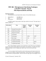
Fig. 11. Different views of Smith-Waterman irregular application
happen on this scenario. We tested the behavior of square matrixes of order 10, 25, 50, 100 and
200. Each cell of a 10
×10 matrix needs to communicate 500 Kbytes and each process occupies
1.2 Mbyte in memory (700 Kbytes comprise other application data). The cell of 25
×25 matrix
communicates 200 Kbytes and each process occupies 900 Kbytes in memory and so on.
5.2.2 Results and Discussions
Table 7 presents the application evaluation. Nineteen supersteps were crossed when a 10×10
matrix was tested. Adopting this size of matrix and α 2, 13.34s and 14.15s were obtained for
scenarios i and ii which represents a cost of 8%. The higher is the value of α, the lower is
the MigBSP overhead on application execution. This occurs because the system is stable (pro-
cesses are balanced) and α always increases at each rescheduling call. Three calls for process
relocation were done when testing α 2 (at supersteps 2, 6 and 14). The rescheduling call at
superstep 2 does not produce migrations. At this step, the load computational density is not
enough to overlap the consider migration costs involved on process transferring operation.
The same occurred on the next call at superstep 6. The last call happened at superstep 14,
which resulted on 6 migrations: {(p5,a1), (p6,a2), (p7,a3), (p8,a4), (p9,a5), (p10,a6)}. MigBSP
indicated the migration of processes that are responsible to compute the final supersteps. The
execution with α equal to 4 implies in a shorter overhead since two calls were done (at super-
steps 4 and 12). Observing scenario iii, we do not have migrations in the first call, but eight
occurred in the other one. Processes 3 up to 10 migrated in this last call to cluster Aquario. α 4
outperforms α 2 for two reasons: (i) it does less rescheduling calls and; (ii) the call that causes
process migration was done at a specific superstep in which MigBSP takes better decisions.
The system stays stable when the 25
×25 matrix was tested. α 2 produces a gain of 11% in
performance when considering 25
×25 matrix and scenario iii. This configuration presents
four calls for process rescheduling, where two of them produce migrations. No migrations
are indicated at supersteps 2 and 6. Nevertheless, processes 1 up to 12 are migrated at su-
perstep 14 while processes 21 up to 25 are transferred at superstep 30. These transferring
operations occurred to the fastest cluster. In this last call, the remaining execution presents
19 supersteps (from 31 to 49) to amortize the migration costs and to get better performance.
The execution when considering α 8 and scenario iii brings an overhead if compared with
scenario i. Two calls for migrations were done, at supersteps 8 and 24. The first call causes
Scenarios Order of considered matrices
10
×10 25×25 50×50 100×100 200×200
Scenario i 13.34s 40.74s 92.59s 162.66s 389.91s
Scenario ii
α = 2 14.15s 43.05s 95.70s 166.57s 394.68s
α = 4 14.71s 42.24s 94.84s 165.66s 393.75s
α = 8 13.78s 41.63s 94.03s 164.80s 392.85s
α = 16 13.42s 41.28s 93.36s 164.04s 392.01s
Scenario iii
α = 2 13.09s 35.97s 85.95s 150.57 374.62s
α = 4 11.94s 34.82s 84.65s 148.89s 375.53s
α = 8 13.82s 41.64s 83.00s 146.55s 374.38s
α = 16 12.40s 40.64s 85.21s 162.49s 374.40s
Table 7. Evaluation of scenarios i, ii and iii when varying the matrix size
the migration of just one process (number 1) to a1 and the second one produces three migra-
tions: {(p21,a2),(p22,a3),(p23,a4)}. We observed that processes p24 and p25 stayed on cluster
Corisco. Despite performed migrations, these two processes compromise the supersteps that
include them. Both are executing on a slower cluster and the barrier waits for the slowest pro-
cess. Maintaining the matrix size and adopting α 16, we have two calls: at supersteps 16 and
48. This last call migrates p24 an p25 to cluster Aquario. Although this movement is pertinent
to get performance, just one superstep is executed before ending the application.
Fifty processes were evaluated when the 50
×50 matrix was considered. In this context, α also
increases at each call for process rescheduling. We observed that an overhead of 3% was found
when scenario i and ii were compared (using α 2). In addition, we observed that all values of
α achieved a gain of performance in scenario iii. Especially when α 2 was used, five calls for
process rescheduling were done (at supersteps 2, 6, 14, 30 and 62). No migrations are indicated
in the first three calls. The greater is the matrix size, the greater is the amount of supersteps
needed to make migrations viable. This happens because our total load is fixed (independent
of the matrix size) but the load partition increases uniformly along the supersteps (see Section
4 for details). Process 21 up to 29 are migrated to cluster Aquario at superstep 30, while
process 37 up to 42 are migrated to this cluster at superstep 62. Using α equal to 4, 84.65s were
obtained for scenario iii which results a gain of 9%. This gain is greater than that achieved
with α 2 because now the last rescheduling call is done at superstep 60. The same processes
were migrated at this point. However, there are two more supersteps to execute using α equal
to 4. Three rescheduling calls were done with α8 (at supersteps 8, 24 and 56). Only the last two
produce migration. Three processes are migrated at superstep 24: {(p21,a1),(p22,a2),(p23,a3)}.
Process 37 up to 42 are migrated to cluster Aquario at superstep 56. This last call is efficient
since it transfers all processes from cluster Frontal to Aquario.
The execution with a 100
×100 matrix shows good results with process migration. Six
rescheduling calls were done when using α 2. Migrations did not occur at the first three su-
persteps (2, 6 and 14). Process 21 up to 29 are migrated to cluster Aquario after superstep 30.
In addition, process 37 to 42 are migrated to cluster Aquario at superstep 62. Finally, super-
step 126 indicates 7 migrations, but just 5 occurred: p30 up to p36 to cluster Aquario. These
migrations complete one process per node on cluster Aquario. MigBSP selected for migration
those processes that belonged to cluster Corisco and Frontal, which are the slowest clusters on
our infrastructure testbed. α equal to 16 produced 3 attempts for migration when a 100
×100
matrix is evaluated (at supersteps 16, 48 and 112). All of them triggered migrations. In the first
Process rescheduling: enabling performance
by applying multiple metrics and efcient adaptations 57
Fig. 11. Different views of Smith-Waterman irregular application
happen on this scenario. We tested the behavior of square matrixes of order 10, 25, 50, 100 and
200. Each cell of a 10
×10 matrix needs to communicate 500 Kbytes and each process occupies
1.2 Mbyte in memory (700 Kbytes comprise other application data). The cell of 25
×25 matrix
communicates 200 Kbytes and each process occupies 900 Kbytes in memory and so on.
5.2.2 Results and Discussions
Table 7 presents the application evaluation. Nineteen supersteps were crossed when a 10×10
matrix was tested. Adopting this size of matrix and α 2, 13.34s and 14.15s were obtained for
scenarios i and ii which represents a cost of 8%. The higher is the value of α, the lower is
the MigBSP overhead on application execution. This occurs because the system is stable (pro-
cesses are balanced) and α always increases at each rescheduling call. Three calls for process
relocation were done when testing α 2 (at supersteps 2, 6 and 14). The rescheduling call at
superstep 2 does not produce migrations. At this step, the load computational density is not
enough to overlap the consider migration costs involved on process transferring operation.
The same occurred on the next call at superstep 6. The last call happened at superstep 14,
which resulted on 6 migrations: {(p5,a1), (p6,a2), (p7,a3), (p8,a4), (p9,a5), (p10,a6)}. MigBSP
indicated the migration of processes that are responsible to compute the final supersteps. The
execution with α equal to 4 implies in a shorter overhead since two calls were done (at super-
steps 4 and 12). Observing scenario iii, we do not have migrations in the first call, but eight
occurred in the other one. Processes 3 up to 10 migrated in this last call to cluster Aquario. α 4
outperforms α 2 for two reasons: (i) it does less rescheduling calls and; (ii) the call that causes
process migration was done at a specific superstep in which MigBSP takes better decisions.
The system stays stable when the 25
×25 matrix was tested. α 2 produces a gain of 11% in
performance when considering 25
×25 matrix and scenario iii. This configuration presents
four calls for process rescheduling, where two of them produce migrations. No migrations
are indicated at supersteps 2 and 6. Nevertheless, processes 1 up to 12 are migrated at su-
perstep 14 while processes 21 up to 25 are transferred at superstep 30. These transferring
operations occurred to the fastest cluster. In this last call, the remaining execution presents
19 supersteps (from 31 to 49) to amortize the migration costs and to get better performance.
The execution when considering α 8 and scenario iii brings an overhead if compared with
scenario i. Two calls for migrations were done, at supersteps 8 and 24. The first call causes
Scenarios Order of considered matrices
10×10 25×25 50×50 100×100 200×200
Scenario i 13.34s 40.74s 92.59s 162.66s 389.91s
Scenario ii
α = 2 14.15s 43.05s 95.70s 166.57s 394.68s
α = 4 14.71s 42.24s 94.84s 165.66s 393.75s
α = 8 13.78s 41.63s 94.03s 164.80s 392.85s
α = 16 13.42s 41.28s 93.36s 164.04s 392.01s
Scenario iii
α = 2 13.09s 35.97s 85.95s 150.57 374.62s
α = 4 11.94s 34.82s 84.65s 148.89s 375.53s
α = 8 13.82s 41.64s 83.00s 146.55s 374.38s
α = 16 12.40s 40.64s 85.21s 162.49s 374.40s
Table 7. Evaluation of scenarios i, ii and iii when varying the matrix size
the migration of just one process (number 1) to a1 and the second one produces three migra-
tions: {(p21,a2),(p22,a3),(p23,a4)}. We observed that processes p24 and p25 stayed on cluster
Corisco. Despite performed migrations, these two processes compromise the supersteps that
include them. Both are executing on a slower cluster and the barrier waits for the slowest pro-
cess. Maintaining the matrix size and adopting α 16, we have two calls: at supersteps 16 and
48. This last call migrates p24 an p25 to cluster Aquario. Although this movement is pertinent
to get performance, just one superstep is executed before ending the application.
Fifty processes were evaluated when the 50
×50 matrix was considered. In this context, α also
increases at each call for process rescheduling. We observed that an overhead of 3% was found
when scenario i and ii were compared (using α 2). In addition, we observed that all values of
α achieved a gain of performance in scenario iii. Especially when α 2 was used, five calls for
process rescheduling were done (at supersteps 2, 6, 14, 30 and 62). No migrations are indicated
in the first three calls. The greater is the matrix size, the greater is the amount of supersteps
needed to make migrations viable. This happens because our total load is fixed (independent
of the matrix size) but the load partition increases uniformly along the supersteps (see Section
4 for details). Process 21 up to 29 are migrated to cluster Aquario at superstep 30, while
process 37 up to 42 are migrated to this cluster at superstep 62. Using α equal to 4, 84.65s were
obtained for scenario iii which results a gain of 9%. This gain is greater than that achieved
with α 2 because now the last rescheduling call is done at superstep 60. The same processes
were migrated at this point. However, there are two more supersteps to execute using α equal
to 4. Three rescheduling calls were done with α8 (at supersteps 8, 24 and 56). Only the last two
produce migration. Three processes are migrated at superstep 24: {(p21,a1),(p22,a2),(p23,a3)}.
Process 37 up to 42 are migrated to cluster Aquario at superstep 56. This last call is efficient
since it transfers all processes from cluster Frontal to Aquario.
The execution with a 100
×100 matrix shows good results with process migration. Six
rescheduling calls were done when using α 2. Migrations did not occur at the first three su-
persteps (2, 6 and 14). Process 21 up to 29 are migrated to cluster Aquario after superstep 30.
In addition, process 37 to 42 are migrated to cluster Aquario at superstep 62. Finally, super-
step 126 indicates 7 migrations, but just 5 occurred: p30 up to p36 to cluster Aquario. These
migrations complete one process per node on cluster Aquario. MigBSP selected for migration
those processes that belonged to cluster Corisco and Frontal, which are the slowest clusters on
our infrastructure testbed. α equal to 16 produced 3 attempts for migration when a 100
×100
matrix is evaluated (at supersteps 16, 48 and 112). All of them triggered migrations. In the first
Future Manufacturing Systems58
call, the 11
th
first processes are migrated to cluster Aquario. All process from cluster Frontal
are migrated to Aquario at superstep 48. Finally, 15 processes are selected as candidates for
migration after crossing 112 supersteps. They are: p21 to p36. This spectrum of candidates
is equal to the processes that are running on Frontal. Considering this, only 3 processes were
migrated actually: {(p34,a18),(p35a19),(p36,a20)}.
Fig. 12. Migration behavior when testing a 200 × 200 matrix with initial α equal to 2
Table 7 also shows the application performance when the 200
×200 matrix was tested. Sat-
isfactory results were obtained with process migration. The system stays stable during all
application execution. Despite having more than one process mapped to one processor, some-
times just a portion of them is responsible for computation at a specific moment. This occurs
because the processes are mapped to matrix columns, while supersteps comprise the anti-
diagonals of the matrix. Figure 12 illustrates the migrations behavior along the execution
with α 2. Using α 2 and considering scenario iii, 8 calls for process rescheduling were done.
Migrations were not done at supersteps 2, 6 and 14. Processes 21 up to 31 are migrated to
cluster Aquario at superstep 30. Moreover, all processes from cluster Frontal are migrated to
Aquario at superstep 62. Six processes are candidates for migration at superstep 126: p30 to
p36. However, only p31 up to p36 are migrated to cluster Aquario. These migrations hap-
pen because the processes initially mapped to cluster Aquario do not collaborate yet with BSP
computation. Migrations are not viable at superstep 254. Finally, 12 processes (p189 to p200)
are migrated to cluster Aquario when superstep 388 was crossed. At this time, all previous
processes allocated to Aquario are inactive and the migrations are viable. However, just 10
remaining supersteps are executed to amortize the process migration costs.
5.3 LU Decomposition Application
Consider a system of linear equations A.x = b, where A is a given n × n non singular matrix,
b a given vector of length n, and x the unknown solution vector of length n. One method for
solving this system is by using the LU Decomposition technique. It comprises the decompo-
sition of the matrix A into a lower triangular matrix L and an upper triangular matrix U such
that A = L U. A n × n matrix L is called unit lower triangular if l
i,i
= 1 for all i, 0 ≤ i < n, and
l
i,j
= 0 for all i, j where 0 ≤ i < j < n. An n × n matrix U is called upper triangular if u
i,j
= 0
for all i, j with 0
≤ j < i < n.
Fig. 13. L and U matrices with the same memory space of the original matrix A
0
1. for k from 0 to n − 1 do for k from 0 to n − 1 do
2. for j from k to n
− 1 do for i from k + 1 to n − 1 do
3. u
k,j
= a
k
k,j
a
i,k
=
a
i,k
a
k,k
4. endfor endfor
5. for i from k
+ 1 to n − 1 do for i from k + 1 to n − 1 do
6 l
k
i,k
=
a
k
i,k
u
k,k
for j from k + 1 to n − 1 do
7. endfor a
i,j
= a
i,j
− a
i,k
. a
k,j
8. for i from k + 1 to n − 1 do endfor
9. for j from k
+ 1 to n − 1 do endfor
10. a
k+1
i,j
= a
k
i,j
− l
i,k
. u
k,j
endfor
11. endfor
12. endfor
13. endfor
Fig. 14. Two algorithms to solve the LU Decomposition problem
On input, A contains the original matrix A
0
, whereas on output it contains the values of L
below the diagonal and the values of U above and on the diagonal such that LU
= A
0
. Figure
13 illustrates the organization of LU computation. The values of L and U computed so far
and the computed sub-matrix A
k
may be stored in the same memory space of A
0
. Figure 14
presents the sequential algorithm for producing L and U in stages. Stage k first computes the
elements u
k,j
, j ≥ k, of row k of U and the elements l
i,k
, i > k, of column k of L. Then, it
computes A
k+1
in preparation for the next stage. Figure 14 also presents in the right side the
functioning of the previous algorithm using just the elements from matrix A. Figure 13 (b)
presents the data that is necessary to compute a
i,j
. Besides its own value, a
i,j
is updated using
a value from the same line and another from the same column.
5.3.1 Modeling the Problem
This section explains how we modeled the LU sequential application on a BSP-based parallel
one. Firstly, the bulk of the computational work in stage k of the sequential algorithm is the
Process rescheduling: enabling performance
by applying multiple metrics and efcient adaptations 59
call, the 11
th
first processes are migrated to cluster Aquario. All process from cluster Frontal
are migrated to Aquario at superstep 48. Finally, 15 processes are selected as candidates for
migration after crossing 112 supersteps. They are: p21 to p36. This spectrum of candidates
is equal to the processes that are running on Frontal. Considering this, only 3 processes were
migrated actually: {(p34,a18),(p35a19),(p36,a20)}.
Fig. 12. Migration behavior when testing a 200 × 200 matrix with initial α equal to 2
Table 7 also shows the application performance when the 200
×200 matrix was tested. Sat-
isfactory results were obtained with process migration. The system stays stable during all
application execution. Despite having more than one process mapped to one processor, some-
times just a portion of them is responsible for computation at a specific moment. This occurs
because the processes are mapped to matrix columns, while supersteps comprise the anti-
diagonals of the matrix. Figure 12 illustrates the migrations behavior along the execution
with α 2. Using α 2 and considering scenario iii, 8 calls for process rescheduling were done.
Migrations were not done at supersteps 2, 6 and 14. Processes 21 up to 31 are migrated to
cluster Aquario at superstep 30. Moreover, all processes from cluster Frontal are migrated to
Aquario at superstep 62. Six processes are candidates for migration at superstep 126: p30 to
p36. However, only p31 up to p36 are migrated to cluster Aquario. These migrations hap-
pen because the processes initially mapped to cluster Aquario do not collaborate yet with BSP
computation. Migrations are not viable at superstep 254. Finally, 12 processes (p189 to p200)
are migrated to cluster Aquario when superstep 388 was crossed. At this time, all previous
processes allocated to Aquario are inactive and the migrations are viable. However, just 10
remaining supersteps are executed to amortize the process migration costs.
5.3 LU Decomposition Application
Consider a system of linear equations A.x = b, where A is a given n × n non singular matrix,
b a given vector of length n, and x the unknown solution vector of length n. One method for
solving this system is by using the LU Decomposition technique. It comprises the decompo-
sition of the matrix A into a lower triangular matrix L and an upper triangular matrix U such
that A = L U. A n × n matrix L is called unit lower triangular if l
i,i
= 1 for all i, 0 ≤ i < n, and
l
i,j
= 0 for all i, j where 0 ≤ i < j < n. An n × n matrix U is called upper triangular if u
i,j
= 0
for all i, j with 0
≤ j < i < n.
Fig. 13. L and U matrices with the same memory space of the original matrix A
0
1. for k from 0 to n − 1 do for k from 0 to n − 1 do
2. for j from k to n
− 1 do for i from k + 1 to n − 1 do
3. u
k,j
= a
k
k,j
a
i,k
=
a
i,k
a
k,k
4. endfor endfor
5. for i from k
+ 1 to n − 1 do for i from k + 1 to n − 1 do
6 l
k
i,k
=
a
k
i,k
u
k,k
for j from k + 1 to n − 1 do
7. endfor a
i,j
= a
i,j
− a
i,k
. a
k,j
8. for i from k + 1 to n − 1 do endfor
9. for j from k
+ 1 to n − 1 do endfor
10. a
k+1
i,j
= a
k
i,j
− l
i,k
. u
k,j
endfor
11. endfor
12. endfor
13. endfor
Fig. 14. Two algorithms to solve the LU Decomposition problem
On input, A contains the original matrix A
0
, whereas on output it contains the values of L
below the diagonal and the values of U above and on the diagonal such that LU
= A
0
. Figure
13 illustrates the organization of LU computation. The values of L and U computed so far
and the computed sub-matrix A
k
may be stored in the same memory space of A
0
. Figure 14
presents the sequential algorithm for producing L and U in stages. Stage k first computes the
elements u
k,j
, j ≥ k, of row k of U and the elements l
i,k
, i > k, of column k of L. Then, it
computes A
k+1
in preparation for the next stage. Figure 14 also presents in the right side the
functioning of the previous algorithm using just the elements from matrix A. Figure 13 (b)
presents the data that is necessary to compute a
i,j
. Besides its own value, a
i,j
is updated using
a value from the same line and another from the same column.
5.3.1 Modeling the Problem
This section explains how we modeled the LU sequential application on a BSP-based parallel
one. Firstly, the bulk of the computational work in stage k of the sequential algorithm is the
Future Manufacturing Systems60
modification of the matrix elements a
i,j
with i, j ≥ k + 1. Aiming to prevent communication
of large amounts of data, the update of a
i,j
= a
i,j
+ a
i,k
.a
k,j
must be performed by the process
whose contains a
i,j
. This implies that only elements of column k and row k of A need to be
communicated in stage k in order to compute the new sub-matrix A
k
. An important obser-
vation is that the modification of the elements in row A
(i, k + 1 : n − 1) uses only one value
of column k of A, namely a
i,k
. The provided notation A(i, k + 1 : n − 1) denotes the cells of
line i varying from column k
+ 1 to n − 1. If we distribute each matrix row over a limit set
of N processes, then the communication of an element from column k can be restricted to a
multicast to N processes. Similarly, the change of the elements in A
(k + 1 : n − 1, j) uses only
one value from row k of A, namely a
k,j
. If we divide each column over a set of M processes,
the communication of an element of row k can be restricted to a multicast to M processes.
We are using a Cartesian scheme for the distribution of matrices. The square cyclic distribution
is used since it is particularly suitable for matrix computations (Bisseling, 2004). Thus, it is
natural to organize the processes by two-dimensional identifiers P
(s, t) with 0 ≤ s < M and
0
≤ t < N, where the number of processes p = M.N. Figure 15 depicts a 6 × 6 matrix mapped
to 6 processes, where M
= 2 and N = 3. Assuming that M and N are factors of n, each process
will store nc (number of cells) cells in memory (see Equation 10).
nc
=
n
M
.
n
N
(10)
Fig. 15. Cartesian distribution of a matrix over 2×3 (M × N) processes
A parallel algorithm uses data parallelism for computations and the need-to-know principle
to design the communication phase of each superstep. Following the concepts of BSP, all
communication performed during a superstep will be completed when finishing it and the
data will be available at the beginning of the next superstep (Bonorden, 2007). Concerning
this, we modeled our algorithm using three kinds of supersteps. They are explained in Table
8. The element a
k,k
is passed to the process that computes a
i,k
in the first kind of superstep.
The computation of a
i,k
is expressed in the beginning of the second superstep. This superstep
is also responsible for sending the elements a
i,k
and a
k,j
to a
i,j
. First of all, we pass the element
a
i,k
, k + 1 ≤ i < n, to the N − 1 processes that execute on the respective row i. This kind of
superstep also comprises the passing of a
k,j
, k + 1 ≤ j < n, to M − 1 processes which execute
on the respective column j. The superstep 3 considers the computation of a
i,j
, the increase of
k (next stage of the algorithm) and the transmission of a
k,k
to a
i,k
elements (k + 1 ≤ i < n).
The application will execute one superstep of type 1 and will follow with the interleaving of
supersteps 2 and 3. Thus, a n
× n matrix will trigger 2n + 1 supersteps in our LU modeling. We
Type of su-
perstep
Steps and explanation
First
Step 1.1 : k = 0
Step 1.2 - Pass the element a
k,k
to cells which will compute a
i,k
(k + 1 ≤ i <
n)
Second
Step 2.1 : Computation of a
i,k
(k + 1 ≤ i < n) by cells which own them
Step 2.2 : For each i (k
+ 1 ≤ i < n), pass the element a
i,k
to other a
i,j
elements in the same line (k + 1 ≤ j < n)
Step 2.3 : For each j (k
+ 1 ≤ j < n), pass the element a
k,j
to other a
i,j
elements in the same column (k + 1 ≤ i < n)
Third
Step 3.1 : For each i and j (k
+ 1 ≤ i, j < n), calculate a
i,j
as a
i,j
+ a
i,k
.a
k,j
Step 3.2 : k = k + 1
Step 3.3 : Pass the element a
k,k
to cells which will compute a
i,k
(k + 1 ≤ i <
n)
Table 8. Modeling three types of supersteps for LU computation
modeled the Cartesian distribution M
× N in the following manner: 5 × 5, 10 × 5, 10 × 10 and
20
× 10 for 25, 50, 100 and 200 processes, respectively. Moreover, we are applying simulation
over square matrices with orders 500, 1000, 2000 and 5000. Lastly, the tests were executed
using α
= 4, ω = 3, D = 0.5 and x = 80%.
5.3.2 Results and Discussions
Table 9 presents the results when evaluating LU application. The tests with the first matrix
size show the worst results. Formerly, the higher the number of processes, the worse the
performance, as we can observe in scenario i. The reasons for the observed times are the
overheads related to communication and synchronization. Secondly, MigBSP indicated that
all migration attempts were not viable due to low computing and communication loads when
compared to migration costs. Considering this, both scenarios ii and iii have the same results.
Processes
500
×500 matrix 1000×1000 matrix 2000×2000 matrix
i ii iii i ii iii i ii iii
25 1.68 2.42 2.42 11.65 13.13 10.24 90.11 91.26 76.20
50 2.59 3.54 3.34 10.10 11.18 9.63 60.23 61.98 54.18
100 6.70 7.81 7.65 15.22 16.21 16.21 48.79 50.25 46.87
200 13.23 14.89 14.89 28.21 30.46 30.46 74.14 76.97 76.97
Table 9. First results when executing LU linked to MigBSP (time in seconds)
When testing a 1000
× 1000 matrix with 25 processes, the first rescheduling call does not cause
migrations. After this call at superstep 4, the next one at superstep 11 informs the migration of
5 processes from cluster Corisco. They were all transferred to cluster Aquario, which has the
highest computation power. MigBSP does not point migrations in the future calls. α always
increases its value at each rescheduling call since the processes are balanced after the men-
tioned relocations. MigBSP obtained a gain of 12% of performance with 25 processes when
comparing scenarios i and iii. With the same size of matrix and 50 processes, 6 processes from
Frontal were migrated to Aquario at superstep 9. Although these migrations are profitable,
Process rescheduling: enabling performance
by applying multiple metrics and efcient adaptations 61
modification of the matrix elements a
i,j
with i, j ≥ k + 1. Aiming to prevent communication
of large amounts of data, the update of a
i,j
= a
i,j
+ a
i,k
.a
k,j
must be performed by the process
whose contains a
i,j
. This implies that only elements of column k and row k of A need to be
communicated in stage k in order to compute the new sub-matrix A
k
. An important obser-
vation is that the modification of the elements in row A
(i, k + 1 : n − 1) uses only one value
of column k of A, namely a
i,k
. The provided notation A(i, k + 1 : n − 1) denotes the cells of
line i varying from column k
+ 1 to n − 1. If we distribute each matrix row over a limit set
of N processes, then the communication of an element from column k can be restricted to a
multicast to N processes. Similarly, the change of the elements in A
(k + 1 : n − 1, j) uses only
one value from row k of A, namely a
k,j
. If we divide each column over a set of M processes,
the communication of an element of row k can be restricted to a multicast to M processes.
We are using a Cartesian scheme for the distribution of matrices. The square cyclic distribution
is used since it is particularly suitable for matrix computations (Bisseling, 2004). Thus, it is
natural to organize the processes by two-dimensional identifiers P
(s, t) with 0 ≤ s < M and
0
≤ t < N, where the number of processes p = M.N. Figure 15 depicts a 6 × 6 matrix mapped
to 6 processes, where M
= 2 and N = 3. Assuming that M and N are factors of n, each process
will store nc (number of cells) cells in memory (see Equation 10).
nc
=
n
M
.
n
N
(10)
Fig. 15. Cartesian distribution of a matrix over 2×3 (M × N) processes
A parallel algorithm uses data parallelism for computations and the need-to-know principle
to design the communication phase of each superstep. Following the concepts of BSP, all
communication performed during a superstep will be completed when finishing it and the
data will be available at the beginning of the next superstep (Bonorden, 2007). Concerning
this, we modeled our algorithm using three kinds of supersteps. They are explained in Table
8. The element a
k,k
is passed to the process that computes a
i,k
in the first kind of superstep.
The computation of a
i,k
is expressed in the beginning of the second superstep. This superstep
is also responsible for sending the elements a
i,k
and a
k,j
to a
i,j
. First of all, we pass the element
a
i,k
, k + 1 ≤ i < n, to the N − 1 processes that execute on the respective row i. This kind of
superstep also comprises the passing of a
k,j
, k + 1 ≤ j < n, to M − 1 processes which execute
on the respective column j. The superstep 3 considers the computation of a
i,j
, the increase of
k (next stage of the algorithm) and the transmission of a
k,k
to a
i,k
elements (k + 1 ≤ i < n).
The application will execute one superstep of type 1 and will follow with the interleaving of
supersteps 2 and 3. Thus, a n
× n matrix will trigger 2n + 1 supersteps in our LU modeling. We
Type of su-
perstep
Steps and explanation
First
Step 1.1 : k = 0
Step 1.2 - Pass the element a
k,k
to cells which will compute a
i,k
(k + 1 ≤ i <
n)
Second
Step 2.1 : Computation of a
i,k
(k + 1 ≤ i < n) by cells which own them
Step 2.2 : For each i (k + 1 ≤ i < n), pass the element a
i,k
to other a
i,j
elements in the same line (k + 1 ≤ j < n)
Step 2.3 : For each j (k + 1 ≤ j < n), pass the element a
k,j
to other a
i,j
elements in the same column (k + 1 ≤ i < n)
Third
Step 3.1 : For each i and j (k + 1 ≤ i, j < n), calculate a
i,j
as a
i,j
+ a
i,k
.a
k,j
Step 3.2 : k = k + 1
Step 3.3 : Pass the element a
k,k
to cells which will compute a
i,k
(k + 1 ≤ i <
n)
Table 8. Modeling three types of supersteps for LU computation
modeled the Cartesian distribution M
× N in the following manner: 5 × 5, 10 × 5, 10 × 10 and
20
× 10 for 25, 50, 100 and 200 processes, respectively. Moreover, we are applying simulation
over square matrices with orders 500, 1000, 2000 and 5000. Lastly, the tests were executed
using α
= 4, ω = 3, D = 0.5 and x = 80%.
5.3.2 Results and Discussions
Table 9 presents the results when evaluating LU application. The tests with the first matrix
size show the worst results. Formerly, the higher the number of processes, the worse the
performance, as we can observe in scenario i. The reasons for the observed times are the
overheads related to communication and synchronization. Secondly, MigBSP indicated that
all migration attempts were not viable due to low computing and communication loads when
compared to migration costs. Considering this, both scenarios ii and iii have the same results.
Processes
500×500 matrix 1000×1000 matrix 2000×2000 matrix
i ii iii i ii iii i ii iii
25 1.68 2.42 2.42 11.65 13.13 10.24 90.11 91.26 76.20
50 2.59 3.54 3.34 10.10 11.18 9.63 60.23 61.98 54.18
100 6.70 7.81 7.65 15.22 16.21 16.21 48.79 50.25 46.87
200 13.23 14.89 14.89 28.21 30.46 30.46 74.14 76.97 76.97
Table 9. First results when executing LU linked to MigBSP (time in seconds)
When testing a 1000
× 1000 matrix with 25 processes, the first rescheduling call does not cause
migrations. After this call at superstep 4, the next one at superstep 11 informs the migration of
5 processes from cluster Corisco. They were all transferred to cluster Aquario, which has the
highest computation power. MigBSP does not point migrations in the future calls. α always
increases its value at each rescheduling call since the processes are balanced after the men-
tioned relocations. MigBSP obtained a gain of 12% of performance with 25 processes when
comparing scenarios i and iii. With the same size of matrix and 50 processes, 6 processes from
Frontal were migrated to Aquario at superstep 9. Although these migrations are profitable,
Future Manufacturing Systems62
they do not provide stability to the system and the processes remain unbalanced among the
resources. Migrations are not viable in the next 3 calls at supersteps 15, 21 and 27. After
that, MigBSP launches our second adaptation on rescheduling frequency in order to alleviate
its impact and α begins to grow until the end of the application. The tests with 50 processes
obtained gains of just 5% with process migration. This is explained by the fact that the compu-
tational load is decreased in this configuration when compared to the one with 25 processes.
In addition, the bigger the number of the superstep, the smaller the computational load re-
quired by it. Therefore, the more advanced the execution, the lesser the gain with migrations.
The tests with 100 and 200 processes do not present migrations owing to the forces that act in
favor of migration are weaker than the Memory metric in all rescheduling calls.
The execution with a 2000
× 2000 matrix presents good results because the computational load
is increased. We observed a gain of 15% with process relocation when testing 25 processes.
All processes from cluster Corisco were migrated to Aquario in the first rescheduling call (at
superstep 4). Thus, the application can take profit from this relocation in its beginning, when
it demands more computations. The time for concluding the LU application is reduced when
passing from 25 to 50 processes as we can see in scenario i. However, the use of MigBSP
resulted in lower gains. Scenario i presented 60.23s while scenario iii achieved 56.18s (9% of
profit). When considering 50 processes, 6 processes were transferred from cluster Frontal to
Aquario at superstep 4. The next call occurs at superstep 9, where 16 processes from cluster
Corisco were elected as migration candidates to Aquario. However, MigBSP indicated the
migration of 14 processes, since there were only 14 unoccupied processors in the target cluster.
Fig. 16. Performance graph with our three scenarios for a 5000 × 5000 matrix
We observed that the higher the matrix order, the better the results with process migration.
Considering this, the evaluation of a 5000
× 5000 matrix can be seen in the Figure 16. The sim-
ple movement of all processes from cluster Corisco to Aquario represented a gain of 19% when
executing 25 processes. The tests with 50 processes obtained 852.31s and 723.64s for scenario
i and iii, respectively. The same migration behavior found on the tests with the 2000
× 2000
matrix was achieved in Scenario iii However, the increase of matrix order represented a gain
of 15% (order 5000) instead of 10% (order 2000). This analysis helps us to verify our previ-
ous hypothesis about performance gains when enlarging the matrix. Finally, the tests with
200 processes indicated the migration of 6 processes (p195 up to p200) from cluster Corisco to
Aquario at superstep 4. Thus, the nodes that belong to Corisco just execute one BSP process
while the nodes from Aquario begin to treat 2 processes. The remaining rescheduling calls
inform the processes from Labtec as those with the higher values of PM. However, their mi-
grations are not considered profitable. The final execution with 200 processes achieved 460.85s
and 450.33s for scenarios i and iii, respectively.
6. Conclusion
Scheduling schemes for multi-programmed parallel systems can be viewed in two lev-
els (Frachtenberg & Schwiegelshohn, 2008). In the first level processors are allocated to a
job. In the second level processes from a job are (re)scheduled using this pool of processors.
MigBSP can be included in this last scheme, offering algorithms for load (BSP processes) re-
balancing among the resources during the application runtime. In the best of our knowledge,
MigBSP is the pioneer model on treating BSP process rescheduling with three metrics and
adaptations on remapping frequency. These features are enabled by MigBSP at middleware
level, without changing the application code.
Considering the spectrum of the three tested applications, we can take the following conclu-
sions in a nutshell: (i) the larger the computing grain, the better the gain with processes migra-
tion; (ii) MigBSP does not indicate the migration of those processes that have high migration
costs when compared to computation and communication loads; (iii) MigBSP presented a low
overhead on application execution when migrations are not applied; (v) our tests prioritizes
migrations to cluster Aquario since it is the fastest one among considered clusters and tested
applications are CPU-bound and; (vi) MigBSP does not work with previous knowledge about
application. Considering this last topic, MigBSP indicates migrations even when the applica-
tion is close to finish. In this situation, these migrations bring an overhead since the remaining
time for application conclusion is too short to amortize their costs.
The results showed that MigBSP presented a low overhead on application execution. The
calculus of the PM (Potential of Migration) as well as our efficient adaptations were respon-
sible for this feature. PM considers processes and Sets (different sites), not performing all
processes-resources tests at the rescheduling moment. Meanwhile, our adaptations were cru-
cial to enable MigBSP as a viable scheduler. Instead of performing the rescheduling call at
each fixed interval, they manage a flexible interval between calls based on the behavior of the
processes. The concepts of the adaptations are: (i) to postpone the rescheduling call if the
system is stable (processes are balanced) or to turn it more frequent, otherwise; (ii) to delay
this call if a pattern without migrations in ω calls is observed.
7. References
Bhandarkar, M. A., Brunner, R. & Kale, L. V. (2000). Run-time support for adaptive load
balancing, IPDPS ’00: Proceedings of the 15 IPDPS 2000 Workshops on Parallel and Dis-
tributed Processing, Springer-Verlag, London, UK, pp. 1152–1159.
Bisseling, R. H. (2004). Parallel Scientific Computation: A Structured Approach Using BSP and
MPI, Oxford University Press.
Bonorden, O. (2007). Load balancing in the bulk-synchronous-parallel setting using process
migrations., 21th International Parallel and Distributed Processing Symposium (IPDPS
2007), IEEE, pp. 1–9.
Bonorden, O., Gehweiler, J. & auf der Heide, F. M. (2005). Load balancing strategies in a web
computing environment, Proceeedings of International Conference on Parallel Processing
and Applied Mathematics (PPAM), Poznan, Poland, pp. 839–846.
Casanova, H., Legrand, A. & Quinson, M. (2008). Simgrid: A generic framework for large-
scale distributed experiments, Tenth International Conference on Computer Modeling and
Simulation (uksim), IEEE Computer Society, Los Alamitos, CA, USA, pp. 126–131.
Casavant, T. L. & Kuhl, J. G. (1988). A taxonomy of scheduling in general-purpose distributed
computing systems, IEEE Trans. Softw. Eng. 14(2): 141–154.
Process rescheduling: enabling performance
by applying multiple metrics and efcient adaptations 63
they do not provide stability to the system and the processes remain unbalanced among the
resources. Migrations are not viable in the next 3 calls at supersteps 15, 21 and 27. After
that, MigBSP launches our second adaptation on rescheduling frequency in order to alleviate
its impact and α begins to grow until the end of the application. The tests with 50 processes
obtained gains of just 5% with process migration. This is explained by the fact that the compu-
tational load is decreased in this configuration when compared to the one with 25 processes.
In addition, the bigger the number of the superstep, the smaller the computational load re-
quired by it. Therefore, the more advanced the execution, the lesser the gain with migrations.
The tests with 100 and 200 processes do not present migrations owing to the forces that act in
favor of migration are weaker than the Memory metric in all rescheduling calls.
The execution with a 2000
× 2000 matrix presents good results because the computational load
is increased. We observed a gain of 15% with process relocation when testing 25 processes.
All processes from cluster Corisco were migrated to Aquario in the first rescheduling call (at
superstep 4). Thus, the application can take profit from this relocation in its beginning, when
it demands more computations. The time for concluding the LU application is reduced when
passing from 25 to 50 processes as we can see in scenario i. However, the use of MigBSP
resulted in lower gains. Scenario i presented 60.23s while scenario iii achieved 56.18s (9% of
profit). When considering 50 processes, 6 processes were transferred from cluster Frontal to
Aquario at superstep 4. The next call occurs at superstep 9, where 16 processes from cluster
Corisco were elected as migration candidates to Aquario. However, MigBSP indicated the
migration of 14 processes, since there were only 14 unoccupied processors in the target cluster.
Fig. 16. Performance graph with our three scenarios for a 5000 × 5000 matrix
We observed that the higher the matrix order, the better the results with process migration.
Considering this, the evaluation of a 5000
× 5000 matrix can be seen in the Figure 16. The sim-
ple movement of all processes from cluster Corisco to Aquario represented a gain of 19% when
executing 25 processes. The tests with 50 processes obtained 852.31s and 723.64s for scenario
i and iii, respectively. The same migration behavior found on the tests with the 2000
× 2000
matrix was achieved in Scenario iii However, the increase of matrix order represented a gain
of 15% (order 5000) instead of 10% (order 2000). This analysis helps us to verify our previ-
ous hypothesis about performance gains when enlarging the matrix. Finally, the tests with
200 processes indicated the migration of 6 processes (p195 up to p200) from cluster Corisco to
Aquario at superstep 4. Thus, the nodes that belong to Corisco just execute one BSP process
while the nodes from Aquario begin to treat 2 processes. The remaining rescheduling calls
inform the processes from Labtec as those with the higher values of PM. However, their mi-
grations are not considered profitable. The final execution with 200 processes achieved 460.85s
and 450.33s for scenarios i and iii, respectively.
6. Conclusion
Scheduling schemes for multi-programmed parallel systems can be viewed in two lev-
els (Frachtenberg & Schwiegelshohn, 2008). In the first level processors are allocated to a
job. In the second level processes from a job are (re)scheduled using this pool of processors.
MigBSP can be included in this last scheme, offering algorithms for load (BSP processes) re-
balancing among the resources during the application runtime. In the best of our knowledge,
MigBSP is the pioneer model on treating BSP process rescheduling with three metrics and
adaptations on remapping frequency. These features are enabled by MigBSP at middleware
level, without changing the application code.
Considering the spectrum of the three tested applications, we can take the following conclu-
sions in a nutshell: (i) the larger the computing grain, the better the gain with processes migra-
tion; (ii) MigBSP does not indicate the migration of those processes that have high migration
costs when compared to computation and communication loads; (iii) MigBSP presented a low
overhead on application execution when migrations are not applied; (v) our tests prioritizes
migrations to cluster Aquario since it is the fastest one among considered clusters and tested
applications are CPU-bound and; (vi) MigBSP does not work with previous knowledge about
application. Considering this last topic, MigBSP indicates migrations even when the applica-
tion is close to finish. In this situation, these migrations bring an overhead since the remaining
time for application conclusion is too short to amortize their costs.
The results showed that MigBSP presented a low overhead on application execution. The
calculus of the PM (Potential of Migration) as well as our efficient adaptations were respon-
sible for this feature. PM considers processes and Sets (different sites), not performing all
processes-resources tests at the rescheduling moment. Meanwhile, our adaptations were cru-
cial to enable MigBSP as a viable scheduler. Instead of performing the rescheduling call at
each fixed interval, they manage a flexible interval between calls based on the behavior of the
processes. The concepts of the adaptations are: (i) to postpone the rescheduling call if the
system is stable (processes are balanced) or to turn it more frequent, otherwise; (ii) to delay
this call if a pattern without migrations in ω calls is observed.
7. References
Bhandarkar, M. A., Brunner, R. & Kale, L. V. (2000). Run-time support for adaptive load
balancing, IPDPS ’00: Proceedings of the 15 IPDPS 2000 Workshops on Parallel and Dis-
tributed Processing, Springer-Verlag, London, UK, pp. 1152–1159.
Bisseling, R. H. (2004). Parallel Scientific Computation: A Structured Approach Using BSP and
MPI, Oxford University Press.
Bonorden, O. (2007). Load balancing in the bulk-synchronous-parallel setting using process
migrations., 21th International Parallel and Distributed Processing Symposium (IPDPS
2007), IEEE, pp. 1–9.
Bonorden, O., Gehweiler, J. & auf der Heide, F. M. (2005). Load balancing strategies in a web
computing environment, Proceeedings of International Conference on Parallel Processing
and Applied Mathematics (PPAM), Poznan, Poland, pp. 839–846.
Casanova, H., Legrand, A. & Quinson, M. (2008). Simgrid: A generic framework for large-
scale distributed experiments, Tenth International Conference on Computer Modeling and
Simulation (uksim), IEEE Computer Society, Los Alamitos, CA, USA, pp. 126–131.
Casavant, T. L. & Kuhl, J. G. (1988). A taxonomy of scheduling in general-purpose distributed
computing systems, IEEE Trans. Softw. Eng. 14(2): 141–154.
Future Manufacturing Systems64
Chen, L., Wang, C L. & Lau, F. (2008). Process reassignment with reduced migration cost
in grid load rebalancing, Parallel and Distributed Processing, 2008. IPDPS 2008. IEEE
International Symposium on pp. 1–13.
Du, C., Ghosh, S., Shankar, S. & Sun, X H. (2004). A runtime system for autonomic reschedul-
ing of mpi programs, ICPP ’04: Proceedings of the 2004 International Conference on Par-
allel Processing, IEEE Computer Society, Washington, DC, USA, pp. 4–11.
Du, C., Sun, X H. & Wu, M. (2007). Dynamic scheduling with process migration, CCGRID
’07: Proceedings of the Seventh IEEE International Symposium on Cluster Computing and
the Grid, IEEE Computer Society, Washington, DC, USA, pp. 92–99.
Frachtenberg, E. & Schwiegelshohn, U. (2008). New Challenges of Parallel Job Scheduling, Job
Scheduling Strategies for Parallel Processing 4942: 1–23.
Heiss, H U. & Schmitz, M. (1995). Decentralized dynamic load balancing: the particles ap-
proach, Inf. Sci. Inf. Comput. Sci. 84(1-2): 115–128.
Hernandez, I. & Cole, M. (2007). Scheduling dags on grids with copying and migration., in
R. Wyrzykowski, J. Dongarra, K. Karczewski & J. Wasniewski (eds), PPAM, Vol. 4967
of Lecture Notes in Computer Science, Springer, pp. 1019–1028.
Huang, C., Zheng, G., Kalé, L. & Kumar, S. (2006). Performance evaluation of adaptive
mpi, PPoPP ’06: Proceedings of the eleventh ACM SIGPLAN symposium on Principles and
practice of parallel programming, ACM Press, New York, NY, USA, pp. 12–21.
Kondo, D., Casanova, H., Wing, E. & Berman, F. (2002). Models and scheduling mechanisms
for global computing applications, IPDPS ’02: Proceedings of the 16th International
Symposium on Parallel and Distributed Processing, IEEE Computer Society, Washing-
ton, DC, USA, p. 79.2.
Low, M. Y H., Liu, W. & Schmidt, B. (2007). A parallel bsp algorithm for irregular dynamic
programming, Advanced Parallel Processing Technologies, 7th International Symposium,
Vol. 4847 of Lecture Notes in Computer Science, Springer, pp. 151–160.
Milanés, A., Rodriguez, N. & Schulze, B. (2008). State of the art in heterogeneous strong
migration of computations, Concurr. Comput. : Pract. Exper. 20(13): 1485–1508.
Moreno-Vozmediano, R. & Alonso-Conde, A. B. (2005). Influence of grid economic factors
on scheduling and migration., High Performance Computing for Computational Science -
VECPAR, Vol. 3402 of Lecture Notes in Computer Science, Springer, pp. 274–287.
Sánchez, A., Pérez, M. S., Montes, J. & Cortes, T. (2010). A high performance suite of data
services for grids, Future Gener. Comput. Syst. 26(4): 622–632.
Schepke, Claudio; Maillard, N. (2007). Performance improvement of the parallel lattice boltz-
mann method through blocked data distributions, 19th International Symposium on
Computer Architecture and High Performance Computing, 2007. SBAC-PAD 2007, pp. 71–
78.
Smith, J. M. (1988). A survey of process migration mechanisms, SIGOPS Oper. Syst. Rev.
22(3): 28–40.
Tanenbaum, A. (2003). Computer Networks, 4th edn, Prentice Hall PTR, Upper Saddle River,
New Jersey.
Utrera, G., Corbalan, J. & Labarta, J. (2005). Dynamic load balancing in mpi jobs, The 6th
International Symposium on High Performance Computing.
Vadhiyar, S. S. & Dongarra, J. J. (2005). Self adaptivity in grid computing: Research articles,
Concurr. Comput. : Pract. Exper. 17(2-4): 235–257.
Valiant, L. G. (1990). A bridging model for parallel computation, Commun. ACM 33(8): 103–
111.
Reliability Modeling and Analysis of Flexible Manufacturing Cells 65
Reliability Modeling and Analysis of Flexible Manufacturing Cells
Mehmet Savsar
X
Reliability modeling and analysis
of flexible manufacturing cells
Mehmet Savsar
Kuwait University
Kuwait
1. Introduction
During the past half century, market competition has been very intense and production
companies have been trying to find more efficient ways to manufacture their products.
While during the period 1960 to 1970 manufacturing cost was the primary concern, later it
was followed by product quality and delivery speed. New strategies had to be formulated
by companies to adapt to the environment in which they operate, to be more flexible in their
operations, and to satisfy different market segments. As a result of these efforts, a new
manufacturing technology, called Flexible Manufacturing Systems (FMS), was innovated.
FMS is a philosophy, in which "systems" is the key concept. A system view is incorporated
into manufacturing. FMS is also one way that manufacturers are able to achieve agility, to
have fastest response to the market, to operate with the lowest total cost, and to gain the
greatest skills in satisfying the customers.
Today flexibility means to produce reasonably priced customized products of high quality
that can be quickly delivered to customers. With respect to manufacturing, flexibility could
mean the capability of producing different products without major retooling; ability to
change an old line to produce new products; or the ability to change a production schedule
to handle multiple parts. From customer’s point of view, flexibility is the ability to have
flexible speed of delivery. With respect to operations, flexibility means the ability to
efficiently produce highly customized and unique products. With respect to capacity,
flexibility means the ability to rapidly increase or decrease production levels or to shift
capacity quickly from one product or service to another. Finally, strategically flexibility
means the ability of a company to offer a wide variety of products to its customers. In a
manufacturing system, machine flexibility, material handling flexibility, and operation
flexibility are the important aspects considered.
The idea of an FMS was proposed in England in 1960s under the name "System 24", which
was a flexible machining system that could operate without human operators 24 hours a day
under computer control. Initial emphasis was on automation rather than the reorganization
of workflow. Initial FMS were very large and complex, consisting of many Computer
Numerical Controlled (CNC) machines and sophisticated material handling systems, such
4
Future Manufacturing Systems66
as robots, automated guided vehicles (AGV) and automated pallets, all controlled by
complex software. Part and tool handling robots could handle any family of parts for which
the system had been designed and developed. Only a limited number of industries could
afford investing in a highly expensive FMS as described above. However, the current trend
is toward small versions of the traditional FMS, called flexible manufacturing cells (FMC) or
flexible manufacturing modules (FMM). Today one or more CNC machines served by one
or more robots and a pallet system are considered a flexible cell and two ore more cells are
considered as a flexible manufacturing system. Other related systems are Flexible Assembly
Cells (FAC), Flexible Manufacturing Groups (FMG), Flexible Production Systems (FPS), and
Flexible Manufacturing Lines (FML).
A basic FMC consists of a robot, one or more flexible machines including inspection, and an
external material handling system such as an automated pallet for moving blanks and
finished parts into and out of the cell. The robot is utilized for internal material handling
which includes machine loading and unloading. The FMC is capable of doing different
operations on a variety of parts, which usually form a part family with selection by a group
technology approach. Chan and Bedworth (1990) indicated that the most feasible approach
to automate a production system with flexibility is to initially incorporate small FMC into
the system. This approach requires lower investment, less risk, and also satisfies many of the
benefits gained through larger and more costly structures, such as flexible manufacturing
systems (FMS). While FMS are very expensive and generally require investments in millions
of dollars, FMC are less costly, smaller and less complex systems. Therefore, for smaller
companies with restricted capital resources, a gradual integration is initiated with limited
investment in a small FMC, which facilitates subsequent integration into a larger system,
such as an FMS.
Machining cells are widely used in industry to process a variety of parts to achieve high
productivity in production environments with rapidly changing product structures and
customer demand. They offer flexibility to be adapted to the changes in operational
requirements. There are various types of Flexible Manufacturing Cells (FMC) incorporated
into Flexible Manufacturing Systems (FMS) with a variety of flexible machines for discrete
part machining. In addition to discrete part machining systems, there are different types of
assembly machines and CNC punching press systems, which are also configured as flexible
cells. FMS and FMC performance depends on several operational and system characteristics,
which may include part scheduling and system operational characteristics. In the past, most
of the FMC related research has been in the areas of part scheduling and system control.
Scheduling algorithms are developed to determine the best processing sequence of parts to
optimize FMC performance and equipment utilization. It has also been realized that system
characteristics, such as design configuration and operation of an FMC have significant effect
on its performance. Machining rate, pallet capacity, robot and pallet speed, and equipment
failure and repair rates are important system characteristics affecting FMC performance.
Several models have been developed for FMS and FMC in relation to the effects of different
parameters on system performance. Wang and Wan (1993) studied the dynamic reliability of
a FMS based on fuzzy information. Yuanidis et al. (1994) used a heuristic procedure called
group method of data handling to asses FMS reliability with minimal data available. Han et
al. (2006) analyzed FMC reliability through the method of fuzzy fault tree based on
triangular fuzzy membership. Khodabandehloo and Sayles (2007) investigated the
applicability of fault tree analysis and event tree analysis to production reliability in FMS
and concluded that event tree analysis was more effective in solving this problem. Henneke
and Choi (1990), Savsar and Cogun (1993), and Cogun and Savsar (1996) have presented
stochastic and simulation models for evaluating the performance of FMC and FMS with
respect to system configuration and component speeds, such as machining rate, robot and
pallet speeds. Koulamas (1992) and Savsar (2000) have looked into the reliability and
maintenance aspects and presented stochastic models for the FMC, which operate under
stochastic environment with tool failure and replacement consideration. They developed
Markov models to study the effects of tool failures on system performance measures for a
FMC with a single machine served by a robot for part loading/unloading and a pallet for
part transfers. There are several other studies related to the reliability analysis of
manufacturing systems. Butler and Rao (1993) use symbolic logic to analyze reliability of
complex systems. Their heuristic approach is based on artificial intelligence and expert
systems. Black and Mejabi (1995) have used object oriented simulation modeling to study
reliability of complex manufacturing equipment. They presented a hierarchical approach to
model complex systems.
Simeu-Abazi, et. al. (1997) uses decomposition and iterative analysis of Markov chains to
obtain numerical solutions for the reliability and dependability of manufacturing systems.
Adamyan and He (2002) presented a methodology to identify the sequences of failures and
probability of their occurrences in an automated manufacturing system. They used Petri
nets and reachability trees to develop a model for sequential failure analysis in
manufacturing systems. Aldaihani and Savsar (2005a) and Savsar (2008) presented a
stochastic model and numerical solutions for a reliable FMC with two machines served by a
single robot. Savsar and Aldaihani (2004) and Savsar and Aldaihani (2008) have developed
stochastic models for unreliable FMC systems with two unreliable machines served by a
robot and a pallet system. Aldaihani and Savsar (2005b) and Aldaihani and Savsar (2008)
have presented stochastic models and numerical solutions for performance analysis of an
unreliable FMC with two unreliable machines served by two robots and a pallet. These
performance measures are compared to the previous results obtained for the FMC with a
single robot. Abdulmalek, Savsar, and Aldaihani (2004) presented a simulation model and
analysis for tool change policies in a FMC with two machines and a robot, based on ARENA
simulation software. Closed form analytical solutions are obtained and FMC analysis is
performed for different performance measures and selected cell operations. The results are
also compared to reliable FMC system.
This chapter summarizes several stochastic models and results for reliability analysis of
FMC systems with single machines and multiple machines served by one or two robots for
loading and unloading of parts; and a pallet handling device for moving batch of parts into
and out of the cell. Because flexible manufacturing cells are designed to process a wide
variety of parts, they have relatively high utilizations compared to traditional machining
systems. As a result of high utilizations, these systems are subject to failures more than
traditional systems. Therefore, reliability and availability analysis of FMC systems are
extremely important for flexible manufacturing systems. The model and the results
Reliability Modeling and Analysis of Flexible Manufacturing Cells 67
as robots, automated guided vehicles (AGV) and automated pallets, all controlled by
complex software. Part and tool handling robots could handle any family of parts for which
the system had been designed and developed. Only a limited number of industries could
afford investing in a highly expensive FMS as described above. However, the current trend
is toward small versions of the traditional FMS, called flexible manufacturing cells (FMC) or
flexible manufacturing modules (FMM). Today one or more CNC machines served by one
or more robots and a pallet system are considered a flexible cell and two ore more cells are
considered as a flexible manufacturing system. Other related systems are Flexible Assembly
Cells (FAC), Flexible Manufacturing Groups (FMG), Flexible Production Systems (FPS), and
Flexible Manufacturing Lines (FML).
A basic FMC consists of a robot, one or more flexible machines including inspection, and an
external material handling system such as an automated pallet for moving blanks and
finished parts into and out of the cell. The robot is utilized for internal material handling
which includes machine loading and unloading. The FMC is capable of doing different
operations on a variety of parts, which usually form a part family with selection by a group
technology approach. Chan and Bedworth (1990) indicated that the most feasible approach
to automate a production system with flexibility is to initially incorporate small FMC into
the system. This approach requires lower investment, less risk, and also satisfies many of the
benefits gained through larger and more costly structures, such as flexible manufacturing
systems (FMS). While FMS are very expensive and generally require investments in millions
of dollars, FMC are less costly, smaller and less complex systems. Therefore, for smaller
companies with restricted capital resources, a gradual integration is initiated with limited
investment in a small FMC, which facilitates subsequent integration into a larger system,
such as an FMS.
Machining cells are widely used in industry to process a variety of parts to achieve high
productivity in production environments with rapidly changing product structures and
customer demand. They offer flexibility to be adapted to the changes in operational
requirements. There are various types of Flexible Manufacturing Cells (FMC) incorporated
into Flexible Manufacturing Systems (FMS) with a variety of flexible machines for discrete
part machining. In addition to discrete part machining systems, there are different types of
assembly machines and CNC punching press systems, which are also configured as flexible
cells. FMS and FMC performance depends on several operational and system characteristics,
which may include part scheduling and system operational characteristics. In the past, most
of the FMC related research has been in the areas of part scheduling and system control.
Scheduling algorithms are developed to determine the best processing sequence of parts to
optimize FMC performance and equipment utilization. It has also been realized that system
characteristics, such as design configuration and operation of an FMC have significant effect
on its performance. Machining rate, pallet capacity, robot and pallet speed, and equipment
failure and repair rates are important system characteristics affecting FMC performance.
Several models have been developed for FMS and FMC in relation to the effects of different
parameters on system performance. Wang and Wan (1993) studied the dynamic reliability of
a FMS based on fuzzy information. Yuanidis et al. (1994) used a heuristic procedure called
group method of data handling to asses FMS reliability with minimal data available. Han et
al. (2006) analyzed FMC reliability through the method of fuzzy fault tree based on
triangular fuzzy membership. Khodabandehloo and Sayles (2007) investigated the
applicability of fault tree analysis and event tree analysis to production reliability in FMS
and concluded that event tree analysis was more effective in solving this problem. Henneke
and Choi (1990), Savsar and Cogun (1993), and Cogun and Savsar (1996) have presented
stochastic and simulation models for evaluating the performance of FMC and FMS with
respect to system configuration and component speeds, such as machining rate, robot and
pallet speeds. Koulamas (1992) and Savsar (2000) have looked into the reliability and
maintenance aspects and presented stochastic models for the FMC, which operate under
stochastic environment with tool failure and replacement consideration. They developed
Markov models to study the effects of tool failures on system performance measures for a
FMC with a single machine served by a robot for part loading/unloading and a pallet for
part transfers. There are several other studies related to the reliability analysis of
manufacturing systems. Butler and Rao (1993) use symbolic logic to analyze reliability of
complex systems. Their heuristic approach is based on artificial intelligence and expert
systems. Black and Mejabi (1995) have used object oriented simulation modeling to study
reliability of complex manufacturing equipment. They presented a hierarchical approach to
model complex systems.
Simeu-Abazi, et. al. (1997) uses decomposition and iterative analysis of Markov chains to
obtain numerical solutions for the reliability and dependability of manufacturing systems.
Adamyan and He (2002) presented a methodology to identify the sequences of failures and
probability of their occurrences in an automated manufacturing system. They used Petri
nets and reachability trees to develop a model for sequential failure analysis in
manufacturing systems. Aldaihani and Savsar (2005a) and Savsar (2008) presented a
stochastic model and numerical solutions for a reliable FMC with two machines served by a
single robot. Savsar and Aldaihani (2004) and Savsar and Aldaihani (2008) have developed
stochastic models for unreliable FMC systems with two unreliable machines served by a
robot and a pallet system. Aldaihani and Savsar (2005b) and Aldaihani and Savsar (2008)
have presented stochastic models and numerical solutions for performance analysis of an
unreliable FMC with two unreliable machines served by two robots and a pallet. These
performance measures are compared to the previous results obtained for the FMC with a
single robot. Abdulmalek, Savsar, and Aldaihani (2004) presented a simulation model and
analysis for tool change policies in a FMC with two machines and a robot, based on ARENA
simulation software. Closed form analytical solutions are obtained and FMC analysis is
performed for different performance measures and selected cell operations. The results are
also compared to reliable FMC system.
This chapter summarizes several stochastic models and results for reliability analysis of
FMC systems with single machines and multiple machines served by one or two robots for
loading and unloading of parts; and a pallet handling device for moving batch of parts into
and out of the cell. Because flexible manufacturing cells are designed to process a wide
variety of parts, they have relatively high utilizations compared to traditional machining
systems. As a result of high utilizations, these systems are subject to failures more than
traditional systems. Therefore, reliability and availability analysis of FMC systems are
extremely important for flexible manufacturing systems. The model and the results
Future Manufacturing Systems68
presented in this chapter can be useful for design engineers as well as operational managers
in production and maintenance planning.
2. Operation of a Flexible Manufacturing Cell
Operations of two FMC systems are illustrated in Figure 1. In case of two machine FMC
system, operation sequence is as follows: An automated pallet handling system delivers n
blanks consisting of different parts into the cell. The robot reaches to the pallet, grips a
blank, moves to the first machine and loads the blank. While the machine starts operation on
the part, the robot reaches the pallet, grips the second part and moves to the second machine
and loads it. Next, robot reaches to the machine which finishes its operation first, unloads
the finished part and loads a new part. The loading/unloading operation continues in this
way with the preference given to the machine which finishes its operation first. After the
machining operations of all parts on the pallet are completed, the pallet with n finished
parts moves out and a new pallet with n blanks is delivered into the cell by the pallet
handling system automatically. In case of the FMC with a single machine, robot loads the
machine with a blank and waits until the part is completed; then unloads the finished part
and loads a new blank. The operation sequence continues in this manner. Machines are
assumed to be unreliable and fail during the operations. Time to failure and time to repair
are assumed to follow exponential distribution. Due to the introduction of different parts
into the FMC, failures of machines, and random characteristics of system operation,
processing times as well as loading/unloading times are random, which present a
complication in studying and modeling FMC operations. If there were no randomness in
system parameters and the pallet exchange times were neglected, the problem could be
analyzed by a man-machine assignment chart for non-identical machines, and by a symbolic
formulation for identical machines. However, because of random operations the system
needs to be modeled by a stochastic process.
Machine Machine 1
In/out
Pallet Pallet In/Out
Robot Machine 2
Robot
(a) (b)
Fig. 1. Flexible manufacturing cells: (a) one machine, a robot and a pallet; and (b) two
machines, a robot and a pallet
3. Reliability Modeling of a FMC with a Single Machine
In this section, stochastic models are presented for the FMC system with a single machine as
discussed above and illustrated in Figure 1a. A reliability model and related analysis are
presented for the FMC system with a single machine and a robot. Processing times on the
machine, robot loading and unloading times, pallet transfer times and the equipment up
and down times are all assumed as random quantities that follow exponential distribution.
The model is applied to a case example and the results are presented in graphical forms.
3.1 A Stochastic Model for a FMC with a Single Machine
In order to model FMC operations, the following system states and notations are defined:
S
ijk
(t) = state of the FMC at time t
P
ijk
(t) = probability that the system will be in state S
ijk
(t)
i = number of blanks in FMC (on the pallet and on the machine or the robot
gripper)
j = state of the production machine (j=0 if the machine is idle; j=1 if the machine is
operating on a part; and j=d if the machine is down under repair)
k= state of the robot (k=1 if the robot is loading/unloading the machine; k=0 if
the robot is not engaged in loading/unloading the machine; and k=d if the
robot is down under repair).
= loading rate of the robot (parts/unit time)
u = unloading rate of the robot (parts/unit time)
z = combined loading/unloading rate of the robot (parts/unit time)
= pallet transfer rate (pallets/unit time)
= failure rate of the production machine (1/ = mean time between machine
failures)
= repair rate of the production machine (1/ = mean machine repair time)
= failure rate of the robot
= repair rate of the robot
= machining rate (or production rate) of the machine (parts/unit time)
n = pallet capacity (number of parts/pallet)
Q
c
= production output rate of the cell in terms of parts/unit time
Using the state probability definitions and the notations above, the stochastic transition flow
diagram of the unreliable FMC operation, with machine tool and robot failures, is shown in
Figure 2. Using the fact that the net flow rate at each state is equal to the difference between
the rates of flow in and flow out, the following system of differential equations are
constructed for the unreliable FMC with machine and robot failures. While robot failures are
not as significant as machine failures, they are incorporated into the model in the last
column of figure 2 as S
ijd
.
Reliability Modeling and Analysis of Flexible Manufacturing Cells 69
presented in this chapter can be useful for design engineers as well as operational managers
in production and maintenance planning.
2. Operation of a Flexible Manufacturing Cell
Operations of two FMC systems are illustrated in Figure 1. In case of two machine FMC
system, operation sequence is as follows: An automated pallet handling system delivers n
blanks consisting of different parts into the cell. The robot reaches to the pallet, grips a
blank, moves to the first machine and loads the blank. While the machine starts operation on
the part, the robot reaches the pallet, grips the second part and moves to the second machine
and loads it. Next, robot reaches to the machine which finishes its operation first, unloads
the finished part and loads a new part. The loading/unloading operation continues in this
way with the preference given to the machine which finishes its operation first. After the
machining operations of all parts on the pallet are completed, the pallet with n finished
parts moves out and a new pallet with n blanks is delivered into the cell by the pallet
handling system automatically. In case of the FMC with a single machine, robot loads the
machine with a blank and waits until the part is completed; then unloads the finished part
and loads a new blank. The operation sequence continues in this manner. Machines are
assumed to be unreliable and fail during the operations. Time to failure and time to repair
are assumed to follow exponential distribution. Due to the introduction of different parts
into the FMC, failures of machines, and random characteristics of system operation,
processing times as well as loading/unloading times are random, which present a
complication in studying and modeling FMC operations. If there were no randomness in
system parameters and the pallet exchange times were neglected, the problem could be
analyzed by a man-machine assignment chart for non-identical machines, and by a symbolic
formulation for identical machines. However, because of random operations the system
needs to be modeled by a stochastic process.
Machine Machine 1
In/out
Pallet Pallet In/Out
Robot Machine 2
Robot
(a) (b)
Fig. 1. Flexible manufacturing cells: (a) one machine, a robot and a pallet; and (b) two
machines, a robot and a pallet
3. Reliability Modeling of a FMC with a Single Machine
In this section, stochastic models are presented for the FMC system with a single machine as
discussed above and illustrated in Figure 1a. A reliability model and related analysis are
presented for the FMC system with a single machine and a robot. Processing times on the
machine, robot loading and unloading times, pallet transfer times and the equipment up
and down times are all assumed as random quantities that follow exponential distribution.
The model is applied to a case example and the results are presented in graphical forms.
3.1 A Stochastic Model for a FMC with a Single Machine
In order to model FMC operations, the following system states and notations are defined:
S
ijk
(t) = state of the FMC at time t
P
ijk
(t) = probability that the system will be in state S
ijk
(t)
i = number of blanks in FMC (on the pallet and on the machine or the robot
gripper)
j = state of the production machine (j=0 if the machine is idle; j=1 if the machine is
operating on a part; and j=d if the machine is down under repair)
k= state of the robot (k=1 if the robot is loading/unloading the machine; k=0 if
the robot is not engaged in loading/unloading the machine; and k=d if the
robot is down under repair).
= loading rate of the robot (parts/unit time)
u = unloading rate of the robot (parts/unit time)
z = combined loading/unloading rate of the robot (parts/unit time)
= pallet transfer rate (pallets/unit time)
= failure rate of the production machine (1/ = mean time between machine
failures)
= repair rate of the production machine (1/ = mean machine repair time)
= failure rate of the robot
= repair rate of the robot
= machining rate (or production rate) of the machine (parts/unit time)
n = pallet capacity (number of parts/pallet)
Q
c
= production output rate of the cell in terms of parts/unit time
Using the state probability definitions and the notations above, the stochastic transition flow
diagram of the unreliable FMC operation, with machine tool and robot failures, is shown in
Figure 2. Using the fact that the net flow rate at each state is equal to the difference between
the rates of flow in and flow out, the following system of differential equations are
constructed for the unreliable FMC with machine and robot failures. While robot failures are
not as significant as machine failures, they are incorporated into the model in the last
column of figure 2 as S
ijd
.
Future Manufacturing Systems70
Fig. 2. Stochastic transition diagram of the FMC with machine tool and robot failures
dP t dt P P
n n, , , , , ,
( ) /
0 0 0 0 0 0 0
dP t dt P P
n d n n d
1 0 1 1 0 1 0, , , , , ,
( ) /
dP t dt P P P
n n n d n
1 1 0 0 0 1 0 1 1 0, , , , , , , ,
( ) / ( )
1,0,1,0,10,1,11,0,1
)(/)(
ndnnn
PzPPdttdP
dP t dt P P
n d n n d
1 0 1 0 1 1 0, , , , , ,
( ) /
dP t dt P P
n x d n x n x d
, , , , , ,
( ) /
0 1 0 0
dP t dt zP P P
n x n x n x d n x
, , , , , , , ,
( ) / ( )
1 0 1 0 1 0 1 0
dP t dt P P z P
n x n x n x d n x
, , , , , , , ,
( ) / ( )
0 1 1 0 0 0 1
dxnxndxn
PPdttdP
,0,1,0,,0,
/)(
dP t dt P P
d d0 0 0 1 0 0 0, , , , , ,
( ) /
dP t dt zP P P
d0 1 0 1 0 1 0 0 0 1 0, , , , , , , ,
( ) / ( )
dP t dt P P u P
d0 0 1 0 1 0 0 0 0 0 1, , , , . . , ,
( ) / ( )
dP t dt P P
d d0 0 0 0 1 0 0, , , , , ,
( ) /
0,0,01,0,00,0,0
/)( PuPdttdP
(1)
S
n,0,1
S
n-1,d,0
S
n-1,1,0
S
n-1,0,1
S
n-1,0,d
z
l
S
n-2,d,0
S
n-2,1,0
S
n-2,0,1
S
n-2,0,d
z
S
n-x,d,0
S
n-x,1,0
S
n-x,0,1
S
n-x,0,d
z
S
0,d,0
S
0,1,0
S
0,0,1
S
0,0,d
u
S
0,0,0
w
For the steady state solution, we let t and thus dP(t)/dt0 in the equation set (1) above.
The resulting set of difference equations are solved by using the fact that sum of all state
probabilities is 1;
P
ijk
k
d
j
d
i
n
1
000
(2)
The following general solution set given by equation (3) is obtained for the state
probabilities.
0,0,00,1,
)/( PP
i
, i=0, ,n-1;
P P
i d, , , ,
( / )
0 0 0 0
, i=0, ,n-1;
P z P
i, , , ,
( / )
0 1 0 0 0
, i=1, ,n-1;
P u P
0 0 1 0 0 0, , , ,
( / )
;
P z P
i d, , , ,
( / )
0 0 0 0
, i=1, ,n-1;
P u P
d0 0 0 0 0, , , ,
( / )
P P
n, , , ,
( / )
0 0 0 0 0
; (3)
where, s=/; r=/ and,
P n s r nz u z
0 0 0
1 1 1 1 1
1 1 1 1
, ,
/ { ( ) ( )( ) }
(4)
System performance is measured by the utilization rate of the production machine (L
m
),
utilization rate of the robot (L
r
) and utilization rate of the pallet handling system (L
h
). These
measures are calculated by using the system state probabilities determined above. P
0,0,0
represents the utilization rate of the pallet handling system. It is fraction of the time that
handling system is loading/unloading a pallet at a rate of pallets/unit time or n
parts/unit time. Thus,
L
h
= P
0,0,0
(5)
Similarly, utilization rate of the machine is the fraction of time that the machine is
operational, and is given by:
L P
m i
i
n
, ,1 0
0
1
= (n/)P
0,0,0
(6)
and utilization rate of the robot is the fraction of time that the robot is operational given by:
Reliability Modeling and Analysis of Flexible Manufacturing Cells 71
Fig. 2. Stochastic transition diagram of the FMC with machine tool and robot failures
dP t dt P P
n n, , , , , ,
( ) /
0 0 0 0 0 0 0
dP t dt P P
n d n n d
1 0 1 1 0 1 0, , , , , ,
( ) /
dP t dt P P P
n n n d n
1 1 0 0 0 1 0 1 1 0, , , , , , , ,
( ) / ( )
1,0,1,0,10,1,11,0,1
)(/)(
ndnnn
PzPPdttdP
dP t dt P P
n d n n d
1 0 1 0 1 1 0, , , , , ,
( ) /
dP t dt P P
n x d n x n x d
, , , , , ,
( ) /
0 1 0 0
dP t dt zP P P
n x n x n x d n x
, , , , , , , ,
( ) / ( )
1 0 1 0 1 0 1 0
dP t dt P P z P
n x n x n x d n x
, , , , , , , ,
( ) / ( )
0 1 1 0 0 0 1
dxnxndxn
PPdttdP
,0,1,0,,0,
/)(
dP t dt P P
d d0 0 0 1 0 0 0, , , , , ,
( ) /
dP t dt zP P P
d0 1 0 1 0 1 0 0 0 1 0, , , , , , , ,
( ) / ( )
dP t dt P P u P
d0 0 1 0 1 0 0 0 0 0 1, , , , . . , ,
( ) / ( )
dP t dt P P
d d0 0 0 0 1 0 0, , , , , ,
( ) /
0,0,01,0,00,0,0
/)( PuPdttdP
(1)
S
n,0,1
S
n-1,d,0
S
n-1,1,0
S
n-1,0,1
S
n-1,0,d
z
l
S
n-2,d,0
S
n-2,1,0
S
n-2,0,1
S
n-2,0,d
z
S
n-x,d,0
S
n-x,1,0
S
n-x,0,1
S
n-x,0,d
z
S
0,d,0
S
0,1,0
S
0,0,1
S
0,0,d
u
S
0,0,0
w
For the steady state solution, we let t and thus dP(t)/dt0 in the equation set (1) above.
The resulting set of difference equations are solved by using the fact that sum of all state
probabilities is 1;
P
ijk
k
d
j
d
i
n
1
000
(2)
The following general solution set given by equation (3) is obtained for the state
probabilities.
0,0,00,1,
)/( PP
i
, i=0, ,n-1;
P P
i d, , , ,
( / )
0 0 0 0
, i=0, ,n-1;
P z P
i, , , ,
( / )
0 1 0 0 0
, i=1, ,n-1;
P u P
0 0 1 0 0 0, , , ,
( / )
;
P z P
i d, , , ,
( / )
0 0 0 0
, i=1, ,n-1;
P u P
d0 0 0 0 0, , , ,
( / )
P P
n, , , ,
( / )
0 0 0 0 0
; (3)
where, s=/; r=/ and,
P n s r nz u z
0 0 0
1 1 1 1 1
1 1 1 1
, ,
/ { ( ) ( )( ) }
(4)
System performance is measured by the utilization rate of the production machine (L
m
),
utilization rate of the robot (L
r
) and utilization rate of the pallet handling system (L
h
). These
measures are calculated by using the system state probabilities determined above. P
0,0,0
represents the utilization rate of the pallet handling system. It is fraction of the time that
handling system is loading/unloading a pallet at a rate of pallets/unit time or n
parts/unit time. Thus,
L
h
= P
0,0,0
(5)
Similarly, utilization rate of the machine is the fraction of time that the machine is
operational, and is given by:
L P
m i
i
n
, ,1 0
0
1
= (n/)P
0,0,0
(6)
and utilization rate of the robot is the fraction of time that the robot is operational given by:
Future Manufacturing Systems72
L P P P
r n i
i
n
, , , , , ,0 0 0 1
1
1
0 0 1
= [/ + (n-1)/z + /u]P
0,0,0
(7)
The above model is for the unreliable cell with machine tool and robot failures. For the
reliable FMC without machine and robot failures, system states corresponding to S
i,d,0
and
S
i,0,d
, where i=0,1, ,n-1, are not applicable. A procedure similar to the above could be
applied to the rest of the transition diagram and the utilization rates of the reliable FMC
components could be obtained. However, an easier way is to use the fact that a reliable FMC
is a system with no failures, i.e. =0 and =0. Thus, setting s=/=0 and r=/=0 in
Equations 5-7, the following set of equations (8-10) are easily obtained for the reliable FMC.
L
h
= P
0,0,0
= 1/[1+n/+(n-1) /z +(u+)/u] (8)
0,0,0
P
n
L
m
(9)
L
r
= [(n-1)/z + / + /u] P
0,0,0
(10)
Production output rate of the cell, Q
c
, is defined as the number of parts processed by the
machine per unit time. It is obtained for both, reliable and unreliable cells as follows:
Q
c
= L
m
= (n/)P
0,0,0
= nP
0,0,0
(11)
Equations (5-11) are easily used to determine the utilization rates of the cell components, as
well as the production output rate of the cell, for both, reliable and unreliable cell systems. It
is interesting to note that the ratios L
m
/L
h
and L
r
/L
h
are the same for reliable and unreliable
cells. This can be easily verified by substituting the corresponding values and determining
the ratios:
L
m
/L
h
= n/ is the same for both reliable and unreliable cells. Similarly,
L
r
/L
h
= (n-1)/z + / + /u is also the same for reliable and unreliable cells.
The implications of these results are that failures of system components have no effects on
the two ratios given above. The functional relationships or the proportionality rates are the
same regardless of the cell reliability. In other words, relative utilization rates of the machine
and the robot remain constant regardless of the degree of reliability introduced. In order to
illustrate application of the stochastic model, a case example is solved with the model and
the results are presented in the next section.
3.2 Case Example for a Single-Machine FMC
A case example has been selected with the following FMC parameters in order to illustrate
the application of the model. The results are presented in graphical forms.
Followings are the assumed mean values for various cell parameters:
Operation time per part =
-1
= 4 time units
Robot loading time (for the first part) =
-1
= 1/6 time units
Robot loading/unloading time for subsequent parts = z
-1
= 1/3 time units
Robot unloading time for the last part = u
-1
= 1/6 time units
Time between machine tool failures =
-1
= 100 time units
Repair time (down time) of the machine tool =
-1
= 10 time units
Time between robot failures =
-1
= Assumed to be zero for this case.
Repair time (down time) of the robot =
-1
= Assumed to be zero for this case.
Pallet transfer time =
-1
= 4 time units per pallet
Pallet capacity, n, has been varied from 1 to 20 parts/pallet.
Utilization rates of the production machine, the robot, and the pallet handling systems are
compared for the reliable and unreliable FMC with component failures in order to visualize
the effects of these failures on the utilization of different components for different pallet
capacities. Figure 3 illustrates the utilization rate of the production machine. As it can be
seen from this figure, machine tool utilization is highly affected by the pallet capacity up to
a certain level and stabilizes thereafter. However, there is significant gap between fully
reliable cell and the unreliable cell, with specified component hazard rates. Decrease in
machine tool utilization is directly reflected in cell productivity. The mentioned gap
increases with increasing pallet capacity. Production output rate of the cell, Q
c
, is obtained
by multiplying the machine tool utilization with the average production output rate. For
example, in case of the pallet capacity of 20 parts/pallet, production output rate of the fully
reliable cell would be about Q
c
= L
m
=(0.88)(1/4)=0.22 parts/time unit, while the
production output rate of the unreliable cell would be about (0.75)(1/4) = 0.19 parts/time
unit. Note that, since the average processing time is 4 time units, the average output rate is
1/4 = 0.25 parts/time unit if the machine is fully utilized. Figure 4 shows the percentage of
time the machine would be down due to failures. Reliable cell has zero percentage in this
case. Figure 5 shows the percent of time machine is idle with respect to pallet capacity.
Reliable cell has slightly higher idle time as compared to unreliable cell, but the trend is very
similar. Figure 6 shows robot utilization for both reliable and unreliable cases. Robot
utilization for reliable cell is much higher than that for unreliable cell due to low utilization
of the machine. Figure 7 shows the pallet utilizations, which is almost the same for reliable
and unreliable cell. Figure 8 shows the production output rate of the FMC as a function of
pallet capacity. There is a significant difference in production rates between the reliable and
unreliable cells. The results that are shown in these figures with respect to the effects of
pallet capacity on various FMC performance measures, may seem to be obvious; however,
exact effects of specific parameters on various FMC performance measures can not be
predicted without formulation and solution of the models presented in this chapter. These
models are useful for design engineers and operational managers for analysis of FMC
systems operating under different conditions.