Methods and Techniques in Urban Engineering Part 5 pdf

ResearchonUrbanEngineeringApplyingLocationModels
CarlosAlbertoN.Cosenza,FernandoRodriguesLima,CésardasNeves
6
Research on Urban Engineering Applying
Location Models
Carlos Alberto N. Cosenza, Fernando Rodrigues Lima, César das Neves
Federal University of Rio de Janeiro (UFRJ)
, ,
Brazil
1. Introduction
This chapter presents a methodology for spatial location employing offer and demand
comparison, appropriate for urban engineering research. The methods and techniques apply
geoprocessing resources as structured data query and dynamic visualization.
The theoretical concept is based on an industrial location model (Cosenza, 1981), which
compares both offer and demand for a list of selected location factors. Offer is detected on
location sites by intensity levels, and demand is defined from projects by requirement levels.
The scale level of these factors is measured by linguistic variables, and operated as fuzzy
sets, so that a hierarchical array of locations vs. projects can be obtained as result. The array
is normalized at value = 1 to indicate when demand matches offer, which means the location
is recommended.
The case study is solved with geoprocessing tools (Harlow, 2005), used to generate data for a
mathematical model. Spatial information are georeferenced from data feature classes of
cartographic elements on city representation, as administration boundaries, transportation
infrastructure, environmental constrains, etc. All data are organized on personal
geodatabase, in order to generate digitalized maps associated to classified relational data,
and organized by thematic layers. Fuzzy logic is applied to offer and demand levels,
translating subjective observation into linguistic variables, aided by methods for classifying
quantitative and qualitative data in operational graduations. Fuzzy sets make level
measuring more productive and contributes for a new approach to city monitoring methods.
Our proposition is to apply this model to urban engineering, analysing placement of projects
that impact on urban growth and development. To operate the model, we propose to use as

location factors the environmental characteristics of cities (generic infra-structure, social
aspects, economical activities, land use, population, etc).
2. A Location Model
Location models have been used to study the feasibility of projects in a large range of
possible sites, and can be applied in macro and micro scale. Macro scale location deals with
general and specifics factors, in order to show hierarchical ranking of possibilities. Micro
6
Methods and Techniques in Urban Engineering
74
scale location studies come in sequence to choose the most suitable place of a macro studied
output, based on local characteristics of terrain, facilities, transportation, population, general
services and environmental constrains.
One approach for location problem solving is based on cross analysis (ex: offer vs. demand)
of general and specific factors. General factors are important for most projects, and their lack
is not imperative for excluding a location site. These factors are related to infrastructure or
to some support element that is part of external economies.
Specific factors are essential for some kind of projects, and their absence or deficiency on
requested level invalidates the location site. These factors are often related to natural
resources, climate, market, etc.
As general and specific factors are not immutable along time, future changes, such as
strategic interventions or incoming projects, must also be considered and inputted as part of
offer measurement.
The macro location studies here presented are based on offer vs. demand factors and first
took place in Italy, with SOMEA research (Attanasio, 1974) to improve balanced
development of south and north Italian regions. Their model used a crispy math
formulation for the offer vs. demand comparison (Attanasio, 1976), and latter researchers of
COPPE/UFRJ (Cosenza, 1981) built a fuzzy approach for this question.
Recently, fuzzy math was applied to find locations for Biodiesel fuel industrial plants and
related activities, such as planting and crushing (Lima et al., 2006). The study was
territorially segmented in municipalities, so offer level of location factors was measured for

each city of Brazil. The government plan for Biodiesel is directed to join economics and
social benefits to low-income population, so location studies in this case must deal with a
large set of factors, such as agricultural production, logistics and social aspects.
Therefore, the analysis of the multiple facets involved in this kind of study is quite complex.
In this sense, the used methodology tries firstly to identify locations potentialities for
subsequent evaluation. In the last stage, not only the location options should be considered,
but also the project scale and the costs of logistics.
It should be also observed that any methodological proposition cannot be dissociated from
the availability and quality of the data for its full application. This means that the
propositions of any project can suffer possible alterations along the time, so other aspects
not predicted in the model should be analyzed according to the available secondary data.
3. The Mathematical Model
The concept of Asymmetric Distance (AD) does not satisfy the restrictions of Euclydean
Algebra and cannot capture the further richness that makes possible to establish a more
strict hierarchy. Then, the model was structured in order to evaluate location alternatives
using fuzzy logic. The linguistic values are utilized to give rigorous hierarchy by decision-
planner under fuzzy environment. In this research a specific fuzzy algorithm was proposed
to solve the project site selection.
The first step is facing the demand situations and those of territorial supplying of general
factor (basically infra-structure).
Assuming A = (a
ij
)
h
×
m
and B = (b
jk
)
n

×
m
matrices that represent, respectively, the demand of h
types of projects relatively to n location factors, and supplying factors represented by m
location alternatives.
Research on Urban Engineering Applying Location Model
75
Assuming F = {f
i
|1, , n} is a finite set of general location factors shown generically as f.
Then, the fuzzy set
~
A
in f is a set of ordinate pairs:
~
A
= {(f,
µ
~
( )
A
f | f ∈
r
}
(1)
~
A
is the fuzzy representation of the demand matrix A = (µ
ij
)

h
×
m
and
µ
~
f
is the membership
function representing the level of importance of the factors:
Critical - Conditional - Not very conditional – Irrelevant
Likewise, if
~
B
= {(f,
µ
~
( )
B
f ) f ∈ F } where
~
B
is the fuzzy representation of the B supplying
matrix and
µ
~
( )
B
f is the membership function representing the level of the factors offered
by the different location alternatives:
Excellent - Good - Fair – Weak

The
~
A
matrix is requirement matrix that means that the
~
A
set does not have the elements
but shows the desired f
i
’s that belong only to set
~
B
, defining its outlines, scales levels of
quality, availability and supply regularity.
The
~
B
matrix with the f
i
’s satisfies
~
A
for proximity. f
1
in the
~
A
set is not necessarily equal
to f
1

available in
~
B
. On choosing an alternative,
~
A
assumes the values of elements in
~
B
.
Considering A = {a
i
/i=1, , m} the set of demands in different types of general or common
factors for projects (see Table 1), A
1
, A
2
, , A
m
are demands subsets and a
1
, a
2
, ,a
m
different
levels of attributes required by the projects.
f
1
f

2
f
j
f
n
A
1
a
11
a
12
a
1j
a
1n
A
2
a
21
a
22
a
2j
a
2n

A
j
a
j1

a
j2
a
jj
a
jn
A
m
a
m1
a
m2
a
mj
a
mn
Table 1. F
ij
Factor Demand for Projects
Considering B = {b
k
| k=1, ,m} the set of location alternatives, where F = {f
k
| k=1, ,m} is
inserted, and represents the set of common factors to several projects (see Table 2), B
1
, B
2
, ,
B

m
is the set of alternatives; f
1
, f
2
, , f
n
is the set of factors; b
1
, b
2
, , b
n
is the level of factors
supplied by location alternatives; and b
jk
the fuzzy coefficient of the k alternative in relation
to factor j.
Methods and Techniques in Urban Engineering
74
scale location studies come in sequence to choose the most suitable place of a macro studied
output, based on local characteristics of terrain, facilities, transportation, population, general
services and environmental constrains.
One approach for location problem solving is based on cross analysis (ex: offer vs. demand)
of general and specific factors. General factors are important for most projects, and their lack
is not imperative for excluding a location site. These factors are related to infrastructure or
to some support element that is part of external economies.
Specific factors are essential for some kind of projects, and their absence or deficiency on
requested level invalidates the location site. These factors are often related to natural
resources, climate, market, etc.

As general and specific factors are not immutable along time, future changes, such as
strategic interventions or incoming projects, must also be considered and inputted as part of
offer measurement.
The macro location studies here presented are based on offer vs. demand factors and first
took place in Italy, with SOMEA research (Attanasio, 1974) to improve balanced
development of south and north Italian regions. Their model used a crispy math
formulation for the offer vs. demand comparison (Attanasio, 1976), and latter researchers of
COPPE/UFRJ (Cosenza, 1981) built a fuzzy approach for this question.
Recently, fuzzy math was applied to find locations for Biodiesel fuel industrial plants and
related activities, such as planting and crushing (Lima et al., 2006). The study was
territorially segmented in municipalities, so offer level of location factors was measured for
each city of Brazil. The government plan for Biodiesel is directed to join economics and
social benefits to low-income population, so location studies in this case must deal with a
large set of factors, such as agricultural production, logistics and social aspects.
Therefore, the analysis of the multiple facets involved in this kind of study is quite complex.
In this sense, the used methodology tries firstly to identify locations potentialities for
subsequent evaluation. In the last stage, not only the location options should be considered,
but also the project scale and the costs of logistics.
It should be also observed that any methodological proposition cannot be dissociated from
the availability and quality of the data for its full application. This means that the
propositions of any project can suffer possible alterations along the time, so other aspects
not predicted in the model should be analyzed according to the available secondary data.
3. The Mathematical Model
The concept of Asymmetric Distance (AD) does not satisfy the restrictions of Euclydean
Algebra and cannot capture the further richness that makes possible to establish a more
strict hierarchy. Then, the model was structured in order to evaluate location alternatives
using fuzzy logic. The linguistic values are utilized to give rigorous hierarchy by decision-
planner under fuzzy environment. In this research a specific fuzzy algorithm was proposed
to solve the project site selection.
The first step is facing the demand situations and those of territorial supplying of general

factor (basically infra-structure).
Assuming A = (a
ij
)
h
×
m
and B = (b
jk
)
n
×
m
matrices that represent, respectively, the demand of h
types of projects relatively to n location factors, and supplying factors represented by m
location alternatives.
Research on Urban Engineering Applying Location Model
75
Assuming F = {f
i
|1, , n} is a finite set of general location factors shown generically as f.
Then, the fuzzy set
~
A
in f is a set of ordinate pairs:
~
A
= {(f, µ
~
( )

A
f | f ∈
r
}
(1)
~
A
is the fuzzy representation of the demand matrix A = (µ
ij
)
h
×
m
and
µ
~
f
is the membership
function representing the level of importance of the factors:
Critical - Conditional - Not very conditional – Irrelevant
Likewise, if
~
B
= {(f, µ
~
( )
B
f ) f ∈ F } where
~
B

is the fuzzy representation of the B supplying
matrix and
µ
~
( )
B
f is the membership function representing the level of the factors offered
by the different location alternatives:
Excellent - Good - Fair – Weak
The
~
A
matrix is requirement matrix that means that the
~
A
set does not have the elements
but shows the desired f
i
’s that belong only to set
~
B
, defining its outlines, scales levels of
quality, availability and supply regularity.
The
~
B
matrix with the f
i
’s satisfies
~

A
for proximity. f
1
in the
~
A
set is not necessarily equal
to f
1
available in
~
B
. On choosing an alternative,
~
A
assumes the values of elements in
~
B
.
Considering A = {a
i
/i=1, , m} the set of demands in different types of general or common
factors for projects (see Table 1), A
1
, A
2
, , A
m
are demands subsets and a
1

, a
2
, ,a
m
different
levels of attributes required by the projects.
f
1
f
2
f
j
f
n
A
1
a
11
a
12
a
1j
a
1n
A
2
a
21
a
22

a
2j
a
2n

A
j
a
j1
a
j2
a
jj
a
jn
A
m
a
m1
a
m2
a
mj
a
mn
Table 1. F
ij
Factor Demand for Projects
Considering B = {b
k

| k=1, ,m} the set of location alternatives, where F = {f
k
| k=1, ,m} is
inserted, and represents the set of common factors to several projects (see Table 2), B
1
, B
2
, ,
B
m
is the set of alternatives; f
1
, f
2
, , f
n
is the set of factors; b
1
, b
2
, , b
n
is the level of factors
supplied by location alternatives; and b
jk
the fuzzy coefficient of the k alternative in relation
to factor j.
Methods and Techniques in Urban Engineering
76
Alternatives

B
1
B
2
B
j
B
n
f
1
b
11
b
12
b
1k
b
1m
f
2
b
21
b
22
b
2k
b
2m

f

j
b
j1
b
j2
b
jk
b
jm
f
n
b
n1
b
n2
b
nk
b
nm
Table 2. F
ij
supplying of location alternatives
On trying to solve the problem already figured out on the use of asymmetric distance (AD)
and increase the accuracy of the model for the two generic elements a
ij
and b
jk
, the product
a
ij

⊗ b
jk
= c
ik
is achieved through the operator presented by Table 3, where c
ik
is the fuzzy
coefficient of the k, alternative in relation to an i project, 0
+
=
!1 n
and 0
++
=
n1
(with
n
=
number of considered attributes) are the limit in quantities and are defined as infinitesimal
and small values (>0). Actually, there is an infinite number of values c
ik
in the interval [0, 1].
a
i
j
⊗ b
j
k
0 . . . 1
0

+
. . . 0
++
1
1
1
Demand
for
Factors
(d)
0
.
.
.
1
0 . . . 1
Table 3. Supplying Factors (S)
Assuming a
ij
= b
jk
the indicator =1, when b
jk
> a
ij
the derived coefficient is >1, and when a
ij
>
b
jk

the fuzzy coefficient is zero (in rigorous matrix) if there is no requirement for a
determined factor, but there is a supplying. The fuzzy values are those mentioned above.
In not rigorous matrix a
ij
> b
jk
imply in 0 ≤ c
ik
< 1.
Two operators were considered with the same results:
i) not classical fuzzy operation (Table 4);
ii) memberships relation (Table 5).
supply of factors
a
ij
⊗ b
jk
0 . )x(
i
B
~
µ . 1
Demand
by
Factors
0
.
)x(
i
A

~
µ
.
1
0
+
. . . 0
++
1 1+
[
]
)x(A
~
)x(B
~
−µ
1
1+
[
]
)x(A
~
)x(B
~
−µ 1
0 . . . 1
Table 4. Not classical fuzzy
Research on Urban Engineering Applying Location Model
77
Weak Fair Good Excellent

0
)x(
B
1
µ
)x(
B
2
µ
)x(
B
3
µ
)x(
B
4
µ
0 1/n! 1/(n-1) 1/(n-2) 1/(n-3) 1/n
Irrelevant
)x(
A
1
µ
-0,04 1
1 +
)x(
B
1
µ
/n 1 + )x(

B
2
µ
/n 1 + )x(
B
3
µ /n
Not very
conditional
)x(
A
2
µ
-0,16
)x(
B
1
µ
)x(
A
2
µ
1
1 +
)x(
B
1
µ
/n 1 + )x(
B

2
µ /n
Conditional
)x(
A
3
µ
-0,64
)x(
B
1
µ
)x(
A
3
µ
)x(
B
2
µ
)x(
A
3
µ
1
1 +
)x(
B
1
µ /n

Critical
)x(
A
4
µ
-1,00
)x(
B
1
µ
)x(
A
4
µ
)x(
B
2
µ
)x(
A
4
µ
)x(
B
3
µ
)x(
A
4
µ

1
Table 5. Memberships relation
Among
n
considered attributes in the several applications, the most frequent ones and those
of highest level of support were:
a) elements linked with the cycle of production or service;
b) elements related to transportation and logistics;
c) services of industrial interest;
d) communication;
e) industrial integration;
f) labor availability;
g) electric power (regular supply);
h) water (availability and regular supply);
i) sanitary drainage;
j) general population welfare;
k) climatic conditions and fertility of soil;
l) capacity of settlement ;
m) some other restrictions and facilities related to industrial installation;
n) absence of natural resources that is required by some kind of projects, etc.
The following example of degrees and weights for the i project (Table 6) makes clear the
opposition between demand requirements and the conditions of each offering factors.
It can be observed that the operations O
d
⊗ O
s
≠ 0 and O
D
⊗ 1
s

≠ 0 model concerning the
hierarchical arrangement of alternatives that do not permit the penalizing of an area that
does not have a non-demanded factor or those areas that show more factors than those
required, but they can satisfy other requirements and be able to generate external
economies.
Methods and Techniques in Urban Engineering
76
Alternatives
B
1
B
2
B
j
B
n
f
1
b
11
b
12
b
1k
b
1m
f
2
b
21

b
22
b
2k
b
2m

f
j
b
j1
b
j2
b
jk
b
jm
f
n
b
n1
b
n2
b
nk
b
nm
Table 2. F
ij
supplying of location alternatives

On trying to solve the problem already figured out on the use of asymmetric distance (AD)
and increase the accuracy of the model for the two generic elements a
ij
and b
jk
, the product
a
ij
⊗ b
jk
= c
ik
is achieved through the operator presented by Table 3, where c
ik
is the fuzzy
coefficient of the k, alternative in relation to an i project, 0
+
=
!1 n
and 0
++
=
n1
(with
n
=
number of considered attributes) are the limit in quantities and are defined as infinitesimal
and small values (>0). Actually, there is an infinite number of values c
ik
in the interval [0, 1].

a
i
j
⊗ b
j
k
0 . . . 1
0
+
. . . 0
++
1
1
1
Demand
for
Factors
(d)
0
.
.
.
1
0 . . . 1
Table 3. Supplying Factors (S)
Assuming a
ij
= b
jk
the indicator =1, when b

jk
> a
ij
the derived coefficient is >1, and when a
ij
>
b
jk
the fuzzy coefficient is zero (in rigorous matrix) if there is no requirement for a
determined factor, but there is a supplying. The fuzzy values are those mentioned above.
In not rigorous matrix a
ij
> b
jk
imply in 0 ≤ c
ik
< 1.
Two operators were considered with the same results:
i) not classical fuzzy operation (Table 4);
ii) memberships relation (Table 5).
supply of factors
a
ij
⊗ b
jk
0 . )x(
i
B
~
µ

. 1
Demand
by
Factors
0
.
)x(
i
A
~
µ
.
1
0
+
. . . 0
++
1 1+
[
]
)x(A
~
)x(B
~
−µ
1
1+
[
]
)x(A

~
)x(B
~
−µ 1
0 . . . 1
Table 4. Not classical fuzzy
Research on Urban Engineering Applying Location Model
77
Weak Fair Good Excellent
0
)x(
B
1
µ )x(
B
2
µ )x(
B
3
µ )x(
B
4
µ
0 1/n! 1/(n-1) 1/(n-2) 1/(n-3) 1/n
Irrelevant
)x(
A
1
µ
-0,04 1

1 +
)x(
B
1
µ /n 1 + )x(
B
2
µ /n 1 + )x(
B
3
µ /n
Not very
conditional
)x(
A
2
µ
-0,16
)x(
B
1
µ
)x(
A
2
µ
1
1 +
)x(
B

1
µ /n 1 + )x(
B
2
µ /n
Conditional
)x(
A
3
µ
-0,64
)x(
B
1
µ
)x(
A
3
µ
)x(
B
2
µ
)x(
A
3
µ
1
1 +
)x(

B
1
µ /n
Critical
)x(
A
4
µ
-1,00
)x(
B
1
µ
)x(
A
4
µ
)x(
B
2
µ
)x(
A
4
µ
)x(
B
3
µ
)x(

A
4
µ
1
Table 5. Memberships relation
Among
n
considered attributes in the several applications, the most frequent ones and those
of highest level of support were:
a) elements linked with the cycle of production or service;
b) elements related to transportation and logistics;
c) services of industrial interest;
d) communication;
e) industrial integration;
f) labor availability;
g) electric power (regular supply);
h) water (availability and regular supply);
i) sanitary drainage;
j) general population welfare;
k) climatic conditions and fertility of soil;
l) capacity of settlement ;
m) some other restrictions and facilities related to industrial installation;
n) absence of natural resources that is required by some kind of projects, etc.
The following example of degrees and weights for the i project (Table 6) makes clear the
opposition between demand requirements and the conditions of each offering factors.
It can be observed that the operations O
d
⊗ O
s
≠ 0 and O

D
⊗ 1
s
≠ 0 model concerning the
hierarchical arrangement of alternatives that do not permit the penalizing of an area that
does not have a non-demanded factor or those areas that show more factors than those
required, but they can satisfy other requirements and be able to generate external
economies.
Methods and Techniques in Urban Engineering
78
b
jk
(Degrees for the k
i
alternatives)
FACTORS
B
1
B
2
B
3
a
ij
(Importance for
possibilities)
f
1
Weak Weak Excellent Conditional
f

2
Weak Good Good Critical
f
3
Good Good Good Critical
f
4
Weak Good Good Not very conditional
f
5
Fair Weak Weak Irrelevant
f
6
Excellent Good Excellent Conditional
f
7
Good Excellent Good Critical
a
ij
: fuzzy coefficient of the degree of importance of factor j related to the i project, and
b
jk
: fuzzy coefficient that results from the level of the factor related to the k area
Table 6. Example of degrees and weights for the i project
Assuming A*= (a*
ij
)
mxn’,
the demand matrix of i types of project related to n' specific location
factors. Concerning the use of the A matrix, all factors are critical, and for the activities

concerning raw materials, these characteristics can be defined by means of the results:
1. Relation product weight / raw material weight
2. Perishable raw materials
3. Relation factor freight / product freight
4. Relation freight factor / factor cost, etc
~
A
* = {f, µ
~
* ( )
A
f F∈ } is the fuzzy representation of the A* matrix.
Assuming B* = [bij]
n’.m
the territorial supplying matrix of n' specific location factors of i kind
of project, concerning specific resources or any other specific conditioning factor, and Γ =
[γ
ik
]
mxq
= C ⊕ C*, where the aggregation of values (gamma operation) concerning the
activities on specific resources is achieved by Table 7 (with
~
c
ik
= fuzzy coefficient).

~
c
ik

>0 0
0 0 0
~
c
*
ik
>0 c
ik
+c*
ik
c*
ik
Table 7. Aggregation operator
The A = [ λ
ij
]
mxn
∑
matrix results from that defines the demand profile for the location effect,
where: n
∑
= n + n'.
Assuming � = (e
il
)
h x h
is the diagonal matrix, so that e
il
=
⎪

⎩
⎪
⎨
⎧
≠
∑
Σ
=
l=iif,a1/
liif,0
n
1
ij
j
∆ = [e x F] = [ δ
ik
] can still be defined as the representative matrix of the location possibilities
of the h types of projects in the m alternatives, now represented by indices related to
Research on Urban Engineering Applying Location Model
79
demanded location factors. That means that each element δ
ik
of the ∆ matrix represents the
indices of factors satisfied in the location of the i kind of projects in the k elementary zone.
If δ
ik
= 1 the k area satisfies the demand at the required level.
If δ
ik
< 1 means that at least one demanded factor was not satisfied.

If δ
ik
> 1 the k area offers more conditions than those demanded.
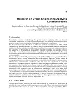
The concepts of fuzzy numbers are used to evaluate mainly the subjective attributes and
information related to importance of de general and specific factors.
Figure 1 presents the membership functions of the linguistic ratings, and Fig. 2 presents the
membership functions for linguistic values.
Fig. 1. Linguistic ratings: W = Weak: (0, 0.2, 0.2, 0.5), F = Fair: (0.17, 0.5, 0.5, 0.84), G = Good:
(0.5, 0.8, 0.8, 1), Ex = Excellent (0.8, 1, 1, 1)
1
f
R
0 0.2 0.4 1.0 R
irrelevant
1
f
R
0 0.3 0.5 0.7 1.0 R
nvc
1
f
R
0 0.6 0.8 1.0 R
conditional
1
f
R
0 0.8 1.0 R
critical
Fig. 2 Linguistic values: I = Irrelevant: (0, 0.2, 0.2, 0.4) , NVC = Not Very Conditional: (0.3,

0.5, 0.5, 0.7), C = Conditional: (0.6, 0.8, 0.8, 1.0), C = Critical : (0.8, 1.0, 1.0 , 1.0)
4. Methodology
The methodological approach consists in selecting a set of location factors that can be
measured in territorial sites and associated to characteristics of under study projects. The
offer and demand levels of these location factors must be defined and quantified, and a
fuzzy algorithm operates the datasets obtained, in order to produce a hierarchical indication
for sites and project location (Fig. 3).
The first step consists in listing appropriate location factors as resulting from territorial
study and project research. Territorial study also help on site contours adopted for offer
measurement, in general the suitable for available thematically data (economics, population,
etc.), such as municipal or district census boundaries. Project research describe what kind
and amount of facilities, resources, and logistics are necessary to improve related services
and activities. The initial information is used for classifying offer and demand in several
levels, corresponding to linguistic variables mentioned before in the mathematical model.
Methods and Techniques in Urban Engineering
78
b
jk
(Degrees for the k
i
alternatives)
FACTORS
B
1
B
2
B
3
a
ij

(Importance for
possibilities)
f
1
Weak Weak Excellent Conditional
f
2
Weak Good Good Critical
f
3
Good Good Good Critical
f
4
Weak Good Good Not very conditional
f
5
Fair Weak Weak Irrelevant
f
6
Excellent Good Excellent Conditional
f
7
Good Excellent Good Critical
a
ij
: fuzzy coefficient of the degree of importance of factor j related to the i project, and
b
jk
: fuzzy coefficient that results from the level of the factor related to the k area
Table 6. Example of degrees and weights for the i project

Assuming A*= (a*
ij
)
mxn’,
the demand matrix of i types of project related to n' specific location
factors. Concerning the use of the A matrix, all factors are critical, and for the activities
concerning raw materials, these characteristics can be defined by means of the results:
1. Relation product weight / raw material weight
2. Perishable raw materials
3. Relation factor freight / product freight
4. Relation freight factor / factor cost, etc
~
A
* = {f, µ
~
* ( )
A
f F
∈
} is the fuzzy representation of the A* matrix.
Assuming B* = [bij]
n’.m
the territorial supplying matrix of n' specific location factors of i kind
of project, concerning specific resources or any other specific conditioning factor, and Γ =
[γ
ik
]
mxq
= C ⊕ C*, where the aggregation of values (gamma operation) concerning the
activities on specific resources is achieved by Table 7 (with

~
c
ik
= fuzzy coefficient).

~
c
ik
>0 0
0 0 0
~
c
*
ik
>0 c
ik
+c*
ik
c*
ik
Table 7. Aggregation operator
The A = [ λ
ij
]
mxn
∑
matrix results from that defines the demand profile for the location effect,
where: n
∑
= n + n'.

Assuming � = (e
il
)
h x h
is the diagonal matrix, so that e
il
=
⎪
⎩
⎪
⎨
⎧
≠
∑
Σ
=
l=iif,a1/
liif,0
n
1
ij
j
∆ = [e x F] = [ δ
ik
] can still be defined as the representative matrix of the location possibilities
of the h types of projects in the m alternatives, now represented by indices related to
Research on Urban Engineering Applying Location Model
79
demanded location factors. That means that each element δ
ik

of the ∆ matrix represents the
indices of factors satisfied in the location of the i kind of projects in the k elementary zone.
If δ
ik
= 1 the k area satisfies the demand at the required level.
If δ
ik
< 1 means that at least one demanded factor was not satisfied.
If δ
ik
> 1 the k area offers more conditions than those demanded.
The concepts of fuzzy numbers are used to evaluate mainly the subjective attributes and
information related to importance of de general and specific factors.
Figure 1 presents the membership functions of the linguistic ratings, and Fig. 2 presents the
membership functions for linguistic values.
Fig. 1. Linguistic ratings: W = Weak: (0, 0.2, 0.2, 0.5), F = Fair: (0.17, 0.5, 0.5, 0.84), G = Good:
(0.5, 0.8, 0.8, 1), Ex = Excellent (0.8, 1, 1, 1)
1
f
R
0 0.2 0.4 1.0 R
irrelevant
1
f
R
0 0.3 0.5 0.7 1.0 R
nvc
1
f
R

0 0.6 0.8 1.0 R
conditional
1
f
R
0 0.8 1.0 R
critical
Fig. 2 Linguistic values: I = Irrelevant: (0, 0.2, 0.2, 0.4) , NVC = Not Very Conditional: (0.3,
0.5, 0.5, 0.7), C = Conditional: (0.6, 0.8, 0.8, 1.0), C = Critical : (0.8, 1.0, 1.0 , 1.0)
4. Methodology
The methodological approach consists in selecting a set of location factors that can be
measured in territorial sites and associated to characteristics of under study projects. The
offer and demand levels of these location factors must be defined and quantified, and a
fuzzy algorithm operates the datasets obtained, in order to produce a hierarchical indication
for sites and project location (Fig. 3).
The first step consists in listing appropriate location factors as resulting from territorial
study and project research. Territorial study also help on site contours adopted for offer
measurement, in general the suitable for available thematically data (economics, population,
etc.), such as municipal or district census boundaries. Project research describe what kind
and amount of facilities, resources, and logistics are necessary to improve related services
and activities. The initial information is used for classifying offer and demand in several
levels, corresponding to linguistic variables mentioned before in the mathematical model.
Methods and Techniques in Urban Engineering
80
Territorial Study
Project Research
Sites
Location Factors
Activities and Services
Offer dataset

Demand dataset
Offer x Demand
Fuzzy Operator
Location
Hierarchy
Fig. 3. Methodology
The offer is measured in levels for each considered site, and a geoprocessing tool can turn
this job more effective and precise. A geographic code is used as key column for relational
operations with the studied sites, as join and relates with tables containing thematic data.
The number of levels can vary from 4 (four) to 10 (ten), more levels are better for classifying
and displaying data in GIS ambient, but later they will must be regrouped in 4 (four) levels
(Cosenza & Lima, 1991) to attempt the linguistic concept (Excellent - Good - Fair – Weak).
The rules for converting data in operational values to indicate these levels are previously
defined in registry tables (relations between parameters and concepts) and could be
generated by geoprocessing tools in two ways:
 Spatial analyses, when properties as distance or pertinence to georeferenced items
(roads, pipelines, ports, plants, etc) are used to assign the level (Fig. 4),
 Statistic classification, when data is directly associated to the site contours (population,
incomes, etc), and a range of values must be classified by statistics and grouped as
assigned levels (Fig. 5).
Fig. 4. Georeferenced levels of highway infrastructure offer performed by spatial analyses
Research on Urban Engineering Applying Location Model
81
Fig. 5. Georeferenced levels of human development index offer performed by statistic classification
The demand is also organized in registry tables (Table 8), whose values are assigned by
subjective interpretation of experts, based in their experience on implementing and
operating similar projects. The more dependent projects are on a given factor; the highest is
the demand level assignment. The demand levels can be defined in a different number them
offer levels, but 4 (four) levels could deal more properly with the linguistic concept (Critical
- Conditional - Not very conditional – Irrelevant).

The factors must be defined on each project as general (G) or specific (S). As seen before, a
specific factor is more impacting than a general factor, because less offer of specific factor
(natural resources, climate, market, etc) them requested by project could harm the location.
Table 8. Demand table: project (identity preserved) in columns, location factors in lines
After assigned, both offer and demand datasets could be inputted as arrays and processed
by computational resources, that compare offer vs. demand relations for each site and each
project, in order to produce an output array containing hierarchical indicators.
Methods and Techniques in Urban Engineering
80
Territorial Study
Project Research
Sites
Location Factors
Activities and Services
Offer dataset
Demand dataset
Offer x Demand
Fuzzy Operator
Location
Hierarchy
Fig. 3. Methodology
The offer is measured in levels for each considered site, and a geoprocessing tool can turn
this job more effective and precise. A geographic code is used as key column for relational
operations with the studied sites, as join and relates with tables containing thematic data.
The number of levels can vary from 4 (four) to 10 (ten), more levels are better for classifying
and displaying data in GIS ambient, but later they will must be regrouped in 4 (four) levels
(Cosenza & Lima, 1991) to attempt the linguistic concept (Excellent - Good - Fair – Weak).
The rules for converting data in operational values to indicate these levels are previously
defined in registry tables (relations between parameters and concepts) and could be
generated by geoprocessing tools in two ways:

 Spatial analyses, when properties as distance or pertinence to georeferenced items
(roads, pipelines, ports, plants, etc) are used to assign the level (Fig. 4),
 Statistic classification, when data is directly associated to the site contours (population,
incomes, etc), and a range of values must be classified by statistics and grouped as
assigned levels (Fig. 5).
Fig. 4. Georeferenced levels of highway infrastructure offer performed by spatial analyses
Research on Urban Engineering Applying Location Model
81
Fig. 5. Georeferenced levels of human development index offer performed by statistic classification
The demand is also organized in registry tables (Table 8), whose values are assigned by
subjective interpretation of experts, based in their experience on implementing and
operating similar projects. The more dependent projects are on a given factor; the highest is
the demand level assignment. The demand levels can be defined in a different number them
offer levels, but 4 (four) levels could deal more properly with the linguistic concept (Critical
- Conditional - Not very conditional – Irrelevant).
The factors must be defined on each project as general (G) or specific (S). As seen before, a
specific factor is more impacting than a general factor, because less offer of specific factor
(natural resources, climate, market, etc) them requested by project could harm the location.
Table 8. Demand table: project (identity preserved) in columns, location factors in lines
After assigned, both offer and demand datasets could be inputted as arrays and processed
by computational resources, that compare offer vs. demand relations for each site and each
project, in order to produce an output array containing hierarchical indicators.
Methods and Techniques in Urban Engineering
82
To rule the process is used a relationship table (Table 9), where an equal offer vs. demand
diagonal is placed with value = 1, which represents situations that offer matches demand.
The other values could represent lack or excess, and may be adjusted to minimize or
maximize effects around diagonal. For instance, when a project still considers sites where a
little lack of offer as not critical, it could be assigned values near zero for poor offer relations,
if lack of offer cancel the project, all values where offer is less than demand should be zero.

In other way, when is interesting to know sites with a greater amount of offer, it could be
assigned an increment for best offer relations.
Table 9. Relationship table for offer vs. demand comparison and attributes: on columns weak, fair, good
and excellent; on lines irrelevant, not very conditional, conditional and critical
The results are obtained as a table (Table 10), where columns are projects and lines are sites,
and the obtained values express how territorial conditions match project requirements. A
value normalized to 1 (one) represents the situation where both offer and demand are
balanced, so location is recommended. Values greater than 1 (one) indicates that the site has
more offer conditions than required, and values less than 1 (one) indicates that at least one
of the factors was not attempted.
Table 10. Hierarchies location results for a set of municipalities, where project (identity preserved) is
placed in columns, with last column shows media for all projects
Table could be now georeferenced to the sites (Fig. 6) by their geographic codes, using join
or relate operations with the georeferenced tables. In the next step, location indicators are
classified by statistics and displayed as chromatic conventions, in order to interpret spatial
possibilities of placement. The chromatic classification for results can use various statistic
methods, such as: natural breaks, equal interval, standard derivation and quantile.
Research on Urban Engineering Applying Location Model
83
Fig. 6. Location indicators are classified and displayed as chromatic conventions
Natural breaks are indicated to group a set of values between break points that identifies a
change in distribution patterns, and is the most frequent used form of visualization for
identifying best location. Equal interval is used to divide the range into equal size values
sub-ranges, and is used to identify results perform in comparison analysis. Standard
derivation is used to indicate how a value varies from the mean, and is often used to show
how results are dispersed. Quantile groups the set of values in equal number of items, and is
used less frequently because results are normalized.
7. Conclusion
Location models can also be employed for previewing land use and occupation of urban
areas. An analogy could be done considering an occupation typology (habitational

buildings, industrial zone, etc.) as a project for an urban site (district, zone, land, etc.). A list
of location factors that direct urban development could be selected from spatial, economic
and social data records (population, market, education, prices, mobility, health care, etc.).
The offer of these location factors could be measured on urban sites from local surveys or
official census data. Most of geographic offices in charge of registering official data make
available their operational boundaries as feature classes compatible with GIS platforms.
Urban planners, engineers, public services managers, political authorities, should define the
demand set, and will determinate the relevance of a factor on occupation typology, and
multi criteria analysis will be helpful to equalize their opinion (Liang & Wang, 1991).
But how a location model can help urban engineering research? If a land use or activity
placement could be treated as a project, ordering distinct location factors, it should be
possible to measure territorial offer and typology demand. Presuming that recent placement
situations can be studied to produce diagnosis based on configuration of related offer and
demand sets, researching past offer sets may be interesting for understanding how factors
evolution influences a site.
Methods and Techniques in Urban Engineering
82
To rule the process is used a relationship table (Table 9), where an equal offer vs. demand
diagonal is placed with value = 1, which represents situations that offer matches demand.
The other values could represent lack or excess, and may be adjusted to minimize or
maximize effects around diagonal. For instance, when a project still considers sites where a
little lack of offer as not critical, it could be assigned values near zero for poor offer relations,
if lack of offer cancel the project, all values where offer is less than demand should be zero.
In other way, when is interesting to know sites with a greater amount of offer, it could be
assigned an increment for best offer relations.
Table 9. Relationship table for offer vs. demand comparison and attributes: on columns weak, fair, good
and excellent; on lines irrelevant, not very conditional, conditional and critical
The results are obtained as a table (Table 10), where columns are projects and lines are sites,
and the obtained values express how territorial conditions match project requirements. A
value normalized to 1 (one) represents the situation where both offer and demand are

balanced, so location is recommended. Values greater than 1 (one) indicates that the site has
more offer conditions than required, and values less than 1 (one) indicates that at least one
of the factors was not attempted.
Table 10. Hierarchies location results for a set of municipalities, where project (identity preserved) is
placed in columns, with last column shows media for all projects
Table could be now georeferenced to the sites (Fig. 6) by their geographic codes, using join
or relate operations with the georeferenced tables. In the next step, location indicators are
classified by statistics and displayed as chromatic conventions, in order to interpret spatial
possibilities of placement. The chromatic classification for results can use various statistic
methods, such as: natural breaks, equal interval, standard derivation and quantile.
Research on Urban Engineering Applying Location Model
83
Fig. 6. Location indicators are classified and displayed as chromatic conventions
Natural breaks are indicated to group a set of values between break points that identifies a
change in distribution patterns, and is the most frequent used form of visualization for
identifying best location. Equal interval is used to divide the range into equal size values
sub-ranges, and is used to identify results perform in comparison analysis. Standard
derivation is used to indicate how a value varies from the mean, and is often used to show
how results are dispersed. Quantile groups the set of values in equal number of items, and is
used less frequently because results are normalized.
7. Conclusion
Location models can also be employed for previewing land use and occupation of urban
areas. An analogy could be done considering an occupation typology (habitational
buildings, industrial zone, etc.) as a project for an urban site (district, zone, land, etc.). A list
of location factors that direct urban development could be selected from spatial, economic
and social data records (population, market, education, prices, mobility, health care, etc.).
The offer of these location factors could be measured on urban sites from local surveys or
official census data. Most of geographic offices in charge of registering official data make
available their operational boundaries as feature classes compatible with GIS platforms.
Urban planners, engineers, public services managers, political authorities, should define the

demand set, and will determinate the relevance of a factor on occupation typology, and
multi criteria analysis will be helpful to equalize their opinion (Liang & Wang, 1991).
But how a location model can help urban engineering research? If a land use or activity
placement could be treated as a project, ordering distinct location factors, it should be
possible to measure territorial offer and typology demand. Presuming that recent placement
situations can be studied to produce diagnosis based on configuration of related offer and
demand sets, researching past offer sets may be interesting for understanding how factors
evolution influences a site.
Methods and Techniques in Urban Engineering
84
For instance, registering and analyzing the offer records along a significant time, and
consulting specialists for demand attribute, it will be possible to isolate pattern
characteristics of a situation. Observing offer increase or decrease along the time, a general
urban evolution tendency (residential, industrial, commercial, etc.) could be expressed by its
particular demand set. Comparing the urban site offer with a demand assigned pattern, it is
possible by simulation to explore future scenarios. A georeferenced array of urban sites vs.
pattern characteristics could indicate how intense each site matches the pattern
characteristics, and based on the values obtained verify the possibilities of occurrence.
So, if the responsible authority inquires about a place that would be a commercial zone in
the next five years, the researcher would construct an offer fuzzy set of the urban site based
on recent data, and check it with a proposed pattern of typical commercial zone factors
demand. The possibility of occurrence, defined by the hierarchic values, could be used to
determinate and prioritize actions.
By extracting specific geodata of offer and demand sets, it is also possible to identify which
factors have significant influence on the results, and so define strategic intervention that
could direct the expected results.
To conclude, an offer and demand logic operator attached to geoprocessing resources could
enhance the horizon of researches on urban engineering methods, and improve queries and
simulations that will help to understand and simulate the dynamic of cities growth.
8. References

Attanasio, D. & alii, (1974).
Masterlli-

Modelo di Assetto Territoriale e di Localizzazione
Industriale
, Centro Studi Confindustria, Bologna
Attanasio, D. (1976).
Fattori de Localizzazione nell’Industria Manufatturiera
, Centro Studi
Confindustria, Bologna
Cosenza, C. (1981).
A Industrial Location Model
, Working Paper, Martin Centre for
Architctural and Urban Studies, Cambridge University, Cambridge
Cosenza, C. & Lima, F. (1991). Aplicação de um Modelo de Hierarquização de Potenciais de
Localização no Zoneamento Industrial Metropolitano: Metodologia para
mensuração de Oferta e Demanda de Fatores Locacionais,
Proceedings of V ICIE -
International Congress of Industrial Engineering,
ABEPRO, Rio de Janeiro
Curry, B. & Moutinho, L. (1992). Computer Models for Site Location Decisions,
International
Journal of Retail & Distribution Management
., Vol. 20
Harlow, M. (2005).
ArcGIS Reference Documentation
, ESRI: Environmental Systems
Research Institute Inc., Redlands
Jarboe, K. (1986). Location decisions on high-technology firms: A case study,
Technovation,

Vol. 4, pp. 117-129
Kahraman, C. & Dogan, L. (2003). Fuzzy Group decision-making for Facility Location
Selection,
Information Sciences
, p. 157, University of California, Berkley
Liang. G. & Wang, M. (1991). A Fuzzy Multi-Criteria Decision-Making Method for Facility
Site Selection.
Int. J. Prod. Res.,
Vol. 29, No. 11, pp. 2313-2330
Lima, F., Cosenza, C. & Neves, C. (2006). Estudo de Localização para as Atividades de
Produção do Biodiesel da Mamona no Nordeste Empregando Sistemas de
Informação Georeferenciados,
Proceedings of XI Congresso Brasileiro de Energia
,
Vol. II, pp. 661-668, COPPE/UFRJ, Rio de Janeiro
SpatialAnalysisforIdentifyingConcentrationsofUrbanDamage
JosephWartman,NicholasE.Malasavage
7
Spatial Analysis for Identifying Concentrations
of Urban Damage
Joseph Wartman, Nicholas E. Malasavage
Drexel University Engineering Cities Initiative (DECI)
,
United States of America
1. Introduction
Disasters resulting from earthquakes, hurricanes, fires, floods, and terrorist attacks can
result in significant and highly concentrated damage to buildings and infrastructure within
urban regions. Following such events, it is common to dispatch investigation teams to
catalog and inventory damage locations. In recent years, these data gathering efforts have
been aided by developments in high resolution satellite remote sensing technologies (e.g.

Matsuoka & Yamazaki, 2005) and by advances in ground-based field data collection (e.g.
Deaton & Frost, 2002). Damage inventories are typically presented as maps showing the
location and damage state of structures in part or all of an effected region. In some cases
information on the post-event condition of major infrastructure systems such as
transportation, power, communications, and water networks is also included. Depending on
the means used to acquire data, damage inventories may be developed in days (satellite-
based data acquisition) or weeks-to-months (ground-based damage surveys) after an event.
Once available, these inventories can be used for a range of purposes including guiding
emergency rescues (short-term use), identification of neighborhoods requiring post-disaster
financial assistance (intermediate-term use), and support of zoning, planning or urban
policy studies (long-term use). An important task when analyzing these inventories is to
identify and quantify damage concentrations or clusters, as this information is useful for
prioritizing post-disaster recovery activities. Additionally, an understanding of damage
concentrations can provide insight to the multiscale processes that govern an urban region's
performance during an extreme event.
In some cases spatial patterns and clusters can be inferred from damage inventories using
simple, qualitative visual assessment techniques. While this may be a satisfactory approach
in situations where there is a marked contrast in building performance, its effectiveness is
limited when damage contrasts are subtle, and spatial patterns are less obvious. In these
instances, more advanced spatial analysis tools such as point pattern analysis can be of
benefit.
Point pattern analysis (PPA) techniques are a group of quantitative methods that describe
the pattern of point (or
event
) locations and determine if point locations are concentrated (or
clustered
) within a defined region of study. An early and often-cited example of a semi-
7
Methods and Techniques in Urban Engineering
86

qualitative application of the PPA concept is physician John Snow's mid-nineteenth century
investigation of a cholera outbreak in London (Johnson, 2006). By mapping the locations of
drinking water pumps along with the residences of individuals suffering cholera-related
illness, Snow was able to link the epidemic to the local water supply. More recently, a
rigorous statistical framework for PPA has largely emerged from work within the plant
ecology research community. Since the advent of Geographical Information Systems (GIS),
PPA has been used with increasing frequency in a range of applications including
identification of crime patterns (e.g. Ratcliffe & McCullagh, 1999) and tracking of disease
outbreaks (e.g. Lai et al., 2004).
This chapter will review methods from three classes of PPA within the context of an
assessment of a high quality building damage inventory. The mathematical formulation of
PPA methods have been discussed in detail elsewhere (e.g. Diggle, 2003; Wong & Lee, 2005;
Illian et al. 2008) and therefore will not be repeated here. Instead, this chapter will focus on
the
application
of PPA techniques and the
interpretation
of results for an urban damage
inventory compiled after the 2001 Southern Peru earthquake. Results of the analyses will be
compared and discussed along with other pertinent issues. In fitting with the theme of this
volume, this chapter is intended to give readers less familiar with spatial analysis a basic
framework for understanding key concepts of PPA. More detailed discussions of the
techniques discussed in this chapter can be found in Fotheringham et al. (2000), O'Sullivan
& Unwin (2003), Fortin & Dale (2005), Mitchell (2005) and Pfeiffer et al. (2008), among other
excellent references. Although the chapter is geared toward urban damage inventories, the
concepts presented here are appropriate for a wide range of applications in urban
engineering and policy (Table 1). Thus it is hoped that this work will inspire more frequent
and innovative use of spatial analyses in urban engineering practice and research.
Discipline Points/Events Application
Infrastructure

Engineering
Underground service
repairs
Plan/prioritize maintenance and
future upgrades to system
Infrastructure
Engineering
Manufacturing centers
Site specific municipal services
facilities such as recycling centers
Transportation
Engineering
Automobile
accidents/pedestrian
incidents
Identify roads and intersections
requiring safety enhancements
Transportation
Engineering
Persons
Siting of
transit hubs and connections
Environmental
Engineering
Environmental
monitoring locations
Identify and track pollution point
sources
Civil Engineering Landslides Hazard zonation
Public health

Water-borne disease
outbreaks
Drinking water quality evaluation
Environmental
Science
Urban wildlife sightings
Assess wildlife nesting or
migration habits
Table 1. Example of applications of PPA in Urban Engineering and Policy Making
Spatial Analysis for Identifying Concentrations of Urban Damage
87
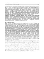
2. Case Study of Damage in San Francisco (Moquegua, Peru) during the 2001
Southern Peru Earthquake
2.1 Overview
The 23 June 2001 moment magnitude (M
w
) 8.4 Southern Peru earthquake affected a
widespread area that included several important population centers in southern Peru and
northern Chile, including Moquegua, the city that will be the focus of this chapter (Figure 1).
The earthquake occurred along the active subduction boundary of the Nazca and the South
American plates resulting in widespread damage throughout the region. In general, adobe
buildings and older structures were most susceptible to damage, though a significant
number of modern engineered structures were also impacted by the earthquake. Rodriguez-
Marek and Edwards (2003) present a comprehensive overview of the damage caused by the
earthquake. Only a limited number of strong motion instruments recorded the main shock,
with the largest peak ground acceleration of 0.33 g being measured in the northern Chilean
city of Arica. The only ground motion station in Peru, coincidentally located in the city of
Moquegua, registered a moderately high peak ground acceleration of 0.30 g.
-75 -74 -73 -72 -71 -70
Longitude

-19
-18
-17
-16
Latitude
Pacific Ocean
Chile
Tacna
Moquegua
Peru
Arequipa
Camana
Ilo
Legend
town
epicenter
zone of maximum
energy release
study area
Peru
50 km
Fig. 1. Regional map showing the location urban centers impacted by the 2001 Southern
Peru earthquake
The city of Moquegua (population: 60,000) is situated in an alluvial valley at the base of the
Andes Mountains. The city is located approximately 55 km east of the Pacific coast at an
elevation of 1400 meters. San Francisco, an approximately 1 km
2
neighborhood located in
the southwestern part of Moquegua, was one of the most damaged areas in the city (Figures
2 and 3). In contrast to most of Moquegua, which is relatively flat, San Francisco is

distinguished by its variation in topography (Figure 4). San Francisco is situated on a
geologic outcrop that includes three ridges rising roughly 100 m above the surrounding
portions of the city. This outcrop, which daylights in the upper half of each ridge, consists of
stiff conglomerate of the Moquegua geologic formation. This outcrop is also the primary
source of alluvium and colluvium that forms a soil mantle that generally thickens with
Methods and Techniques in Urban Engineering
86
qualitative application of the PPA concept is physician John Snow's mid-nineteenth century
investigation of a cholera outbreak in London (Johnson, 2006). By mapping the locations of
drinking water pumps along with the residences of individuals suffering cholera-related
illness, Snow was able to link the epidemic to the local water supply. More recently, a
rigorous statistical framework for PPA has largely emerged from work within the plant
ecology research community. Since the advent of Geographical Information Systems (GIS),
PPA has been used with increasing frequency in a range of applications including
identification of crime patterns (e.g. Ratcliffe & McCullagh, 1999) and tracking of disease
outbreaks (e.g. Lai et al., 2004).
This chapter will review methods from three classes of PPA within the context of an
assessment of a high quality building damage inventory. The mathematical formulation of
PPA methods have been discussed in detail elsewhere (e.g. Diggle, 2003; Wong & Lee, 2005;
Illian et al. 2008) and therefore will not be repeated here. Instead, this chapter will focus on
the
application
of PPA techniques and the
interpretation
of results for an urban damage
inventory compiled after the 2001 Southern Peru earthquake. Results of the analyses will be
compared and discussed along with other pertinent issues. In fitting with the theme of this
volume, this chapter is intended to give readers less familiar with spatial analysis a basic
framework for understanding key concepts of PPA. More detailed discussions of the
techniques discussed in this chapter can be found in Fotheringham et al. (2000), O'Sullivan

& Unwin (2003), Fortin & Dale (2005), Mitchell (2005) and Pfeiffer et al. (2008), among other
excellent references. Although the chapter is geared toward urban damage inventories, the
concepts presented here are appropriate for a wide range of applications in urban
engineering and policy (Table 1). Thus it is hoped that this work will inspire more frequent
and innovative use of spatial analyses in urban engineering practice and research.
D
iscipline Points/Events Application
Infrastructure
Engineering
Underground service
repairs
Plan/prioritize maintenance and
future upgrades to system
Infrastructure
Engineering
Manufacturing centers
Site specific municipal services
facilities such as recycling centers
Transportation
Engineering
Automobile
accidents/pedestrian
incidents
Identify roads and intersections
requiring safety enhancements
Transportation
Engineering
Persons
Siting of
transit hubs and connections

Environmental
Engineering
Environmental
monitoring locations
Identify and track pollution point
sources
Civil Engineering Landslides Hazard zonation
Public health
Water-borne disease
outbreaks
Drinking water quality evaluation
Environmental
Science
Urban wildlife sightings
Assess wildlife nesting or
migration habits
Table 1. Example of applications of PPA in Urban Engineering and Policy Making
Spatial Analysis for Identifying Concentrations of Urban Damage
87
2. Case Study of Damage in San Francisco (Moquegua, Peru) during the 2001
Southern Peru Earthquake
2.1 Overview
The 23 June 2001 moment magnitude (M
w
) 8.4 Southern Peru earthquake affected a
widespread area that included several important population centers in southern Peru and
northern Chile, including Moquegua, the city that will be the focus of this chapter (Figure 1).
The earthquake occurred along the active subduction boundary of the Nazca and the South
American plates resulting in widespread damage throughout the region. In general, adobe
buildings and older structures were most susceptible to damage, though a significant

number of modern engineered structures were also impacted by the earthquake. Rodriguez-
Marek and Edwards (2003) present a comprehensive overview of the damage caused by the
earthquake. Only a limited number of strong motion instruments recorded the main shock,
with the largest peak ground acceleration of 0.33 g being measured in the northern Chilean
city of Arica. The only ground motion station in Peru, coincidentally located in the city of
Moquegua, registered a moderately high peak ground acceleration of 0.30 g.
-75 -74 -73 -72 -71 -70
Longitude
-19
-18
-17
-16
Latitude
Pacific Ocean
Chile
Tacna
Moquegua
Peru
Arequipa
Camana
Ilo
Legend
town
epicenter
zone of maximum
energy release
study area
Peru
50 km
Fig. 1. Regional map showing the location urban centers impacted by the 2001 Southern

Peru earthquake
The city of Moquegua (population: 60,000) is situated in an alluvial valley at the base of the
Andes Mountains. The city is located approximately 55 km east of the Pacific coast at an
elevation of 1400 meters. San Francisco, an approximately 1 km
2
neighborhood located in
the southwestern part of Moquegua, was one of the most damaged areas in the city (Figures
2 and 3). In contrast to most of Moquegua, which is relatively flat, San Francisco is
distinguished by its variation in topography (Figure 4). San Francisco is situated on a
geologic outcrop that includes three ridges rising roughly 100 m above the surrounding
portions of the city. This outcrop, which daylights in the upper half of each ridge, consists of
stiff conglomerate of the Moquegua geologic formation. This outcrop is also the primary
source of alluvium and colluvium that forms a soil mantle that generally thickens with
Methods and Techniques in Urban Engineering
88
decreasing elevation. Soil thickness ranges from 0 m on the hillside, to approximately 6 m in
valley and flatland areas. San Francisco has grown continuously over the past 40 to 50 years
to its 2001 population of 12,000. Buildings in the neighborhood are primarily of masonry or
similar construction, with a lesser number of older adobe structures. A summary of land use
in San Francisco is presented in Table 2.
Fig. 2. Aerial view of Moquegua showing the San Francisco neighborhood outlined in red. A
river is visible at north of the neighborhood. (via Google earth, North is vertical)
Fig. 3. Building damage in San Francisco after the 2001 Southern Peru earthquake
The absence of earthquake-induced ground failure (i.e., soil liquefaction and landslides) in
San Francisco suggested that the high levels of building damage were a result of strong
localized shaking. Several preliminary post-earthquake investigation reports (e.g. Kosaka-
Masuno et al., 2001; Kusunoki, 2002; Rodriguez-Marek et al., 2003) hypothesized that the
high levels of damage to were due to topographic amplification (Kramer 1996) of ground
motion, resulting in localized strong ground shaking. This phenomenon, where topographic
features (e.g. hills and ridges) alters and amplifies local ground shaking, has been observed

in past earthquakes and is most pronounced near ridge tops. Given the topography of San
Francisco, this was a plausible explanation; however, later published data suggested that
damage concentrations were located away from ridge tops, indicating that other factors may
Spatial Analysis for Identifying Concentrations of Urban Damage
89
have governed localized ground motion intensity in the neighborhood. A question then
remains: what role, if any, did topography play in the damage distribution in San Francisco?
This chapter will consider the topographic amplification question further by conducting a
series of analyses to determine if building damage in San Francisco was clustered and if so,
to see if the cluster locations coincide with areas of relief as would be expected with
topographic amplification.
Fig. 4. Street map and topography of San Francisco. The red lines indicate the locations of
ridgetops
L
and Use
Number of Land
Parcels
Percent of Land
Parcels
Residential 1611 76.4%
Commercial 89 4.2%
Government 89 4.2%
Vacant 320 15.2%
T
otal = 2190 100%
Table 2. Summary of land use in San Francisco
2.2 PREDES Damage Inventory
Several earthquake damage inventories for the region have been published, including a high
quality, comprehensive account produced by Peru’s Center for the Study and Prevention of
Disasters (PREDES, 2003). This inventory was developed as part of a larger effort by local

engineers, architects and social scientists to assess the effectiveness of short term disaster
200 Meters0
E
levation
(
m
)
1360
1470
Methods and Techniques in Urban Engineering
88
decreasing elevation. Soil thickness ranges from 0 m on the hillside, to approximately 6 m in
valley and flatland areas. San Francisco has grown continuously over the past 40 to 50 years
to its 2001 population of 12,000. Buildings in the neighborhood are primarily of masonry or
similar construction, with a lesser number of older adobe structures. A summary of land use
in San Francisco is presented in Table 2.
Fig. 2. Aerial view of Moquegua showing the San Francisco neighborhood outlined in red. A
river is visible at north of the neighborhood. (via Google earth, North is vertical)
Fig. 3. Building damage in San Francisco after the 2001 Southern Peru earthquake
The absence of earthquake-induced ground failure (i.e., soil liquefaction and landslides) in
San Francisco suggested that the high levels of building damage were a result of strong
localized shaking. Several preliminary post-earthquake investigation reports (e.g. Kosaka-
Masuno et al., 2001; Kusunoki, 2002; Rodriguez-Marek et al., 2003) hypothesized that the
high levels of damage to were due to topographic amplification (Kramer 1996) of ground
motion, resulting in localized strong ground shaking. This phenomenon, where topographic
features (e.g. hills and ridges) alters and amplifies local ground shaking, has been observed
in past earthquakes and is most pronounced near ridge tops. Given the topography of San
Francisco, this was a plausible explanation; however, later published data suggested that
damage concentrations were located away from ridge tops, indicating that other factors may
Spatial Analysis for Identifying Concentrations of Urban Damage

89
have governed localized ground motion intensity in the neighborhood. A question then
remains: what role, if any, did topography play in the damage distribution in San Francisco?
This chapter will consider the topographic amplification question further by conducting a
series of analyses to determine if building damage in San Francisco was clustered and if so,
to see if the cluster locations coincide with areas of relief as would be expected with
topographic amplification.
Fig. 4. Street map and topography of San Francisco. The red lines indicate the locations of
ridgetops
Land Use
Number of Land
Parcels
Percent of Land
Parcels
Residential 1611 76.4%
Commercial 89 4.2%
Government 89 4.2%
Vacant 320 15.2%
Total = 2190 100%
Table 2. Summary of land use in San Francisco
2.2 PREDES Damage Inventory
Several earthquake damage inventories for the region have been published, including a high
quality, comprehensive account produced by Peru’s Center for the Study and Prevention of
Disasters (PREDES, 2003). This inventory was developed as part of a larger effort by local
engineers, architects and social scientists to assess the effectiveness of short term disaster
200 Meters0
Elevation
(
m
)

1360
1470
Methods and Techniques in Urban Engineering
90
response in the neighborhood. The PREDES survey was based on individual inspections of
close to 1900 buildings whose seismic performance was rated as good, moderate or poor,
corresponding to buildings that exhibited no significant damage, significant cracks to
loading bearing members, and collapse, respectively. The survey also categorized each
building according to its typology (Table 3), as this is known to be an important factor
governing the seismic performance of structures. Buildings comprised of masonry and
"mixed" construction (i.e., combined masonry and adobe materials) are widely recognized to
be of higher construction quality (and seismic resistance) than adobe dwellings.
Percentage of Buildings
Exhibiting Damage
Building Type
Low Moderate High
No. of
Buildings
(% of Study)
Masonry 81.7% 16.5% 1.8% 968 (52.0%)
Mixed 31.2% 56.6% 12.2% 548 (29.5%)
Adobe 2.6% 21.8% 75.6% 344 (18.5%)
Table 3. Building typology and damage statistics for San Francisco
Figure 5 shows the locations of buildings in San Francisco and their respective typologies.
The open areas in the northwest corner of the study area are the locations of two
undeveloped land parcels. The study zone was defined to include only the areas where
complete data was available for all buildings. This was required because a full data
inventory (rather than a sampling) is needed to properly conduct a PPA. Figure 6 shows the
post-earthquake damage state of each building in the study area.
Fig. 5. Building locations and typologies in San Francisco (after PREDES, 2003)

200 Meters0
Mixed
Masonry
Adobe
Spatial Analysis for Identifying Concentrations of Urban Damage
91
Fig. 6. Post-earthquake damage condition for all structures located in San Francisco (after
PREDES, 2003)
Review of Figures 5 and 6 along with the data included in Table 3 indicates the following:
 With some minor exceptions related to a concentration of mixed dwellings located in
the south-central portion of San Francisco, the building types appear to be generally
well distributed throughout the neighborhood. Most streets are characterized by
interspersed masonry, mixed, and adobe dwellings.
 A majority of the buildings in San Francisco are of masonry or mixed construction.
 Overall, a majority of the higher quality (i.e., masonry and mixed structures) buildings
in the neighborhood performed well (“low” damage intensity) in the earthquake. In
contrast, the seismic performance of nearly all of the adobe structures was poor (“high”
damage intensity).
 It is difficult to identify any clear patterns on concentrations of damage from the overall
damage survey using visual assessment alone.
The combination of different building types and performance levels make the damage
inventory quite complex when considered in aggregate. Although advanced multivariate
statistical techniques could be used to analyze the data, PPA provides a more direct
approach tailored to the principal objective of the study (i.e., identification of damage
clusters). However, this technique requires consistency in the database and thus the
PREDES data inventory was modified to ensure uniform building construction quality.
Specifically, adobe buildings, which have significantly lower seismic resistance than
masonry and mixed structures, were not considered. As these comprised only a small
fraction of the total building inventory, this did not significantly reduce the total number of
buildings in the inventory. The performance of the remaining 1,513 buildings in the

inventory (i.e., masonry and mixed structures) was re-categorized in a binary manner as “no
200 Meters0
D
amage Intensity
Moderate
Low
Hi
g
h
Methods and Techniques in Urban Engineering
90
response in the neighborhood. The PREDES survey was based on individual inspections of
close to 1900 buildings whose seismic performance was rated as good, moderate or poor,
corresponding to buildings that exhibited no significant damage, significant cracks to
loading bearing members, and collapse, respectively. The survey also categorized each
building according to its typology (Table 3), as this is known to be an important factor
governing the seismic performance of structures. Buildings comprised of masonry and
"mixed" construction (i.e., combined masonry and adobe materials) are widely recognized to
be of higher construction quality (and seismic resistance) than adobe dwellings.
P
ercentage of Buildings
Exhibiting Damage
Building Type
Low Moderate High
No. of
Buildings
(% of Study)
Masonry 81.7% 16.5% 1.8% 968 (52.0%)
Mixed 31.2% 56.6% 12.2% 548 (29.5%)
Adobe 2.6% 21.8% 75.6% 344 (18.5%)

Table 3. Building typology and damage statistics for San Francisco
Figure 5 shows the locations of buildings in San Francisco and their respective typologies.
The open areas in the northwest corner of the study area are the locations of two
undeveloped land parcels. The study zone was defined to include only the areas where
complete data was available for all buildings. This was required because a full data
inventory (rather than a sampling) is needed to properly conduct a PPA. Figure 6 shows the
post-earthquake damage state of each building in the study area.
Fig. 5. Building locations and typologies in San Francisco (after PREDES, 2003)
200 Meters0
Mixed
Masonr
y
Adobe
Spatial Analysis for Identifying Concentrations of Urban Damage
91
Fig. 6. Post-earthquake damage condition for all structures located in San Francisco (after
PREDES, 2003)
Review of Figures 5 and 6 along with the data included in Table 3 indicates the following:
 With some minor exceptions related to a concentration of mixed dwellings located in
the south-central portion of San Francisco, the building types appear to be generally
well distributed throughout the neighborhood. Most streets are characterized by
interspersed masonry, mixed, and adobe dwellings.
 A majority of the buildings in San Francisco are of masonry or mixed construction.
 Overall, a majority of the higher quality (i.e., masonry and mixed structures) buildings
in the neighborhood performed well (“low” damage intensity) in the earthquake. In
contrast, the seismic performance of nearly all of the adobe structures was poor (“high”
damage intensity).
 It is difficult to identify any clear patterns on concentrations of damage from the overall
damage survey using visual assessment alone.
The combination of different building types and performance levels make the damage

inventory quite complex when considered in aggregate. Although advanced multivariate
statistical techniques could be used to analyze the data, PPA provides a more direct
approach tailored to the principal objective of the study (i.e., identification of damage
clusters). However, this technique requires consistency in the database and thus the
PREDES data inventory was modified to ensure uniform building construction quality.
Specifically, adobe buildings, which have significantly lower seismic resistance than
masonry and mixed structures, were not considered. As these comprised only a small
fraction of the total building inventory, this did not significantly reduce the total number of
buildings in the inventory. The performance of the remaining 1,513 buildings in the
inventory (i.e., masonry and mixed structures) was re-categorized in a binary manner as “no
200 Meters0
D
amage Intensity
Moderate
Low
High
Methods and Techniques in Urban Engineering
92
damage/moderate damage” and “collapse”. As collapsed buildings (rather than partially
damaged) were responsible for most of the injuries and fatalities in the earthquake, the PPA
was focused specifically on this damage category. Based on these refinements to the original
PREDES database, the point events for the PPA are thus defined as masonry and mixed
construction buildings (i.e., higher quality structures) that collapsed in the earthquake. The
locations of these damaged buildings, which comprise 5% of the structures in the refined
database, are shown in Figure 7. Visual inspection of this figure fails to reveal any marked
or otherwise obvious concentrations of collapsed buildings. This inventory of collapsed
buildings will be considered in a more quantitative manner in the following sections.
Fig. 7. Collapsed masonry and mixed buildings (shown in red) in San Francisco
3. Point Pattern Analysis (PPA) of Collapsed Building Locations in San
Francisco

3.1 Data Requirements for PPA
Point patterns consist of a series of spatially distributed points, or
events
. To constitute a
point pattern, a set of events must meet the five criteria highlighted below (O'Sullivan &
Unwin, 2003) and discussed in the context of the PREDES damage inventory:
1. The patterns should be mapped on a plane.
Owing to the topographic relief in San
Francisco, the events occur over a three-dimensional ground surface. Nevertheless,
variations in elevation (1360 m to 1470 m) are small relative to the plan dimensions of the
neighborhood (approximately 1000 m by 1300 m) and thus the study area can be reasonably
approximated as a plane.
2. The study area should be determined objectively, rather than arbitrarily.
The boundaries
of the San Francisco study area were delineated based on the availability of data; however,
200 Meters0
Spatial Analysis for Identifying Concentrations of Urban Damage
93
this area fully encompasses the major topographic features of the neighborhood and also
includes some of the surrounding flatlands. As such, the PPA can be used to determine if
clusters are associated with the neighborhood's topographic features.
3. The events must be based on a census of the study area, rather than a sampling.
The
PREDES inventory was developed based on detailed building-by-building (i.e. census-type)
inspections, thus satisfying this criterion.
4. Objects in the study area must directly correspond to events in the pattern.
The events
were defined so as to directly correspond to masonry and mixed construction buildings that
collapsed in the earthquake, thereby satisfying this criterion.
5. Event locations must be proper, rather than representative of a larger object.

The damage
event locations were taken as the centroid of a building lot; however, as these lots are
relatively small (approximately 180 m
2
) relative to the size of the study area (approximately
750,000 m
2
), this is judged to be a reasonable approach for estimating the event locations.
3.2 PPA techniques
There are three basic approaches for conducting a PPA. The first involves determining the
number of events within a given area and therefore are referred to as
density-based
methods. The simplest of this class of methods are quadrat counts, whereby quadrats are
drafted over the study area and the number of events in each is counted to determine
quadrat densities. A more sophisticated but conceptually similar density-based method
involves kernel density functions, whereby events are summed within a series of circular
regions centered at a given location within the study area. The second approach for PPA
involves the determination of distances between events, and is thus referred to as a
distance-
function
. The third approach to PPA considers
spatial associations that vary locally
from the
larger global trends across a region of study. As will be discussed below, most of these
approaches can be combined with statistical analysis to obtain more rigorous quantitative
description of point patterns and clustering.
3.2.1 Quadrat Count Methods
Quadrat counts are perhaps the simplest and easiest of the PPA techniques to understand
and use. With this method the intensity of a point pattern (
λ

) is computed as:
α
λ
n
=
(1)
Where
n
is the number of events within a quadrat and α is the area of individual equal
dimension quadrats imposed over the study area.
Figure 8 shows grids of 50 m, 100 m, and 150 m square quadrats over the study area. Each
grid was oriented in a north-south/east-west orientation, with the origin located at the
south-west limit of the neighborhood. It should be apparent that grid orientation can affect
the resulting quadrat counts, especially when larger grid sizes are used. The color intensity
on the figures is proportional to the number of points (events) in each quadrat. Note that the
value of the color scale varies between each of the three diagrams.