Methods and Techniques in Urban Engineering Part 13 pdf
Bạn đang xem bản rút gọn của tài liệu. Xem và tải ngay bản đầy đủ của tài liệu tại đây (851.66 KB, 20 trang )
Methods and Techniques in Urban Engineering
232
15. Lessons Learned
The construction of adequate public transport facilities is one of most problematic issues
when implementing a housing policy. As large investments are necessarily required, it is
safe to assume that considerable delays may be expected with negative pitfalls on the
quality of service. These problems can be averted if (private) public transport companies
were to be included at an earlier stage in the policy planning process.
Citizens’ participation is pivotal for creating mixed-use areas. The shaping of traditional
European cities leads to postulate that mixed-used areas are not the result of detailed
planning – as they are more the outcome of spontaneous development. According to this
assumption, self-organisation and citizens participation in developing mixed-used districts
(not only in the planning and building stage) is one of the preconditions for creating a
mixed-used area accepted by its inhabitants for a long time.
Shopping malls can compete with businesses located in well-integrated mixed-use city
centres. Well-situated customers prefer shopping in malls, but also distant shoppers accept
long travel distances, long travel time, as well as congestion in order to shop there.
Campaigns informing that time is not gained when driving to non-integrated shopping
centres in peak hours and public transport must be promoted to influence customers.
Location policies successfully regulate public and private investments and have strongly
strengthened the vitality of the cities. Firstly, they can concentrate public investments in
infrastructure and public transport within the urban areas. Secondly, they can start large
urban renewal programs to upgrade the inner city areas around major transport node urban
locations, and thirdly they help to attract private investments to the city. Especially the
strong development of locations reachable both by public transport and car can induce a
new economic impulse for the urban economy. To make a location policy successful, the
implementation of other transport policies and land use policies are necessary. The location
policy can only function well when included into a well-balanced policy package.
Furthermore, the success of this policy depends on the availability of all the accessibility
profiles. Refrain from creating new planning bodies.
While it is correct that the integration between land use and transportation planning is in its
essence a regional task, it must be concluded that it is worthwhile using existing legislation
as much as possible, before creating new institutional bodies to handle the planning. It is
advisable to implement a procedure for creating a “zone of consistency between urban
development and transportation” that should provide proper means of controlling the
occupation of land as long as transportation infrastructures are not in place. This procedure
imposes actual monitoring of the various urban development projects. Therefore, projecting
a situation at a given time horizon is not enough, it is necessary to plan for the intermediate
steps and control the mechanisms to be implemented in order to limit inconsistencies.
Lack of integration between transport and land-use can cause negative mobility effects such
as increased share of motorised modes, as well as increased travel times and travel
distances. A rigid and vertical planning hierarchy results in a series of strictly independent
local plans organised in general, partial and special plans, action programs and detailed
studies which effectively cause a disconnect and lack of co-ordination between authorities
and citizens. Such extreme top-down articulation leads to a deadlock, which can only be
overcome when a shift towards a more co-ordinated and participatory planning approach is
decided. It is difficult for integrated transport to work in a semi-rural area due to poor
A Contribution to Urban Transport System Analyses and Planning in Developing Countries
233
public transport. Therefore, an alternative option to encourage sustainability is to encourage
people to live in close proximity to their place of work.
The lack of building laws and regulations fosters growth of poorly integrated developments.
Information is crucial during project development. In planning a light rail system, there is
the need for detailed design and to keep the public informed during construction. It is
crucial that great care is taken in ensuring that all parties know of construction work and the
public kept up-to-date by media announcements. Light rail systems require specialist
operational management. Concentrating too much on engineering, design and organisation
and not considering the operation of the scheme can harm the project.
16. Transports Modalities
To evaluate the economic impacts of transports we can use some tools to estimate the effects
of a transportation system intervention and then evaluate the screening of options. The
commonly used tools are: Analysis of cost x benefit; Analysis of cost x effectiveness.
The automobile has a contradictory relation with the tertiary Sector. During decades the
automobile industry in partnership with oil industries had dominated the economy. Eight of
the ten bigger companies of the world.
The revolution of the computer science and the media if had inserted in this universe of
being able, without the automobile industry lost its. Until the sixties it had the ideal of the
motorised city. In the following years all the problems for this had been being eliminated:
(a) Weakness of the railroad mass transport; Extinguishing of the trams of cities as Rio de
Janeiro; (b) Bigger investments, each time, had been made in infrastructure for the
individual transport: parking buildings and new facilities that have occupied the urban
land; (c) Congestion; Deterioration of the collective transport; Subordination of the collective
transport on the individual one. The cities sow its transport capacity be reduced.
With the urban growth and the concentration of the tertiary Sector in monocenters cities
with structure, flows of bigger traffic each time if directed to the centres of the cities causing
a jam of flows. From a certain moment the tertiary Sector observes diseconomy for price
increasing of the workmanship and reduction of the demand due the inaccessibility
generated for the congestion. We can see that more land occupation of automobiles,
strangling the tertiary Sector, It’s a cumulative and cyclical process that must be controlled.
The concept of “living without an own car” has encountered difficulties due to the
overestimation of the demand for this style of life, and it offered the opponents arguments
against the implementation of the new policies. Therefore, pilot projects must be based on a
solid background in order to face off the barriers posed by detractors. At present the only
method of enforcing car-free living is the prevention of residents’ parking within the
development, through the lack of parking spaces and through residents’ good will.
In the decade of 60 and 70 urban decentralisation was not accepted for the tertiary Sector
that prefers centrality. In the decade of 90 and 00 this tendency was reversibly because tax
incentives for services, industries and others facilities that supply a degree of self-sufficiency
of services experimented for some metropolitan zones such Barra da Tijuca, located in the
west zone of Rio De Janeiro. The change of commercial building Esso Co. from city to Barra
da Tijuca is an example. For many people cars are not a relevant means of getting to work.
Instead, they use large public buses, subways and smaller private buses, or jitneys.
Methods and Techniques in Urban Engineering
234
The subsidisation of public transportation is often vaunted as an alternative means of
fighting congestion. While public transportation is quite important, economists tells us that
subsidising buses is much less efficient that taxes cars are a means of fighting congestion.
However, while buses shouldn’t be subsidised, and indeed in principle buses should also be
taxed for the congestion that they create, they are an extremely important part of the urban
transportation landscape. They provide a very efficient means of moving poorer people to
and from work. In particular, smaller buses, or jitneys, provide an unusually efficient means
of getting poorer people to their jobs. As such, they should be recognised as an extremely
valuable part of the urban transportation system.
Regulatory barriers should not prevent these jitneys from operating. Except for the principle
of taxing congestion, there is no reason why free entry shouldn’t be allowed and encouraged
in the bus system. If this is allowed to go forward, there is no reason to doubt that Brazil will
continue to have a healthy private bus system that delivers people to jobs. While buses are a
efficient means of moving, subways are generally expensive in construction and operation.
They are generally sold to the taxpayers with a variety of gimmicks, such as vastly over
inflated rider ship projections. Serious economic estimates of the costs of subways tell us
that these subways, for any level of rider ship are much less cost effective than buses.
A successful scheme is to have buses on dedicated bus lanes. Buses on these lanes can move
as quickly as trains, but there is much more flexibility. Given the unpredictability of cities, it
makes no sense to invest in expensive fixed infrastructure that can never cover its operating
costs, let alone its construction costs.
Great investments on bikeways, and not just in the central city zones, seeking to form an
attractive network, have increased the cycling share providing good cycling opportunities
also for inhabitants living outside the downtown area. Such investments, suggest that
cycling can be promoted as a mode of transport in both high and low density areas.
When promoting cycling, conflicts between pedestrians, car drivers and cyclists will
inevitably arise but they can be solved with information campaigns, and by means of
restrictions (dividing pedestrian and cycling areas, prohibition of cycling in pedestrian areas
and vice versa). Interesting design and landscaping will encourage potential residents who
are considering living in a car-free environment.
17. Conclusions
Land-use and transport policies are only successful with respect to criteria essential for
sustainable urban transport (reduction of travel distances and travel time and reduction of
share of car travel) if they make car travel less attractive (i.e. more expensive or
slower)(Transland, 2000).
Land-use policies to increase urban density or mixed land use without accompanying
measures to make car travel more expensive or slower have only little effect, as people will
continue to make long trips to maximise opportunities within their travel-cost and travel
time budgets. However, these policies are important in the long run as they provide the
preconditions for a less car-dependent urban way of life in the future.
Transport policies making car travel less attractive (more expensive or slower) are very
effective in achieving the goals of reduction of travel distance and share of car travel.
However, they depend on a spatial organisation that is not too dispersed. In addition,
A Contribution to Urban Transport System Analyses and Planning in Developing Countries
235
highly diversified labour markets and different work places of workers in multiple-worker
households set limits to an optimum co-ordination of work places and residences.
Large spatially not integrated retail and leisure facilities increase the distance travelled by
car and the share of car travel. Land-use policies to prevent the development of such
facilities are more effective than land-use policies aimed at promoting high-density, mixed-
use development. Fears that land-use and transport policies designed to constrain the use of
cars in city centres are detrimental to the economic viability of city centres have in no case
been confirmed by reality (except in cases where at the same time massive retail
developments at peripheral Greenfield locations have been approved).
Transport policies to improve the attractiveness of public transport have in general not led
to a major reduction of car travel, attracted only little development at public transport
stations, but contributed to further sub urbanisation of population. In summary, if land-use
and transport policies are compared, transport policies are by far more direct and efficient in
achieving sustainable urban transport. However, accompanying and supporting land-use
policies are essential for in the long run creating less car-dependent cities. The leading
objective of land-use and transport planning is to reduce the need for travel and to promote
sustainable transport. Different policies were assigned to policy types: investment and
services, planning, regulation, pricing and information, and informal policies.
Due to their interdependent effects policies of land-use and transport need to be combined
to reach the sustainable objectives. This mainly refers to the relationship of investment and
services and planning on the one hand and regulation, pricing and to a certain extent
information on the other hand. Most policies relating to planning and investment, while
necessary, are not adequate by themselves to reduce the need for travel and to reach
sustainable transport. Their successful implementation is only possible if additional pricing
and regulatory policies create the necessary frameworks.
Planning and investment policies are nevertheless the most important means to reduce the
need for travel because they influence land-use, traffic infrastructure and travel behaviour.
However, they often must be coupled with pricing and regulatory policies, which not only
support the planning and investment policies but also promote a change in the settlement
behaviour, a reduction of land-consumption and support an efficient use of the transport
network. It can be concluded that all policies are important and they can be used in
combination to lead to successful implementation.
The realisation of the policies can be restricted or prevented by different types of barriers,
including resource barriers, social/political, legal and institutional barriers, as well as side
effects. These barriers determine the feasibility and transferability of policies. It can be
concluded that all policy types, except information policies, face several barriers, with
planning and investment mainly being restricted by institutional barriers and pricing and
regulatory policies mainly facing social barriers. Information policies, which are limited in
their effects on reducing the need to travel, hardly face any barriers. The future of cities is
intrinsically bound up with transportation technologies.
Cars have changed urban form and will continue to change urban form. However, unless
the congestion problem is solved, cities will not hobbled with the extremely costly problem
of long commute times. The congestion problem is a classic externality problem where
drivers don’t take into account the cost of their driving on others. The best solution to this
problem is a traffic toll that is targeted at specific roads during specific time periods. Less
direct taxes will be much less efficient at reducing congestion.
Methods and Techniques in Urban Engineering
236
Quantity controls, such as license plate based restrictions on days of driving, are also quite
inefficient. Public transportation will continue to play a role in urban transportation for the
foreseeable future. However, all of the economic analyses of public transportation suggest
that subways are extremely costly, inefficient means of solving the transportation problem.
There is nothing that a subway can do that can’t be done better by a dedicated bus line. As
such, it is crucial that Brazil not wastes money only in an expensive subway extensions but
rather improve the bus infrastructure and operation instead.
To avoid the stimulating automobile use, a good and relatively cheapest option is to turn
some shared road spaces into preferential and/or exclusively bus lane. This practice will
convert mix bus/auto modal to bus priority modal capacity and will turn less attractive the
use of automobile, in accordance with Transland studies. This solution only will be effective
if the lane will be in the same direction of jam flow, otherwise the use of automobile will be
increased and the problem will be greater.
The level of service of bus modal in preferred or exclusive lanes must be better than before.
Time will be reduced by the speed increase naturally. There must be interventions in the
end of exclusive lanes and intermodal terminals in such a way to turn the solution
integrated and equilibrated. To avoid the interference of right turns, the access of buses
could be made by a left door, utilising the central spaces of streets. Bikeways integrating this
buses terminal could be a good solution for short and meddle distances of commute and
also complain with ambient aspects.
18. References
Ben-Akiva, M.E. & Lerman, S. (1985).
Discrete Choice Analysis: Theory and Application to
Travel Demand
, Cambridge, MA: MIT Press
Ben-Akiva, M.E. (1974).
Structure of passenger travel demand models
, Transportation
Research Record 526, pp. 26-41
Ben-Akiva, M.E., Bowman, J.L. & Gopinath, D. (1996).
Travel demand model system for the
information era
, Transportation 23, pp. 241-266
Developing the citizen's network (1998).
Why good local and regional passenger transport is
important, and how the European Commission is helping to bring it about
, COM
(98) 431 final
ESTEEM Consortium (1998). ESTEEM, Final Report, Roma: ISIS
Green Book (2004).
A Policy on Geometric Design of Highways and Streets
, AASHTO, 5th
Edition, ISBN Number: 1-56051-263-6
PDTU (2001).
Plano Diretor de Transportes Urbanos
, Governo do Estado Rio de Janeiro,
Secretaria de Estado de Transportes, Companhia Estadual de Engenharia de
Transportes e Logística, Central
Transland UR-98-RS-3055 (2000).
Integration of Transport and Land Use Planning
, Paulley,
N. & Pedler, A., Transportation Research Laboratory – TRL, London
Williams, K. (2005).
Spatial Planning, Urban Form And Sustainable Transport (Urban
Planning and Environment),
Ashgate Publishing, ISBN-10: 0754642518 ISBN-13:
978-0754642510, United States
UrbanNoisePollutionAssessmentTechniques
FernandoA.N.CastroPinto
14
Urban Noise Pollution Assessment Techniques
Fernando A. N. Castro Pinto
Federal University of Rio de Janeiro (UFRJ)
Brazil
1. Introduction
An important factor for the life quality in urban centres is related to the noise levels to which
the population is submitted. Several factors interfere with the amount of noise pollution
throughout the city. Among them, and as one of the most important, is the traffic noise.
A major challenge is the quantification of the noise effects on the population. Not only high
levels must be assessed but also the amount of people exposed to them is of great
importance. This task is far from obvious since the sound propagation is affected by many
environmental characteristics distinct in nature. The topology of the buildings and the
topography may create quiet zones even in crowded neighbourhoods. Traffic may
statistically vary. The population exposed might be resident but also fluctuate, not to
mention the subjective nature of the sound perception itself.
In order to aid the urban planner cope with these difficulties, this chapter will
comprehensively presents alternatives ranging from numerical simulation, called noise
mapping, to measurement based noise monitoring.
Noise mapping techniques together with standards for the calculation of noise propagation
are powerful tools to aid urban planners in correctly applying noise abatement measures in
an economically feasible way. Nevertheless the results of such mappings rely on a great
amount of data, location and strength of noise sources, ground geometry, location and
geometry of buildings, etc. This work also discusses the sensitivity of the obtained simulated
noise levels to the quality and precision of the geometric data available.
Actual measurements are however needed not only to verify the model assumed for the
simulation but also for the noise pollution assessment itself. This can be achieved through
local measurements of short duration or through long term monitoring in fixed places. The
measurement techniques and procedures are addressed together with the creation of
databases to help the decision making process of the urban planner
2. Sound Propagation and Topology
A noise map is a tool that delivers visual information of the acoustic behaviour of a
geographic area either in a specified moment or in a statistical base. It is considered as tool
to improve or to preserve the quality of the environment regarding noise pollution, allowing
a comprehensive look at the problem of multiple sources and receivers.
14
Methods and Techniques in Urban Engineering
238
Noise map is also an excellent tool for urban planning. According to Santos (2004), the use
of noise maps techniques as a planning tool allows:
Quantification of noise in the studied area;
Evaluation of the population exposition;
Creation of a database, for urban planning with localisation of noisy activities and mixed
and sensible zones;
Modelling of different scenarios of future evolution;
Prediction of impact noise of projected infrastructure and industrial activities.
In Europe, the Directive 2002/49/EC of the European Parliament and of the Council, of 25
June 2002 relating to the assessment and management of environmental noise imposes to its
Member States the elaboration of noise maps for cities with more than 250,000 inhabitants,
due no later than 30 June 2007 (EC, 2002). These maps shall be reviewed, and revised if
necessary, at least each five years after the date of their preparation. In Brazil, however, the
presentation of noise maps by the city planners is still not an obligation. In Rio de Janeiro,
specifically the local legislation, supported by the corresponding federal one, only foresees
maximum acceptable levels of noise according to the occupation type or urban zone.
The elaboration of maps can be made using real measurements in points previously
determined, using only prediction models through simulations or, in a mixed system,
simulations can be complemented and verified with actual measurements. Of course the
core of a noise map resides in the propagation model of the sound originating by the sound
sources, and the model used for these sources itself.
The propagation model must take into consideration the usually high concentration of
population, shops and a heavy traffic from particular vehicles and public transportation, in
a general urban environment. Of course there are considerable differences between
neighbourhoods of a big city, densely populated, and small city with lesser buildings and
more free area. Although the result of the propagation of sound being quite different in
these cases the mathematical model behind the calculations is the same. It must consider the
effect of the ground topography, the presence of natural or artificial barriers, the effect of
reflection and diffraction of the sound waves on buildings and facades but also on the
ground itself. For the majority of commercially available software the propagation model is
defined in national standards, which are incorporated in the calculation code. Table 1 lists
some commonly found standards, from different countries, that establishes noise calculation
procedures. Not only the propagation but the modelling of the sound generation is
included, depending on the kind of source being simulated (Datakustik, 2005).
In this way, not only the results may be verified independently, but also the noise map can
be presented according to the corresponding local legislation enforcing specific standards.
Of course one still need to chose one of the available standards to perform the calculations
for the case where no specific model is required (City of Rio de Janeiro, 1978, 1985, 2002, and
ABNT, 2000).
The topography of the region is input to the software either as basic data from a CAD model
or through the use of a aerial photographic image of the desired area with the
corresponding terrain heights input manually. Usually, CAD database do not include only
the topography of the neighbourhood under study, but also the individual building heights.
Urban Noise Pollution Assessment Techniques
239
This kind of information may be available for the majority of great cities, otherwise the cost
of a simulation will increase with the increase in time to input the data. Figure 1 shows the
computer representation of the topography of the terrain, including also the buildings with
their individual properties of an area under study (Pinto et al., 2005).
Type of Source Standard or Calculation procedure
Industrial Noise
ISO 9613 incl. VBUI and meteorology according to CONCAWE
(International, EC-Interim)
VDI 2714, VDI 2720 (Germany)
DIN 18005 (Germany)
ÖAL Richtlinie Nr. 28 (Austria)
BS 5228 (United Kingdom)
General Prediction Method (Scandinavia)
Ljud från vindkraftverk (Sweden)
Harmonoise, P2P calculation model, preliminary version
(International)
Road Noise
NMPB-Routes-96 (France, EC-Interim)
RLS-90, VBUS (Germany)
DIN 18005 (Germany)
RVS 04.02.11 (Austria)
STL 86 (Switzerland)
SonRoad (Switzerland)
CRTN (United Kingdom)
TemaNord 1996:525 (Scandinavia)
Czech Method (Czech Republic)
Railway Noise
RMR, SRM II (Netherlands, EC-Interim)
Schall03, Schall Transrapid, VBUSch (Germany)
Schall03 new, draft (Germany)
DIN 18005 (Germany)
ONR 305011 (Austria)
Semibel (Switzerland)
NMPB-Fer (France)
CRN (United Kingdom)
TemaNord 1996:524 (Scandinavia)
FTA/FRA (USA)
Aircraft Noise
ECAC Doc. 29, 2nd edition 1997 (International, EC-Interim)
DIN 45684 (Germany)
AzB (Germany)
AzB-MIL (Germany)
LAI-Landeplatzleitlinie (Germany)
AzB 2007, draft (Germany)
Table 1. Parameters needed for a noise impact study through a map
Methods and Techniques in Urban Engineering
238
Noise map is also an excellent tool for urban planning. According to Santos (2004), the use
of noise maps techniques as a planning tool allows:
Quantification of noise in the studied area;
Evaluation of the population exposition;
Creation of a database, for urban planning with localisation of noisy activities and mixed
and sensible zones;
Modelling of different scenarios of future evolution;
Prediction of impact noise of projected infrastructure and industrial activities.
In Europe, the Directive 2002/49/EC of the European Parliament and of the Council, of 25
June 2002 relating to the assessment and management of environmental noise imposes to its
Member States the elaboration of noise maps for cities with more than 250,000 inhabitants,
due no later than 30 June 2007 (EC, 2002). These maps shall be reviewed, and revised if
necessary, at least each five years after the date of their preparation. In Brazil, however, the
presentation of noise maps by the city planners is still not an obligation. In Rio de Janeiro,
specifically the local legislation, supported by the corresponding federal one, only foresees
maximum acceptable levels of noise according to the occupation type or urban zone.
The elaboration of maps can be made using real measurements in points previously
determined, using only prediction models through simulations or, in a mixed system,
simulations can be complemented and verified with actual measurements. Of course the
core of a noise map resides in the propagation model of the sound originating by the sound
sources, and the model used for these sources itself.
The propagation model must take into consideration the usually high concentration of
population, shops and a heavy traffic from particular vehicles and public transportation, in
a general urban environment. Of course there are considerable differences between
neighbourhoods of a big city, densely populated, and small city with lesser buildings and
more free area. Although the result of the propagation of sound being quite different in
these cases the mathematical model behind the calculations is the same. It must consider the
effect of the ground topography, the presence of natural or artificial barriers, the effect of
reflection and diffraction of the sound waves on buildings and facades but also on the
ground itself. For the majority of commercially available software the propagation model is
defined in national standards, which are incorporated in the calculation code. Table 1 lists
some commonly found standards, from different countries, that establishes noise calculation
procedures. Not only the propagation but the modelling of the sound generation is
included, depending on the kind of source being simulated (Datakustik, 2005).
In this way, not only the results may be verified independently, but also the noise map can
be presented according to the corresponding local legislation enforcing specific standards.
Of course one still need to chose one of the available standards to perform the calculations
for the case where no specific model is required (City of Rio de Janeiro, 1978, 1985, 2002, and
ABNT, 2000).
The topography of the region is input to the software either as basic data from a CAD model
or through the use of a aerial photographic image of the desired area with the
corresponding terrain heights input manually. Usually, CAD database do not include only
the topography of the neighbourhood under study, but also the individual building heights.
Urban Noise Pollution Assessment Techniques
239
This kind of information may be available for the majority of great cities, otherwise the cost
of a simulation will increase with the increase in time to input the data. Figure 1 shows the
computer representation of the topography of the terrain, including also the buildings with
their individual properties of an area under study (Pinto et al., 2005).
Type of Source Standard or Calculation procedure
Industrial Noise
ISO 9613 incl. VBUI and meteorology according to CONCAWE
(International, EC-Interim)
VDI 2714, VDI 2720 (Germany)
DIN 18005 (Germany)
ÖAL Richtlinie Nr. 28 (Austria)
BS 5228 (United Kingdom)
General Prediction Method (Scandinavia)
Ljud från vindkraftverk (Sweden)
Harmonoise, P2P calculation model, preliminary version
(International)
Road Noise
NMPB-Routes-96 (France, EC-Interim)
RLS-90, VBUS (Germany)
DIN 18005 (Germany)
RVS 04.02.11 (Austria)
STL 86 (Switzerland)
SonRoad (Switzerland)
CRTN (United Kingdom)
TemaNord 1996:525 (Scandinavia)
Czech Method (Czech Republic)
Railway Noise
RMR, SRM II (Netherlands, EC-Interim)
Schall03, Schall Transrapid, VBUSch (Germany)
Schall03 new, draft (Germany)
DIN 18005 (Germany)
ONR 305011 (Austria)
Semibel (Switzerland)
NMPB-Fer (France)
CRN (United Kingdom)
TemaNord 1996:524 (Scandinavia)
FTA/FRA (USA)
Aircraft Noise
ECAC Doc. 29, 2nd edition 1997 (International, EC-Interim)
DIN 45684 (Germany)
AzB (Germany)
AzB-MIL (Germany)
LAI-Landeplatzleitlinie (Germany)
AzB 2007, draft (Germany)
Table 1. Parameters needed for a noise impact study through a map
Methods and Techniques in Urban Engineering
240
Fig. 1. Topography of a region under study with terrain and building elevations (only a
partial number of buildings is depicted)
As a next step after the topological information is correctly inserted into the software
database, which can be done in a very automated way from CAD programs, the noise
sources must be identified and modelled. Several commercial software can be used to
calculate noise maps, among them may be cited CADNA-A, Mithra, SoundPlan, Predictor,
IMMI, LIMA, ENM, etc. To create the noise maps presented in this work the software
CADNA-A was used. The modelling, following the procedures established in the standard
being used, is based on different parameters (Table 2).
Type of vehicles (car, motorcycle, truck)
Type of engines (gasoline, diesel)Traffic noise
Mean velocity
Industrial noise
Rail noise
Source
Entertainment
Road surface
Building heights
Street widths
Surroundings
Absorption coefficients (facades)
Humidity
TemperatureEnvironment
Wind
Number of inhabitants
Demographic
parameters
Number of units per building
Table 2. Parameters needed in a noise impact study
Urban Noise Pollution Assessment Techniques
241
For instance when dealing with traffic noise the propagation is characterised by diverse
parameters (type of vehicles, number of vehicles) and surroundings (height of the building,
sound absorption coefficient of the facade, type of floor, width of the streets) influencing in
noise propagation. Actually we can distinguish between a small number of source types
(Kinsler et al., 1982):
point source (like a loudspeaker, a valve, a vehicle, an aeroplane, an operating industrial
equipment, etc.);
line sources (like a road, a railway, piping system, etc.);
area sources (like a parking lot, people gathering together, the openings of a tunnel, etc.);
which will be most basically modelled by their sound power. Table 3 shows the source of
information for parameters.
Parameter Source of Information
Terrain topography Maps, CAD-models, Aerophotos, Satellite Images
Position and dimensions of
buildings
Maps, CAD-models, Aerophotos, Satellite Images
Height of buildings CAD-models, Field Information
Type of facade absorption Field Information
Position and dimensions of noise
barriers
CAD-models, Field Information
Height of barriers CAD-models, Field Information
Position and cross section of
roads
CAD-models, Field Information, Traffic
Management
Traffic volume in roads
On-Line Information Systems, Traffic Management,
Video Systems, Manual or Automated Counting
Percentage of heavy vehicles
Traffic Management, Video Systems, Manual or
Automated Counting
Average vehicle speed On-Line Information Systems, Traffic Management
Type of road paving Traffic Management, Field Information
Sound power of generic sound
sources
Direct Measurements, Equipment Specifications,
Noise levels
Position of generic sound
sources
CAD-models, Field information, Aerophotos,
Satellite Images
Directivity Direct Measurements, Equipment Specifications
Population density Field Information, County Databases
Table 3. Source of information for parameters
Methods and Techniques in Urban Engineering
242
The sound pressure levels produced by a sound source can not be considered an intrinsic
characteristics of the source itself. The levels are rather a consequence of the interaction of
the acoustic energy being introduced into the environment and the environment itself. It can
be easily understood if one considers a loudspeaker operated in a well absorptive room like
a studio compared with the same loudspeaker, fed with the same power, in a highly
reflective environment like a bathroom. In the latter the reflection of the energy in the walls
contribute to the sound level inside the room, whereas in the former the walls retains most
of the energy, thus causing a smaller level.
Sound power, although in some circumstances being also influenced by the environment,
can be regarded as a characteristics of the source itself and can be measured with different,
standardised, procedures (ISO, 1994).
Starting from these data the program calculates the noise map of the selected zone.
Nevertheless many factors may affect the correctness of the results obtained, i.e. of the
model used. In order to validate the calculation, the simulated values from sound pressure
levels should be compared with experimental measurements.
Since it can be expected that the noise predictions based on the German regulation RLS-90
would not match, for instance, the Brazilian vehicle fleet conditions this comparison is a
primary issue. Based on the level differences between actual measurements and the
simulation model, its parameters can be modified in order to get a better approximation of
the real results by the simulation.
Firstly a general simulation of the neighbourhood noise levels is done, considering the
volume of daily traffic, the average speed, the width of the streets, the type of asphalt, the
sound power and location of other sources and the height of the buildings. To compare the
values simulated with real measurements, a smaller sector may be considered in order to
speed up calculations. With the simulation of the sector, the software generates a map of
noise as shown in Fig. 2, which corresponds to the noise levels at a height of 1.5 meters,
approximately the height of the measuring microphone. Table 4 shows a comparison
between the simulation results and the real measured data (Pinto & Mardones, 2008).
Fig. 2. Noise map of a small sector to compare with actual measurements (only traffic noise)
Urban Noise Pollution Assessment Techniques
243
Point Position
Measurement
dB(A)
Simulation
dB(A)
Difference
dB(A)
1 Domingos Ferreira 76 65,1 65,7 -0,6
2
Domingos Ferreira/Figueiredo
Magalhães 67,4 69,8 -2,4
3 Av. N.S.Copacabana 610 76 78,2 -2,2
4
Av. N.S.Copacabana/Figueiredo
Magalhães 74,3 74,7 -0,4
5 Av. N.S.Copacabana/Santa Clara 73,5 73,6 -0,1
6 Santa Clara frente ao 98 70,5 70,6 -0,1
7 Av. Barata Ribeiro/Raimundo Corrêa 73,8 72,5 1,3
8 Av. Barata Ribeiro 535 74,8 76,7 -1,9
9 Av. Barata Ribeiro/Anita Garibaldi 71,8 73,3 -1,5
10 Av. Barata Ribeiro 432 77,6 77,4 0,2
11 Av. Barata Ribeiro/Siqueira Campos 73,6 75,6 -2
12 Rua Tonelero/Figueiredo Magalhães 71,7 75,8 -4,1
13 Rua Tonelero/Santa Clara 71,5 72,3 -0,8
14 Santa Clara 161 68,3 67,3 1
Table 4. Comparison between measurements and simulation after model correction
The parameters used in the simulation can then be modified in order to reduce the level
differences obtained. It can be seen that the level difference is not the same at all positions,
thus it may be quite challenging to try to adapt the model to meet all results in every
situation. A lasting error of about 2dB or 3dB between measurements and simulation is
therefore quite acceptable. Specifically for the case shown, which deals only with traffic
noise, the vehicle volume at each street may be corrected to approximate the levels. This
modification does not reflect bad information on the amount of traffic but rather the
difference between the German and Brazilian vehicle fleets. Therefore it is advisable to
verify the simulation, at least, in a restricted set of points, in order to adapt the sound source
description to approximately reflect the measurements at these locations. After that more
confidence can be inferred from the noise map obtained.
3. Mapping Results
The technique of noise mapping is a very powerful tool in urban planning. Not only the
actual situation can be deeply studied but also, and probably the most important aspect, the
noise pollution impact of every intervention of the city planners can be previously assessed.
From a new layout of roads and avenues to the installation of an industrial facility, from
new traffic orientation to the construction of a shopping mall, the sound pressure levels to
which the population will be exposed can be determined from the model of the sound
Methods and Techniques in Urban Engineering
244
sources that may be considered. The necessary counter measures can be proposed and
investigated in order to determine their effectiveness.
Although these studies are more commonly carried out in the process of identifying the
environmental impact of major plants, like thermoelectrical power plants, their use should
be extended and enforced to assess even the noise involved in the construction phase of an
enterprise in a densely populated urban centre. Entertainment activities for a large number
of people, ranging from shows in open spaces, like beaches, to the operation of a music club
should be analysed in this way prior to official city approval.
Figure 3 shows a densely populated neighbourhood from the city of Rio de Janeiro, called
Tijuca
.
Fig. 3. Area of Tijuca in Rio de Janeiro (Google Maps)
A noise map study conducted in this area can be seen in Fig. 4, where the only source
involved is the traffic noise. There are no remarkable sound sources of other kind in this
area for it is a major residential neighbourhood.
It can be seen that the noise levels in the main avenues exceed tolerable limits, already due
to the traffic noise alone. A reduction of municipal taxes for the most affected residences
could be a first measure, if proposed in the city law, in order to bring the problem of noise
pollution to attention of the administration.
Urban Noise Pollution Assessment Techniques
245
Fig. 4. Noise map of Tijuca (only traffic noise)
Some open problems, specially in cities with an economical environment like Rio de Janeiro,
is the quantification of the noise pollution in poor areas like the
favelas
. Coupled with that is
the assessment of the noise impact from barely legal activities like popular music shows and
parties (
Bailes
Funk
) which are held in the favelas but affect the population both in the
favela itself as well as in the regular city in the neighbourhood.
4. Conclusion
The assessment of noise pollution can be made through measurements which, however, are
restricted to a limited number of points. The simulation of the sound waves propagation
enables the study of a whole region in respect to the expected sound pressure levels as a
result from existent sound sources. Of course, in order to perform a meaningful simulation,
the environmental properties as well as the characteristics of the sound sources must be
modelled. The results obtained may be gathered and presented graphically in a so called
noise map. Actual measurements are used to verify and adjust the simulation to the real
situation.
Specially in the case of urban centres noise maps allow the correct interpretation of the
influence of distinct sources, the assessment of the sound pressure levels to which the
population is exposed and the study of counter measures. The impact of major changes in
the urban environment, like an industrial facility or a new road and traffic layout, can also
be evaluated prior to implementation, together with the effectiveness of eventually
proposed mitigation concepts.
Methods and Techniques in Urban Engineering
246
The use of noise maps in the city planning is already incorporated in the European
legislation but the Latin American, in general, and Brazil, specifically, laws can still be
improved in order to enforce the compilation of noise maps and establishing goals to reduce
the overall levels and the impact in the population. The noise map of a densely populated
neighbourhood in Rio de Janeiro was presented.
5. References
ABNT - Assosiação Brasileira de Normas Técnicas (2000).
NBR 10151/2000 Acústica -
Avaliação do ruído em áreas habitadas, visando o conforto da comunidade –
Procedimento
, Rio de Janeiro, Brazil
City of Rio de Janeiro (1978).
Decree #1,601 from June 21st (1978)
, Diário Oficial do
Município do Rio de Janeiro, Brazil
City of Rio de Janeiro (1985).
Decree #5,412 from October 24th (1985)
, Diário Oficial do
Município do Rio de Janeiro, Brazil
City of Rio de Janeiro (2002).
Resolution #198 from February 22nd 2002 of the environmental
board of the city
, Diário Oficial do Município do Rio de Janeiro, Brazil
Datakustik GMBH (2005).
CADNA Manual V3.4
, Greifenberg, Germany
EC (2002).
Directive 2002/49/EC of the European parliament and of the council of 25 June
2002 relating to the assessment and management of environmental noise
, Official
Journal of the European Communities, L 189, pp. 12-26
ISO (1994).
ISO 3744 Acoustics – Determination of Sound Power Levels of Noise sources
Using sound Pressure – Engineering Method in an Essentially Free Field Over a
Reflecting Plane
, International Standards Organisation, Genève
Kinsler, L.E.; Frey, A.R.; Coppens, A.B. & Sanders, J.V. (1982).
Fundamentals of Acoustics
,
John Wiley & Sons, New York, United States of America
Pinto, F.A.N.C.; Slama, J. & Isnard, N. (2005).
Sensitivity of noise mapping results to the
geometric input data
,
In: Rio internoise 2005/the 2005 Congress and Exposition on
Noise Control Engineering, work #1847, Rio de Janeiro, Brazil
Pinto, F.A.N.C. & Mardones, M.D.M. (2008). Noise mapping of densely populated
neighborhoods - example of Copacabana, RJ, Brazil,
Environmental Monitoring
and Assessment
, on-line, doi: 10.1007/s10661-008-0437-9, to be published
Santos, L.C. & Valado, F. (2004).
The municipal noise map as planning tool
,
Acústica,
Guimarães, Portugal, Paper ID: 162
SoundPressureMeasurementsinUrbanAreas
FernandoA.N.CastroPinto
15
Sound Pressure Measurements in Urban Areas
Fernando A. N. Castro Pinto
Federal University of Rio de Janeiro (UFRJ)
Brazil
1. Introduction
The assessment of noise pollution is of prime concern in modern urban planning.
Nevertheless, even in the case of the use of numerical simulations it must rely on actual
measurements. In order to make reliable noise evaluations one must take into account the
position of the measurement but also have a thorough knowledge of the equipment used
like microphones, pre-amplifiers, and analysers. Their correct configuration is mandatory
for a correct interpretation of the obtained results. The signal processing techniques ranging
from detector types to the quantification of equivalent levels is discussed in this chapter.
A correct analysis of a sound event, the background noise from the vehicle traffic on streets
and avenues, noise coming from industrial facilities or from air conditioning equipment,
involves various parameters as sketched in Fig. 1. Not all of them can be evaluated and
quantified with standard measurement equipment and techniques. Nevertheless it is
possible do establish metrics for comparison of different situations and for the
determination of noise thresholds in laws and regulations to protect the population from too
high levels.
Fig. 1. Sound event parameters
2. Sound Pressure Level
The assessment of the noise pollution in urban areas involves the quantification of the sound
exposure of the population. This task mat seem at a first glance relatively simple with the
15
Methods and Techniques in Urban Engineering
248
use of sound level meters, equipment which is readily available in different types.
Nevertheless, in order to correctly evaluate the measurements, a thorough understanding of
the acoustic phenomena involved and of the instrumentation itself is needed.
Besides the data acquisition equipment the signal processing associated with the
measurements, i.e. the configuration of the sound level meter, will lead to the measurement
of different parameters that are used as indicators of the noise impact.
The basic problem faced here is related to the fact that sound is a sensation caused by the
pressure fluctuation occurring in our hearing system. The outer ear performs the task of
gathering the pressure waves leading them to the middle ear, the middle ear in turn
transforms the pressure fluctuations on the tympanum membrane into waves inside the
inner ear, the cochlea, where a frequency analysis is done and the signals are then sent to a
further processing in the brain.
As can be seen, a major problem arises from the engineering feasibility of measuring
pressure fluctuations to actually quantify a
sensation
produced inside the brain. It is not
difficult to devise the measurement of the pressure fluctuations. The microphones being a
membrane which is excited by the ambient pressure transforming it into a fluctuating force
over a sensing element. Ideally this sensor shall respond equally well to different kinds of
fluctuations., i.e. to different frequencies of excitation.
Although desirable from the point of view of a good sensor this flat response is quite
different from the actual response of our hearing system. Therefore it is necessary to adapt
the results of the microphone measurements in order to get values that can be correlated to
our sound sensation.
Another problem is that this sound sensation is not so simple, but is full of different aspects
such as loudness, pitch, tonality, roughness, fluctuations, etc., besides being influenced by
the duration of the noise event. Each of these aspects may lead to a different perception of
the sound and to different impacts of the noise exposure. The definition and quantification
of these different aspects of the sound sensation are studied by the field of psycho-acoustics,
which is beyond the scope of this text. For the assessment of the noise pollution we shall
concentrate on the sensation of loudness or volume which is mainly associated to the
amplitude of the pressure fluctuations of the sound waves.
In general the human body reacts to actual
physical stimuli
, such as pressure fluctuations,
light, temperature, etc., to create a sensation in a relative way. It means that the increase in
the sensation is related to the relative increase in the physical stimulus. Weber and Fechner
formulated this empirical law as a logarithmic function of the stimulus intensity (Schick,
2004). This intensity is in turn represented by the energy content of the stimulus. In the case
of sound this energy is represented by the square of the pressure fluctuation.
One step towards the quantification of the sensation from pressure measurements is the
evaluation of this energy through the definition of a mean pressure which, over a suitable
time interval
T
, would yield the same acoustic energy of the event of interest. This is done
through the RMS (Root Mean Square) value
RMS
P
of the time varying pressure
fluctuations
( )
τp
, as in equation (1).
( )
dττp
T
=P
τ
Tτ
RMS
2
1
∫
−
(1)
Sound Pressure Measurements in Urban Areas
249
Further, one must build the equivalent of the logarithmic function for sensations, going
from an actual pressure measurement as above to a dimensionless quantification of the so
called
Sound Pressure Level
or
SPL
, presented in equation (2).
2
10log
⎟
⎟
⎠
⎞
⎜
⎜
⎝
⎛
ref
RMS
P
P
=SPL
(2)
where
P
ref
is a reference pressure value. The calculated SPL value is expressed in decibels,
abbreviated dB, and the commonly, standardised, used value for
P
ref
is 20 µPa. The choice of
a suitable time interval
T
for the measurement, will be addressed further in this chapter.
Another step in order to approximate the sound sensation from the sound pressure
measurements is related to the frequency response of the ears. We are neither able to hear
fluctuations with high frequencies, above about 20kHz, nor low frequencies, below about
30Hz. Of course the actual values are individual and may be influenced by age, diseases,
and long exposure to high noise levels, among other factors. This can be translated into a
sensitivity which varies with frequency. Actually the frequency dependency is also related
to the loudness of the sound itself and one may construct curves representing equal
sensitivity, the so called isophonic curves. Based on the pressure fluctuations of different
frequencies and amplitudes that cause the same hearing sensation to a single person they
are constructed from a statistical analysis of many of these measurements.
In contrast the ideal measurement microphone would show equal sensitivity to all
frequencies, independently of the sound pressure level being assessed. This final step to
evaluate noise consists in the
distortion
of the measured pressure signal through a filter,
analogic or digital, that resembles the inverse of the sensitivity of the ears. Four such
weighting filters are defined in international standards (IEC, 2002) and designated by the
letters A, B, C and D. The most important for noise pollution assessment are the A and C
filters, which approximate the sensitivity at levels near 40dB and 90dB respectively. Figure 2
shows the frequency characteristics of the different weighting filters.
Fig. 2. Frequency characteristics of weighting filters A, B and C
Methods and Techniques in Urban Engineering
250
Weighting curve D is mainly used to assess airport and aircraft related noise. Curve B,
although interesting, since it resembles the inverse isophonic of about 70dB, a common
encountered level, is seldom used. Curve C is preferred to assess impact noise and high
levels. It is possible to recognise the low sensitivity for low frequencies, specially below
30Hz, and high frequencies, above 18kHz.
Nevertheless, due to the non-linear nature of the RMS calculation the filtering process, the
frequency weighting, must actually be done previously, i.e. before the RMS calculation takes
place. Firstly the sensitivity of the microphone is corrected to reflect the human sensitivity
through the frequency weighting, after that the RMS-value is calculated and finally the level
is found through the logarithmic function.
The finally obtained sound pressure level involving all described steps is expressed in
dB(A), dB(B), dB(C) or dB(D) according to the filter used. In the case of no filtering it is
advisable to express the measurements as dB(L), from linear or no filtering, or dB(F), from a
flat response frequency filter, stating clearly that no frequency weighting was used.
It is clear from the above that the specification of a Sound Pressure Level is a mere trial to
approximate the sound sensation.
Since the frequency weighting depends on the frequency spectra of the sounds being
measured, without knowledge of these spectral contents of the measurements, it is not
possible to convert a value expressed in dB regardless of the suffix, A, B, C, D or L (or F),
into another one with a simple additive or multiplicative factor. Therefore it is sometimes
advisable to measure and record the sound spectra as well.
Yet there are still deeper aspects related to the perception of loudness such as frequency and
temporal masking which are not addressed by the described procedure. This can be
improved through the use of other volume metrics such as the
Loudness
, defined in the ISO
532 standard (ISO, 1975), nevertheless it is still not practice in noise pollution assessment,
neither is the evaluation of most other aspects of sound perception. Only the tonality is
taken into account and will be discussed further in the spectral analysis of the sound, since it
is related its frequency distribution.
3. Instrumentation
The instrumentation used to evaluate the SPL as described earlier involves the sensor,
microphone, to capture the pressure fluctuations, a preamplifier to adequate the, low power,
electrical signals from the microphone to a meter or a frequency analyser to perform the
RMS calculation, the frequency weighting and analysis, showing the final obtained values.
Often it is desirable to store the measurements, along with a time stamp, and/or to transfer
them to a computer either locally or remotely. The accuracy of the whole measurement
chain, and the adjustment of the microphone sensitivity, is achieved with the help of an
acoustic calibrator.
3.1 Microphones and Preamplifiers
The microphones used in noise pollution assessment are
measurement microphones
which
shall not be confused with high quality studio or music microphones. Both types are
committed to low distortion levels since the incoming sound wave should be correctly
registered by both of them. No one is expecting that the singer’s voice will be distorted by
the microphone, nor shall the existing sound field under measurement be distorted.
Sound Pressure Measurements in Urban Areas
251
Nevertheless the greatest difference between these microphones is related to the, long term,
stability regarding level perception or sensitivity. If one measurement is made showing a
level of say 80dB(A) and it is repeated some weeks or months later, and the same level
exists, one shall expect that the result will be the same 80dB(A). This is of fundamental
importance for the comparison of different situations and for a correct enforcement of laws
and regulations, for they may impose some penalties for those causing high noise levels,
thus high pollution impact. The studio microphone although being of good quality can be
compensated for difference in its sensitivity by simply adjusting the volume control of the
amplifiers or recording equipment. The levels being, in these applications, a simple matter
of subjectivity. Therefore they are not suitable for actual sound pressure level
measurements.
Two major types of measurement microphone are in use: condenser microphones and
electrect microphones (Fig. 3). Condenser microphones are more accurate, sensible, stable
and exhibit higher sensitivity and shall therefore be preferred. They are of course more
expensive than the electrect ones, which in turn are more reliable and still possess good
measurement qualities (Webster, 1999).
Condenser microphones, besides the own housing are made of a diaphragm, a backplate,
and an insulator. The diaphragm and the backplate create a capacitor with air as dielectric
element, often polarised from an external voltage supply provided by the meter or analyser.
The sensitivity of the microphone is usually linearly related to the voltage of this external
polarisation. Some models of condenser microphones have pre-polarised backplates and
shall not be used with the external polarisation. The diaphragm, which is quite delicate, is
protected by a removable grid. This grid is intended to be part of the sensor and is only
removed for metrological calibration purposes. With the pressure fluctuations the
diaphragm is excited by a fluctuating force thus varying the capacitance between
diaphragm and backplate, generating the output voltage of the microphone.
Figure 4 presents a typical example of a condenser microphone.
Fig. 3 and 4. Condenser (A) and electrect (B) types of microphone, and condenser
microphone according to Klingenberg (1991)
The microphone characteristics, including its sensitivity, are determined by its mechanical
parameters such as mass, diaphragm stiffness, tension and area, internal damping, air
volume of the housing, etc. Typical sensitivities of condenser microphones range from
Methods and Techniques in Urban Engineering
252
20mV/Pa up to 100mV/Pa. A commonly used 1/2” condenser microphone will exhibit a
sensitivity of about 50mV/Pa. This means that, when exposed to pressure fluctuations of
1Pa i.e. 94dB, the output of the microphone will be 50mV. Accordingly, since we are using a
logarithmic dB scale for the SPL, with 114dB the output will be of 500mV and with 74dB of
only 5mV. It is clear that the loudest and quietest levels capable of being measured will
depend on the electrical measurement range of the meter but also on the microphone
sensitivity. The quietest level is influenced by the electrical background noise on the meter,
including cabling. For the commonly used microphones this level is about 15dB to 20dB.
The frequency range also affected by the above mentioned parameters will usually starts
about 20Hz and extend up to 20kHz, since it should follow the human ear characteristics.
Since, when dealing with noise pollution in urban areas, the specified microphone shall be
of
free-field
type. This kind of microphone is designed to have its frequency response
compensating the presence of the microphone itself on the sound field, distorting the waves
being measured. The free-field is an idealisation of a sound-field free of reflections, where
the acoustic energy being measured is coming only directly from the sound source. The free-
field microphones shall be pointed directly towards the sound source under investigation
for they are designed to operate this way.
Condenser microphones are very sensible sensor, therefore great care shall be taken when
manipulating and storing them. The protective grid shall remain in place except when it is
being metrologically calibrated. This procedure consists of the verification of the sensitivity
and frequency response of the microphone, done in a for this purpose accredited laboratory,
and shall be repeated every two years or according to the requirements stated in local
regulations, standards or applicable laws.
Electrect microphones also exhibits a diaphragm and a backplate working quite with the
same varying capacitance principle. However either the diaphragm or the backplate are
made of a metal plated polymer which is electrically charged to create polarisation voltage.
The diaphragm built in this way usually is not suited to be tensioned in order to exhibit a
similar frequency response as in the case of the condenser microphone. A better
construction will use the backplate as the pre-polarised surface of the capacitor, thus
allowing for a better diaphragm. The sensitivities usually found in electrect microphones
range from 5mV/Pa to 15mV/Pa, thus being fair less sensitive than the condenser type. It
means that the quietest levels that can be measured with electrect microphones are higher
than those from the condenser type, being of about 30dB. Two great advantages of the
electrect type are the reliability, the microphone itself being very robust, and the possibility
of mass production, decreasing the final price of the sensor.
In both cases, with electrect as well as with condenser microphones, the pressure fluctuation
causes a capacitance variation. Nevertheless the electrical circuit of a meter or analyser is
usually designed to measure voltage, not capacitance. In order to transform a capacitance
variation in varying voltage and also to adjust the electrical impedance of the sensor to that
from the meter a preamplifier is needed. Usually, the preamplifier does not affect the
sensitivity of the microphone and is designed to have a flat frequency response extending
beyond that of the sensor. It shall not, therefore, significantly alter the measurement
characteristics of the sensor but shall allow for a better transmission of the electric signals to
the sound level meter, including eventually the cabling.
For the placement of the preamplifier should be as close as possible to the sensor they are
usually the mounting point of the microphone and therefore have matching dimensions
Sound Pressure Measurements in Urban Areas
253
(Fig. 5). Microphones of different diameters must use different preamplifiers or specific
adapters.
Fig. 5. Preamplifier for condenser (A) and electrect (B) microphones (microphones attached)
The signal conditioning for the electrect microphones is usually incorporated in the sound
level meter and no preamplifier is usually seen, although it exists inside the meter. In some
cases, where constant voltage and varying current measurement circuits are used, as in the
case of IEPE interfaces, even the electrect microphones are fitted with specific preamplifiers.
Due to the nature of the circuitry involved in these cases only pre-polarised microphones
can be used.
The complete measurement chain consists of microphone, preamplifier, cables and sound
level meter. Although being part of the chain the preamplifiers are not normally required to
be metrologically calibrated, only the microphones and SLM. However, during the normal
calibration or verification prior to the measurements the whole chain, including the
preamplifier, must be verified with an acoustic calibrator.
3.2 Meters and Analysers
Once the pressure fluctuations were transformed into electrical signals, through the
microphone and preamplifier, a device is needed to properly execute the frequency
weighting, the RMS and level calculations, displaying at the end of the process the obtained
values. Since the sound level is the quantity being measured one speaks of a
Sound Level
Meter (SLM)
. If the device is capable of doing some kind of frequency analysis it is in turn
called
analyser
, or
spectral analyser
.
If only the instantaneous values of the detectors, slow, fast and/or impulsive are available
one may speak of a simple SLM. If it is possible to configure the equipment to measure an
equivalent level during some specified time interval, it is then called
Integrating Sound
Level Meter
(Fig. 6).
Besides the possibility of displaying the already mentioned levels from each detector the
SLM shall allow the calibration of the measurement chain, with the help of an acoustic
calibrator.
An international standard, IEC61672 (IEC, 2002), establishes tolerance classes for this kind of
equipment, namely types 0, 1, 2 and 3. A device of type 0 shall meet the most stringent
tolerances, being more accurate than the other classes. It is mainly intended for laboratory
devices operating under stable controlled conditions. Type 3 devices are seldom used for
noise pollution assessment since they are not accurate enough, in general use of a type 1 or