Natural Gas Part 12 pot

Natural Gas432

6. References
Allen, M. P. & Tildesley, D. J. (1989). Computer Simulation of Liquids,Clarendon Press, ISBN
0198556454, Oxford.
Babusiaux, D. (2004). Oil and Gas Exploration and Production: Reserves, Costs, Contracts,
Editions Technip, ISBN 2710808404, Paris.
Bessieres, D.; Randzio, S. L.; Piñeiro, M. M.; Lafitte, Th. & Daridon, J. L. (2006). A Combined
Pressure-controlled Scanning Calorimetry and Monte Carlo Determination of the
Joule−Thomson Inversion Curve. Application to Methane. J. Phys. Chem. B, 110, 11,
February 2006, 5659-5664, ISSN 1089-5647.
Bluvshtein, I. (2007). Uncertainties of gas measurement. Pipeline & Gas Journal, 234, 5, May
2007, 28-33, ISSN 0032-0188.
Bluvshtein, I. (2007). Uncertainties of measuring systems. Pipeline & Gas Journal, 234, 7, July
2007, 16-21, ISSN 0032-0188.
Duan, Z.; Moller, N. & Weare, J. H. (1992). Molecular dynamics simulation of PVT
properties of geological fluids and a general equation of state of nonpolar and
weaklyu polar gases up to 2000 K and 20000 bar. Geochim. Cosmochim. Acta, 56, 10,
October 1992, 3839-3845, ISSN 0016- 7037.
Duan, Z.; Moller, N. & Weare, J. H. (1996). A general equation of state for supercritical fluid
mixtures and molecular dynamics simulation of mixture PVTx properties. Geochim.
Cosmochim. Acta, 60, 7, April 1996, 1209-1216, ISSN 0016- 7037.
Dysthe, D. K., Fuch, A. H.; Rousseau, B. & Durandeau, M. (1999). Fluid transport properties
by equilibrium molecular dynamics. II. Multicomponent systems. J. Chem.
Phys., 110, 8, February 1999, 4060-4067, ISSN 0021-9606.
Errington, J.R. & Panagiotopoulos, A. Z. (1998). A Fixed Point Charge Model for Water
Optimized to the Vapor−Liquid Coexistence Properties. J. Phys. Chem. B, 102, 38,
September 1998, 7470-7475, ISSN 1089-5647.
Errington, J. & Panagiotopoulos, A. Z. (1999). A New Intermolecular Potential Model for the
n-Alkane Homologous Series. J. Phys. Chem. B, 103, 30, July 1999, 6314-6322, ISSN

1089-5647.
Escobedo, F. A. & Chen, Z. (2001). Simulation of isoenthalps curves and Joule – Thomson
inversion of pure fluids and mixtures. Mol. Sim., 26, 6, June 2001, 395-416, ISSN
0892-7022.
Essmann, U. L.; Perera, M. L.; Berkowitz, T.; Darden, H.; Lee,H. & Pedersen, L. G. (1995) J.
Chem. Phys., 103, 19, November 2005, 8577-8593, ISSN 0021-9606.
Gallagher, J. E. (2006). Natural Gas Measurement Handbook, Gulf Publishing Company, ISBN
1933762005, Houston.
Hall, K. R. & Holste, J. C. (1990). Determination of natural gas custody transfer properties.
Flow. Meas. Instrum., 1, 3, April 1990, 127-132, ISSN 0955-5986.
Hoover, W. G. (1985). Canonical dynamics: Equilibrium phase-space distributions. Phys.
Rev. A, 31, 3, March 1985, 1695-1697, ISSN 1050-2947.
Husain, Z. D. (1993). Theoretical uncertainty of orifice flow measurement, Proceedings of 68
th


International School of Hydrocarbon Measurement, pp. 70-75, May 1993, publ,
Oklahoma City.

Jaescke, M.; Schley, P. & Janssen-van Rosmalen, R. (2002). Thermodynamic research
improves energy measurement in natural gas. Int. J. Thermophys., 23, 4, July 2002,
1013-1031, ISSN 1572-9567.

Jorgensen, W. L.; Maxwell, D. S. & Tirado–Rives, J. (1996). Development and testing of the
OPLS All-Atom force field on conformational energetics and properties of
organic liquids. J. Am. Chem. Soc., 118, 45, November 1996, 11225-11236, ISSN
0002-7863.
Lagache, M.; Ungerer, P., Boutin, A. & Fuchs, A. H. (2001). Prediction of thermodynamic
derivative properties of fuids by Monte Carlo simulation. Phys. Chem. Chem.
Phys., 3, 8, February 2001, 4333-4339, ISSN 1463-9076.

Lagache, M. H.; Ungerer, P.; Boutin, A. (2004). Prediction of thermodynamic derivative
properties of natural condensate gases at high pressure by Monte Carlo simulation.
Fluid Phase Equilibr., 220, 2, June 2004, 211-223, ISSN 0378-3812.
Lemmon, E. W.; McLinden, M. O.; Huber, M. L. NIST Standard Reference Database 23,
Version 7.0, National Institute of Standards and Techcnology, Physical and
Chamical Properties Division, Gaithersburg, MD, 2002.
Linstrom, P. J. & Mallard, W.G. Eds. (2009). NIST Chemistry WebBook, NIST Standard
Reference Database Number 69, National Institute of Standards and Technology,
Gaithersburg. Available at
Martínez, J. M. & Martínez, L. (2003). Packing optimization for automated generation of
complex system's initial configurations for molecular dynamics and docking. J.
Comput. Chem., 24, 7, May 2003, 819-825, ISSN 0192-8651.
Martin, M.G. & Frischknecht, A. L. (2006). Using arbitrary trial distributions to improve
intramolecular sampling in configurational-bias Monte Carlo. Mol. Phys., 104, 15,
July 2006, 2439-2456, ISSN 0026-8976.
Martin, M.G. & Siepmann, J.I. (1999). Novel Configurational-Bias Monte Carlo Method for
Branched Molecules. Transferable Potentials for Phase Equilibria. 2. United-
Atom Description of Branched Alkanes. J. Phys. Chem. B, 103, 21, May 1999,
4508-4517, ISSN 1089-5647.
Mokhatab, S.; Poe, W. A. & Speight, J. G. Handbook of Natural Gas Transmission and
Processing, Gulf Professional Publishing, ISBN 0750677767, Burlington.
Neubauer, B.; Tavitian, B.; Boutin, A.; Ungerer, P. (1999). Molecular simulations on
volumetric properties of natural gas. Fluid Phase Equilibr., 161, 1, July 1999, 45-62,
ISSN 0378-3812.
Patil, P.; Ejaz, S.; Atilhan, M.; Cristancho, D.; Holste, J. C. & Hall, K. R. (2007). Accurate
density measurements for a 91 % methane natural gas-like mixture. J. Chem.
Thermodyn., 39, 8, August 2007, 1157-1163, ISSN 0021-9614.
Ponder, J. W. (2004). TINKER: Software tool for molecular design. 4.2 ed, Washington
University School of Medicine.
Saager, B. & Fischer, J. (1990). Predictive power of effective intermolecular pair potentials:

MD simulation results for methane up to 1000 MPa. Fluid Phase Equilibr., 57, 1-2,
July 1990, 35-46, ISSN 0378-3812.
Shi, W. & Maginn, E. (2008). Atomistic Simulation of the Absorption of Carbon Dioxide and
Water in the Ionic Liquid 1-n-Hexyl-3-methylimidazolium
Bis(trifluoromethylsulfonyl)imide ([hmim][Tf2N]. J. Phys. Chem. B, 112, 7,
January 2008, 2045-2055, ISSN ISSN 1089-5647.
Siepmann, J.I. & Frenkel, D. (1992). Configurational bias Monte Carlo: a new sampling
scheme for flexible chains. Mol. Phys., 75, 1, January 1992, 59-70, ISSN 0026-8976.
Molecular dynamics simulations of volumetric thermophysical properties of natural gases 433

6. References
Allen, M. P. & Tildesley, D. J. (1989). Computer Simulation of Liquids,Clarendon Press, ISBN
0198556454, Oxford.
Babusiaux, D. (2004). Oil and Gas Exploration and Production: Reserves, Costs, Contracts,
Editions Technip, ISBN 2710808404, Paris.
Bessieres, D.; Randzio, S. L.; Piñeiro, M. M.; Lafitte, Th. & Daridon, J. L. (2006). A Combined
Pressure-controlled Scanning Calorimetry and Monte Carlo Determination of the
Joule−Thomson Inversion Curve. Application to Methane. J. Phys. Chem. B, 110, 11,
February 2006, 5659-5664, ISSN 1089-5647.
Bluvshtein, I. (2007). Uncertainties of gas measurement. Pipeline & Gas Journal, 234, 5, May
2007, 28-33, ISSN 0032-0188.
Bluvshtein, I. (2007). Uncertainties of measuring systems. Pipeline & Gas Journal, 234, 7, July
2007, 16-21, ISSN 0032-0188.
Duan, Z.; Moller, N. & Weare, J. H. (1992). Molecular dynamics simulation of PVT
properties of geological fluids and a general equation of state of nonpolar and
weaklyu polar gases up to 2000 K and 20000 bar. Geochim. Cosmochim. Acta, 56, 10,
October 1992, 3839-3845, ISSN 0016- 7037.
Duan, Z.; Moller, N. & Weare, J. H. (1996). A general equation of state for supercritical fluid
mixtures and molecular dynamics simulation of mixture PVTx properties. Geochim.
Cosmochim. Acta, 60, 7, April 1996, 1209-1216, ISSN 0016- 7037.

Dysthe, D. K., Fuch, A. H.; Rousseau, B. & Durandeau, M. (1999). Fluid transport properties
by equilibrium molecular dynamics. II. Multicomponent systems. J. Chem.
Phys., 110, 8, February 1999, 4060-4067, ISSN 0021-9606.
Errington, J.R. & Panagiotopoulos, A. Z. (1998). A Fixed Point Charge Model for Water
Optimized to the Vapor−Liquid Coexistence Properties. J. Phys. Chem. B, 102, 38,
September 1998, 7470-7475, ISSN 1089-5647.
Errington, J. & Panagiotopoulos, A. Z. (1999). A New Intermolecular Potential Model for the
n-Alkane Homologous Series. J. Phys. Chem. B, 103, 30, July 1999, 6314-6322, ISSN
1089-5647.
Escobedo, F. A. & Chen, Z. (2001). Simulation of isoenthalps curves and Joule – Thomson
inversion of pure fluids and mixtures. Mol. Sim., 26, 6, June 2001, 395-416, ISSN
0892-7022.
Essmann, U. L.; Perera, M. L.; Berkowitz, T.; Darden, H.; Lee,H. & Pedersen, L. G. (1995) J.
Chem. Phys., 103, 19, November 2005, 8577-8593, ISSN 0021-9606.
Gallagher, J. E. (2006). Natural Gas Measurement Handbook, Gulf Publishing Company, ISBN
1933762005, Houston.
Hall, K. R. & Holste, J. C. (1990). Determination of natural gas custody transfer properties.
Flow. Meas. Instrum., 1, 3, April 1990, 127-132, ISSN 0955-5986.
Hoover, W. G. (1985). Canonical dynamics: Equilibrium phase-space distributions. Phys.
Rev. A, 31, 3, March 1985, 1695-1697, ISSN 1050-2947.
Husain, Z. D. (1993). Theoretical uncertainty of orifice flow measurement, Proceedings of 68
th


International School of Hydrocarbon Measurement, pp. 70-75, May 1993, publ,
Oklahoma City.

Jaescke, M.; Schley, P. & Janssen-van Rosmalen, R. (2002). Thermodynamic research
improves energy measurement in natural gas. Int. J. Thermophys., 23, 4, July 2002,
1013-1031, ISSN 1572-9567.

Jorgensen, W. L.; Maxwell, D. S. & Tirado–Rives, J. (1996). Development and testing of the
OPLS All-Atom force field on conformational energetics and properties of
organic liquids. J. Am. Chem. Soc., 118, 45, November 1996, 11225-11236, ISSN
0002-7863.
Lagache, M.; Ungerer, P., Boutin, A. & Fuchs, A. H. (2001). Prediction of thermodynamic
derivative properties of fuids by Monte Carlo simulation. Phys. Chem. Chem.
Phys., 3, 8, February 2001, 4333-4339, ISSN 1463-9076.
Lagache, M. H.; Ungerer, P.; Boutin, A. (2004). Prediction of thermodynamic derivative
properties of natural condensate gases at high pressure by Monte Carlo simulation.
Fluid Phase Equilibr., 220, 2, June 2004, 211-223, ISSN 0378-3812.
Lemmon, E. W.; McLinden, M. O.; Huber, M. L. NIST Standard Reference Database 23,
Version 7.0, National Institute of Standards and Techcnology, Physical and
Chamical Properties Division, Gaithersburg, MD, 2002.
Linstrom, P. J. & Mallard, W.G. Eds. (2009). NIST Chemistry WebBook, NIST Standard
Reference Database Number 69, National Institute of Standards and Technology,
Gaithersburg. Available at
Martínez, J. M. & Martínez, L. (2003). Packing optimization for automated generation of
complex system's initial configurations for molecular dynamics and docking. J.
Comput. Chem., 24, 7, May 2003, 819-825, ISSN 0192-8651.
Martin, M.G. & Frischknecht, A. L. (2006). Using arbitrary trial distributions to improve
intramolecular sampling in configurational-bias Monte Carlo. Mol. Phys., 104, 15,
July 2006, 2439-2456, ISSN 0026-8976.
Martin, M.G. & Siepmann, J.I. (1999). Novel Configurational-Bias Monte Carlo Method for
Branched Molecules. Transferable Potentials for Phase Equilibria. 2. United-
Atom Description of Branched Alkanes. J. Phys. Chem. B, 103, 21, May 1999,
4508-4517, ISSN 1089-5647.
Mokhatab, S.; Poe, W. A. & Speight, J. G. Handbook of Natural Gas Transmission and
Processing, Gulf Professional Publishing, ISBN 0750677767, Burlington.
Neubauer, B.; Tavitian, B.; Boutin, A.; Ungerer, P. (1999). Molecular simulations on

volumetric properties of natural gas. Fluid Phase Equilibr., 161, 1, July 1999, 45-62,
ISSN 0378-3812.
Patil, P.; Ejaz, S.; Atilhan, M.; Cristancho, D.; Holste, J. C. & Hall, K. R. (2007). Accurate
density measurements for a 91 % methane natural gas-like mixture. J. Chem.
Thermodyn., 39, 8, August 2007, 1157-1163, ISSN 0021-9614.
Ponder, J. W. (2004). TINKER: Software tool for molecular design. 4.2 ed, Washington
University School of Medicine.
Saager, B. & Fischer, J. (1990). Predictive power of effective intermolecular pair potentials:
MD simulation results for methane up to 1000 MPa. Fluid Phase Equilibr., 57, 1-2,
July 1990, 35-46, ISSN 0378-3812.
Shi, W. & Maginn, E. (2008). Atomistic Simulation of the Absorption of Carbon Dioxide and
Water in the Ionic Liquid 1-n-Hexyl-3-methylimidazolium
Bis(trifluoromethylsulfonyl)imide ([hmim][Tf2N]. J. Phys. Chem. B, 112, 7,
January 2008, 2045-2055, ISSN ISSN 1089-5647.
Siepmann, J.I. & Frenkel, D. (1992). Configurational bias Monte Carlo: a new sampling
scheme for flexible chains. Mol. Phys., 75, 1, January 1992, 59-70, ISSN 0026-8976.
Natural Gas434

Smit, B. & Williams, C. P. (1990). Vapour-liquid equilibria for quadrupolar Lennard-Jones
fluids. J. Phys. Condens. Matter, 2, 18, May 1990, 4281-4288, 0953-8984.
Starling, K.E. & Savidge, J.L. (1992) Compressibility Factors of Natural Gas and Other Related
Hydrocarbon Gases, AGA transmission Measurement Committee Report 8,
American Gas Association, 1992.
Ungerer, P. (2003). From Organic geochemistry to statistical thermodynamics: the
development of simulation methods for the petroleum industry. Oil & Gas Science
and Technology – Rev. IFP, 58, 2, May 2003, 271-297, ISSN 1294-4475.
Ungerer, P.; Wender, A.; Demoulin, G.; Bourasseau, E. & Mougin, P. (2004). Application of
Gibbs Ensemble and NPT Monte Carlo Simulation to the Development of
Improved Processes for H
2

S-rich Gases. Mol. Sim., 30, 10, August 2004, 631-648,
ISSN 0892-7022.
Ungerer, P.; Lachet, V. & Tavitian, B. (2006). Properties of natural gases at high pressure. In:
Applications of molecular simulation in the oil and gas industry. Monte Carlo methods.,
162-175, Editions Technip, ISBN 2710808587, Paris.
Ungerer, P.; Lachet, V. & Tavitian, B. (2006). Applications of molecular simulation in oil and
gas production and processing. Oil & Gas Science and Technology – Rev. IFP., 61, 3,
May 2006, 387-403, ISSN 1294-4475.
Ungerer, P.; Nieto-Draghi, C.; Rousseau, B.; Ahunbay, G. & Lachet, V. (2007). Molecular
simulation of the thermophysical properties of fluids: From understanding
toward quantitative predictions. J. Mol. Liq., 134, 1-3, May 2007, 71-89, ISSN
0167-7322.
Vlugt, T. J. H.; Martin, M.G.; Smit, B.; Siepmann, J.I. & Krishna, R. (1998). Improving the
efficiency of the configurational-bias Monte Carlo algorithm. Mol. Phys., 94, 4,
July 1998, 727-733, ISSN 0026-8976.
Vrabec, J.; Kumar, A. & Hasse, H. (2007). Joule–Thomson inversion curves of mixtures by
molecular simulation in comparison to advanced equations of state: Natural gas as
an example. Fluid Phase Equilibr., 258, 1, September 2007, 34-40, ISSN 0378-3812.
Wagner, W. & Kleinrahm, R. (2004). Densimeters for very accurate density measurements of
fluids over large ranges of temperature, pressure, and density. Metrologia, 41, 2,
March 2004, S24-S29, ISSN 0026-1394.
Yoshida, T.; Uematsu, M. (1996). Prediction of PVT properties of natural gases by molecular
simulation. Transactions of the Japan Society of Mechanical Engineers, Series B, 62, 593, ,
278-283, ISSN 03875016.

Static behaviour of natural gas and its ow in pipes 435
Static behaviour of natural gas and its ow in pipes
Ohirhian, P. U.
X

Static behaviour of natural
gas and its flow in pipes

Ohirhian, P. U.
University of Benin, Petroleum Engineering Department, Benin City, Nigeria.
Email: ,

Abstract
A general differential equation that governs static and flow behavior of a compressible fluid
in horizontal, uphill and downhill inclined pipes is developed. The equation is developed
by the combination of Euler equation for the steady flow of any fluid, the Darcy–Weisbach
formula for lost head during fluid flow in pipes, the equation of continuity and the
Colebrook friction factor equation. The classical fourth order Runge-Kutta numerical
algorithm is used to solve to the new differential equation. The numerical algorithm is first
programmed and applied to a problem of uphill gas flow in a vertical well. The program
calculates the flowing bottom hole pressure as 2544.8 psia while the Cullender and Smith
method obtains 2544 psia for the 5700 ft (above perforations) deep well
Next, the Runge-Kutta solution is transformed to a formula that is suitable for hand
calculation of the static or flowing bottom hole pressure of a gas well. The new formula
gives close result to that from the computer program, in the case of a flowing gas well. In the
static case, the new formula predicts a bottom hole pressure of 2640 psia for the 5790 ft
(including perforations) deep well. Ikoku average temperature and deviation factor method
obtains 2639 psia while the Cullender and Smith method obtaines 2641 psia for the same
well The Runge-Kutta algorithm is also used to provide a formula for the direct calculation
of the pressure drop during downhill gas flow in a pipe. Comparison of results from the
formula with values from a fluid mechanics text book confirmed its accuracy. The direct
computation formulas of this work are faster and less tedious than the current methods.
They also permit large temperature gradients just as the Cullender and Smith method.
Finally, the direct pressure transverse formulas developed in this work are combined wit the
Reynolds number and the Colebrook friction factor equation to provide formulas for the

direct calculation of the gas volumetric rate

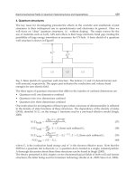
Introduction
The main tasks that face Engineers and Scientists that deal with fluid behavior in pipes can
be divided into two broad categories – the computation of flow rate and prediction of
pressure at some section of the pipe. Whether in computation of flow rate, or in pressure
transverse, the method employed is to solve the energy equation (Bernoulli equation for
19
Natural Gas436
liquid and Euler equation for compressible fluid), simultaneously with the equation of lost
head during fluid flow, the Colebrook (1938) friction factor equation for fluid flow in pipes
and the equation of continuity (conservation of mass / weight). For the case of a gas the
equation of state for gases is also included to account for the variation of gas volume with
pressure and temperature.
In the first part of this work, the Euler equation for the steady flow of any fluid in a pipe/
conduit is combined with the Darcy – Weisbach equation for the lost head during fluid flow
in pipes and the Colebrook friction factor equation. The combination yields a general
differential equation applicable to any compressible fluid; in a static column, or flowing
through a pipe. The pipe may be horizontal, inclined uphill or down hill.
The accuracy of the differential equation was ascertained by applying it to a problem of
uphill gas flow in a vertical well. The problem came from the book of Ikoku (1984), “Natural
Gas Production Engineering”. The classical fourth order Runge-Kutta method was first of all
programmed in FORTRAN to solve the differential equation. By use of the average
temperature and gas deviation factor method, Ikoku obtained the flowing bottom hole
pressure (P
w f
) as 2543 psia for the 5700 ft well. The Cullender and Smith (1956) method
that allows wide variation of temperature gave a P
w f
of 2544 psia. The computer program

obtaines the flowing bottom hole pressure (P
w f
) as 2544.8 psia. Ouyang and Aziz (1996)
developed another average temperature and deviation method for the calculation of flow
rate and pressure transverse in gas wells. The average temperature and gas deviation
formulas cannot be used directly to obtain pressure transverse in gas wells. The Cullender
and Smith method involves numerical integration and is long and tedious to use.
The next thing in this work was to use the Runge-Kutta method to generate formulas
suitable for the direct calculation of the pressure transverse in a static gas column, and in
uphill and downhill dipping pipes. The accuracy of the formula is tested by application to
two problems from the book of Ikoku. The first problem was prediction of static bottom hole
pressure (P w s). The new formula gives a P w s of 2640 psia for the 5790ft deep gas well.
Ikoku average pressure and gas deviation factor method gives the
P w s as 2639 psia, while the Cullender and Smith method gives the P w s as 2641 psia. The
second problem involves the calculation of flowing bottom hole pressure (P
w f
). The new
formula gives the P
w f
as 2545 psia while the average temperature and gas deviation factor
of Ikoku gives the P
w f
as 2543 psia. The Cullender and Smith method obtains a P
w f
of
2544 psia. The downhill formula was first tested by its application to a slight modification of
a problem from the book of Giles et al.(2009). There was a close agreement between exit
pressure calculated by the formula and that from the text book. The formula is also used to
calculate bottom hole pressure in a gas injection well.
The direct pressure transverse formulas developed in this work are also combined wit the

Reynolds number and the Colebrook friction factor equation to provide formulas for the
direct calculation of the gas volumetric rate in uphill and down hill dipping pipes.


A differntial equation for static behaviour of a compressible
fluid and its flow in pipes
The Euler equation is generally accepted for the flow of a compressible fluid in a pipe. The
equation from Giles et al. (2009) is:


l
dp
vdv

d sin dh 0
g

   

 (1)

In equation (1), the plus sign (+) before d  sin

corresponds to the upward direction of the
positive z coordinate and the minus sign (-) to the downward direction of the positive z
coordinate.
The generally accepted equation for the loss of head in a pipe transporting a fluid is that of
Darcy-Weisbach. The equation is:

2

L
f L v
H
2gd

(2)


The equation of continuity for compressible flow in a pipe is:

W =


A
(3)

Taking the first derivation of equation (3) and solving simultaneously with equation (1) and
(2) we have after some simplifications,


2
2
2
2 2
f W
sin .
2 A dg
dp

d

d
W
1
dp
A g











 














(4)

All equations used to derive equation (4) are generally accepted equations No limiting
assumptions were made during the combination of these equations. Thus, equation (4) is a
general differential equation that governs static behavior compressible fluid flow in a pipe.
The compressible fluid can be a liquid of constant compressibility, gas or combination of gas
and liquid (multiphase flow).
By noting that the compressibility of a fluid (C
f
) is:


f
d
1
C
dp



(5)

Equation (4) can be written as:
Static behaviour of natural gas and its ow in pipes 437
liquid and Euler equation for compressible fluid), simultaneously with the equation of lost
head during fluid flow, the Colebrook (1938) friction factor equation for fluid flow in pipes
and the equation of continuity (conservation of mass / weight). For the case of a gas the
equation of state for gases is also included to account for the variation of gas volume with
pressure and temperature.
In the first part of this work, the Euler equation for the steady flow of any fluid in a pipe/

conduit is combined with the Darcy – Weisbach equation for the lost head during fluid flow
in pipes and the Colebrook friction factor equation. The combination yields a general
differential equation applicable to any compressible fluid; in a static column, or flowing
through a pipe. The pipe may be horizontal, inclined uphill or down hill.
The accuracy of the differential equation was ascertained by applying it to a problem of
uphill gas flow in a vertical well. The problem came from the book of Ikoku (1984), “Natural
Gas Production Engineering”. The classical fourth order Runge-Kutta method was first of all
programmed in FORTRAN to solve the differential equation. By use of the average
temperature and gas deviation factor method, Ikoku obtained the flowing bottom hole
pressure (P
w f
) as 2543 psia for the 5700 ft well. The Cullender and Smith (1956) method
that allows wide variation of temperature gave a P
w f
of 2544 psia. The computer program
obtaines the flowing bottom hole pressure (P
w f
) as 2544.8 psia. Ouyang and Aziz (1996)
developed another average temperature and deviation method for the calculation of flow
rate and pressure transverse in gas wells. The average temperature and gas deviation
formulas cannot be used directly to obtain pressure transverse in gas wells. The Cullender
and Smith method involves numerical integration and is long and tedious to use.
The next thing in this work was to use the Runge-Kutta method to generate formulas
suitable for the direct calculation of the pressure transverse in a static gas column, and in
uphill and downhill dipping pipes. The accuracy of the formula is tested by application to
two problems from the book of Ikoku. The first problem was prediction of static bottom hole
pressure (P w s). The new formula gives a P w s of 2640 psia for the 5790ft deep gas well.
Ikoku average pressure and gas deviation factor method gives the
P w s as 2639 psia, while the Cullender and Smith method gives the P w s as 2641 psia. The
second problem involves the calculation of flowing bottom hole pressure (P

w f
). The new
formula gives the P
w f
as 2545 psia while the average temperature and gas deviation factor
of Ikoku gives the P
w f
as 2543 psia. The Cullender and Smith method obtains a P
w f
of
2544 psia. The downhill formula was first tested by its application to a slight modification of
a problem from the book of Giles et al.(2009). There was a close agreement between exit
pressure calculated by the formula and that from the text book. The formula is also used to
calculate bottom hole pressure in a gas injection well.
The direct pressure transverse formulas developed in this work are also combined wit the
Reynolds number and the Colebrook friction factor equation to provide formulas for the
direct calculation of the gas volumetric rate in uphill and down hill dipping pipes.


A differntial equation for static behaviour of a compressible
fluid and its flow in pipes
The Euler equation is generally accepted for the flow of a compressible fluid in a pipe. The
equation from Giles et al. (2009) is:


l
dp
vdv

d sin dh 0

g
    

 (1)

In equation (1), the plus sign (+) before d  sin

corresponds to the upward direction of the
positive z coordinate and the minus sign (-) to the downward direction of the positive z
coordinate.
The generally accepted equation for the loss of head in a pipe transporting a fluid is that of
Darcy-Weisbach. The equation is:

2
L
f L v
H
2gd

(2)


The equation of continuity for compressible flow in a pipe is:

W =


A
(3)

Taking the first derivation of equation (3) and solving simultaneously with equation (1) and
(2) we have after some simplifications,


2
2
2
2 2
f W
sin .
2 A dg
dp

d
d
W
1
dp
A g
 
 
 

 
 
 
 


 


 
 


(4)

All equations used to derive equation (4) are generally accepted equations No limiting
assumptions were made during the combination of these equations. Thus, equation (4) is a
general differential equation that governs static behavior compressible fluid flow in a pipe.
The compressible fluid can be a liquid of constant compressibility, gas or combination of gas
and liquid (multiphase flow).
By noting that the compressibility of a fluid (C
f
) is:


f
d
1
C
dp



(5)

Equation (4) can be written as:
Natural Gas438

2
2
2
f
2
fW
sin
2 A dg
dp
d
W C
1
A g
 
 
 

 
 

 

 

 
 


(6)

Equation (6) can be simplified further for a gas.
Multiply through equation (6) by

, then


2
2
2
2
f
2
f W
sin
2g dg
dp
d
W C
1
A g
 
 
 


 


 
 


 

 
 


(7)

The equation of state for a non-ideal gas can be written as


p
zR

 

(8)

Substitution of equation (8) into equation (7) and using the fact that


2
2
2
2
2
2
f
2

pdp dp
1
, gives
d 2 d
2p sin
fW zR
zR
d g
dp
d
W zR C
1
g p

 
 

 

 
 
 
 
 


 

 
 

 


(9)
The cross-sectional area (A) of a pipe is


2
2 2 4
2
d d
4 16
 
 
  
 
 
 
(10)

Then equation (9) becomes:

2
2
5
2
2
f
4
2 sin

fW zR
1.621139
zR
d g
d
.
d
1.621139W zR C
1
g d


 








 









 




(11)

The denominator of equation (11) accounts for the effect of the change in kinetic energy
during fluid flow in pipes. The kinetic effect is small and can be neglected as pointed out by
previous researchers such as Ikoku (1984) and Uoyang and Aziz(1996). Where the kinetic
effect is to be evaluated, the compressibility of the gas (C
f
) can be calculated as follows:
For an ideal gas such as air,

.
p
1
C
f
 For a non ideal gas, C
f
=
p
z
zp 


11
.

Matter et al. (1975) and Ohirhian (2008) have proposed equations for the calculation of the
compressibility of hydrocarbon gases. For a sweet natural gas (natural gas that contains CO
2

as major contaminant), Ohirhian (2008) has expressed the compressibility of the real gas (C
f
)
as:
p
C
f


For Nigerian (sweet) natural gas K = 1.0328 when p is in psia
The denominator of equation (11) can then be written as

24
2
Pd g M
zRTKW
1 , where K = constant.
Then equation (11) can be written as

d
y
(A B
y
)
G

d
(1 )
y




(12)

where
2 2
2
5 4
1.621139fW zRT 2Msin KW zRT
y
p , A , B , G .
zRT
gd M gMd

   


The plus (+) sign in numerator of equation (12) is used for compressible uphill flow and the
negative sign (-) is used for the compressible downhill flow. In both cases the z coordinate is
taken positive upward. In equation (12) the pressure drop is y - y
21
, with y
1
> y
2

and
incremental length is l
2
– l
1.
Flow occurs from point (1) to point (2). Uphill flow of gas occurs
in gas transmission lines and flow from the foot of a gas well to the surface. The pressure at
Static behaviour of natural gas and its ow in pipes 439

2
2
2
f
2
fW
sin
2 A dg
dp
d
W C
1
A g













 

 

 
 


(6)

Equation (6) can be simplified further for a gas.
Multiply through equation (6) by

, then


2
2
2
2
f
2
f W
sin
2g dg
dp

d
W C
1
A g












 
 

 

 
 


(7)

The equation of state for a non-ideal gas can be written as

p
zR

 

(8)

Substitution of equation (8) into equation (7) and using the fact that


2
2
2
2
2
2
f
2
pdp dp
1
, gives
d 2 d
2p sin
fW zR
zR
d g
dp
d
W zR C
1

g p









 




 
 


 

 
 
 


(9)
The cross-sectional area (A) of a pipe is

2
2 2 4
2
d d
4 16
 
 
  
 
 
 
(10)

Then equation (9) becomes:

2
2
5
2
2
f
4
2 sin
fW zR
1.621139
zR
d g
d
.
d

1.621139W zR C
1
g d
 
 

 





 
 

 

 
 
 


(11)

The denominator of equation (11) accounts for the effect of the change in kinetic energy
during fluid flow in pipes. The kinetic effect is small and can be neglected as pointed out by
previous researchers such as Ikoku (1984) and Uoyang and Aziz(1996). Where the kinetic
effect is to be evaluated, the compressibility of the gas (C
f
) can be calculated as follows:

For an ideal gas such as air,

.
p
1
C
f
 For a non ideal gas, C
f
=
p
z
zp 


11
.

Matter et al. (1975) and Ohirhian (2008) have proposed equations for the calculation of the
compressibility of hydrocarbon gases. For a sweet natural gas (natural gas that contains CO
2

as major contaminant), Ohirhian (2008) has expressed the compressibility of the real gas (C
f
)
as:
p
C
f



For Nigerian (sweet) natural gas K = 1.0328 when p is in psia
The denominator of equation (11) can then be written as

24
2
Pd g M
zRTKW
1 , where K = constant.
Then equation (11) can be written as

dy (A By)
G
d
(1 )
y




(12)

where
2 2
2
5 4
1.621139fW zRT 2Msin KW zRT
y
p , A , B , G .
zRT

gd M gMd

   


The plus (+) sign in numerator of equation (12) is used for compressible uphill flow and the
negative sign (-) is used for the compressible downhill flow. In both cases the z coordinate is
taken positive upward. In equation (12) the pressure drop is y - y
21
, with y
1
> y
2
and
incremental length is l
2
– l
1.
Flow occurs from point (1) to point (2). Uphill flow of gas occurs
in gas transmission lines and flow from the foot of a gas well to the surface. The pressure at
Natural Gas440
the surface is usually known. Downhill flow of gas occurs in gas injection wells and gas
transmission lines.
We shall illustrate the solution to the compressible flow equation by taking a problem
involving an uphill flow of gas in a vertical gas well.

Computation of the variables in the gas differential equation
We need to discuss the computation of the variables that occur in the differential equation
for gas before finding a suitable solution to it The gas deviation factor (z) can be obtained
from the chart of Standing and Katz (1942). The Standing and Katz chart has been curve

fitted by many researchers. The version that was used in this section of the work that of
Gopal(1977). The dimensionless friction factor in the compressible flow equation is a
function of relative roughness (

/ d) and the Reynolds number (R
N
). The Reynolds
number is defined as:

N
Wd
vd
R
A
g

 
 
(13)

The Reynolds number can also be written in terms of the gas volumetric flow rate. Then

W =

b
Q
b

Since the specific weight at base condition is:

p M 28.97G p
g
b b

b
z T R z T R
b b b b
  
(14)

The Reynolds number can be written as:


g
b b
N
b b
g
36.88575G P Q
R
Rgd z T


(15)

By use of a base pressure (p
b
) = 14.7psia, base temperature (T
b

) = 520
o
R and R = 1545

R
N
=
b g
g
20071Q G
d
(16)

Where d is expressed in inches, Q
b
= MMSCF / Day and
g

is in centipoises.
Ohirhian and Abu (2008) have presented a formula for the calculation of the viscosity of
natural gas. The natural gas can contain impurities of CO
2
and H
2
S. The formula is:


2
2
g

0.0109388 0.0088234xx 0.00757210xx

1.0 1.3633077xx 0.0461989xx
 
 
 
(17)
Where
xx =
0.0059723p
T
z 16.393443
p
 

 
 


In equation (17)
g

is expressed in centipoises(c
p
) , p in (psia) and Tin (
o
R)
The generally accepted equation for the calculation of the dimensionless friction factor (f) is
that of Colebrook (1938). The equation is:

N
1 2.51
2log
3.7d
f R f
 

  
 
 
 
(18)

The equation is non-linear and requires iterative solution. Several researchers have
proposed equations for the direct calculation of f. The equation used in this work is that
proposed by Ohirhian (2005). The equation is


 
 
1
2
f 2 log a 2b log a bx



   



(19)

Where
2.51
a , b .
3.7d R


 

x
1
=
 
N N
1.14lo
g
0.30558 0.57lo
g
R 0.01772lo
g
R 1.0693
d

 
   
 
 

After evaluating the variables in the gas differential equation, a suitable numerical scheme

can be used to it.

Solution to the gas differential equation for direct calculation of pressure transverse in
static and uphill gas flow in pipes.


The classical fourth order Range Kutta method that allows large increment in the
independent variable when used to solve a differential equation is used in this work. The
solution by use of the Runge-Kutta method allows direct calculation of pressure transverse
The Runge-Kutta approximate solution to the differential equation
Static behaviour of natural gas and its ow in pipes 441
the surface is usually known. Downhill flow of gas occurs in gas injection wells and gas
transmission lines.
We shall illustrate the solution to the compressible flow equation by taking a problem
involving an uphill flow of gas in a vertical gas well.

Computation of the variables in the gas differential equation
We need to discuss the computation of the variables that occur in the differential equation
for gas before finding a suitable solution to it The gas deviation factor (z) can be obtained
from the chart of Standing and Katz (1942). The Standing and Katz chart has been curve
fitted by many researchers. The version that was used in this section of the work that of
Gopal(1977). The dimensionless friction factor in the compressible flow equation is a
function of relative roughness (

/ d) and the Reynolds number (R
N
). The Reynolds
number is defined as:

N

Wd
vd
R
A
g

 


(13)

The Reynolds number can also be written in terms of the gas volumetric flow rate. Then

W =

b
Q
b

Since the specific weight at base condition is:


p M 28.97G p
g
b b

b
z T R z T R
b b b b
  

(14)

The Reynolds number can be written as:


g
b b
N
b b
g
36.88575G P Q
R
Rgd z T


(15)

By use of a base pressure (p
b
) = 14.7psia, base temperature (T
b
) = 520
o
R and R = 1545

R
N
=
b
g

g
20071Q G
d
(16)

Where d is expressed in inches, Q
b
= MMSCF / Day and
g

is in centipoises.
Ohirhian and Abu (2008) have presented a formula for the calculation of the viscosity of
natural gas. The natural gas can contain impurities of CO
2
and H
2
S. The formula is:


2
2
g
0.0109388 0.0088234xx 0.00757210xx

1.0 1.3633077xx 0.0461989xx
 
 
 
(17)
Where

xx =
0.0059723p
T
z 16.393443
p
 

 
 


In equation (17)
g
 is expressed in centipoises(c
p
) , p in (psia) and Tin (
o
R)
The generally accepted equation for the calculation of the dimensionless friction factor (f) is
that of Colebrook (1938). The equation is:


N
1 2.51
2log
3.7d
f R f
 

  

 
 
 
(18)

The equation is non-linear and requires iterative solution. Several researchers have
proposed equations for the direct calculation of f. The equation used in this work is that
proposed by Ohirhian (2005). The equation is


 
 
1
2
f 2 log a 2b log a bx

 
   
 
(19)

Where
2.51
a , b .
3.7d R


 

x

1
=
 
N N
1.14lo
g
0.30558 0.57lo
g
R 0.01772lo
g
R 1.0693
d

 
   
 
 

After evaluating the variables in the gas differential equation, a suitable numerical scheme
can be used to it.

Solution to the gas differential equation for direct calculation of pressure transverse in
static and uphill gas flow in pipes.


The classical fourth order Range Kutta method that allows large increment in the
independent variable when used to solve a differential equation is used in this work. The
solution by use of the Runge-Kutta method allows direct calculation of pressure transverse
The Runge-Kutta approximate solution to the differential equation
Natural Gas442

n
o o
o 1 2 3 4
dy
f(x,y) at x x
dx
given that y y when x x is
1
y y (k 2(k k ) k )
6
where
 
 
    


1 o o
2 o 1
1 1
2 2
k Hf(x ,y )
k Hf(x H,y k )

  

3 o o 1
4 o 3
n o
1 1
2 2

k Hf(x H,
y
k )
k Hf(x H, y k )
x x
H
n
n number of applications
  
  





The Runge-Kutta algorithm can obtain an accurate solution with a large value of H. The
Runge-Kutta Algorithm can solve equation (6) or (12). The test problem used in this work is
from the book of Ikoku (1984), “Natural Gas Production Engineering”. Ikoku has solved this
problem with some of the available methods in the literature.

Example 1
Calculate the sand face pressure (p
wf
) of a flowing gas well from the following surface
measurements.
Flow rate (Q) = 5.153 MMSCF / Day
Tubing internal diameter (d) = 1.9956in
Gas gravity (G g) = 0.6
Depth = 5790ft (bottom of casing)
Temperature at foot of tubing (T

w f
) = 160
o
F
Surface temperature (T
s f
) = 83
o
F
Tubing head pressure (p
t f
) = 2122 psia
Absolute roughness of tubing (

) = 0.0006 in
Length of tubing (l) = 5700ft (well is vertical)
Solution
When length (

) is zero, p = 2122 psia
That is (x
o
, y
o
) = (0, 2122)
By use of 1 step Runge-Kutta.
H =
.ft5700
1
05700




(20)
(21)
The Runge-Kutta algorithm is programmed in Fortran 77 and used to solve this problem.
The program is also used to study the size of depth(length ) increment needed to obtain an
accurate solution by use of the Runge-Kutta method. The first output shows result for one-
step Runge-Kutta (Depth increment = 5700ft). The program obtaines 2544.823 psia as the
flowing bottom hole pressure (P
w f
).

TUBING HEAD PRESSURE = 2122.0000000 PSIA
SURFACE TEMPERATURE = 543.0000000 DEGREE RANKINE
TEMPERATURE AT TOTAL DEPTH = 620.0000000 DEGREE RANKINE
GAS GRAVITY = 6.000000E-001
GAS FLOW RATE = 5.1530000 MMSCFD
DEPTH AT SURFACE = .0000000 FT
TOTAL DEPTH = 5700.0000000 FT
INTERNAL TUBING DIAMETER = 1.9956000 INCHES
ROUGHNESS OF TUBING = 6.000000E-004 INCHES
INCREMENTAL DEPTH = 5700.0000000 FT

PRESSURE PSIA DEPTH FT

2122.000 .000
2544.823 5700.000

To check the accuracy of the Runge-Kutta algorithm for the depth increment of 5700 ft

another run is made with a smaller length increment of 1000 ft. The output gives a p
wf
of
2544.823 psia. as it is with a depth increment of 5700 ft. This confirmes that the Runge-
Kutta solution can be accurate for a length increment of 5700 ft.

TUBING HEAD PRESSURE = 2122.0000000 PSIA
SURFACE TEMPERATURE = 543.0000000 DEGREE RANKINE
TEMPERATURE AT TOTAL DEPTH = 620.0000000 DEGREE RANKINE
GAS GRAVITY = 6.000000E-001
GAS FLOW RATE = 5.1530000 MMSCFD
DEPTH AT SURFACE = .0000000 FT
TOTAL DEPTH = 5700.0000000 FT
INTERNAL TUBING DIAMETER = 1.9956000 INCHES
ROUGHNESS OF TUBING = 6.000000E-004 INCHES
INCREMENTAL DEPTH = 1000.0000000 FT

PRESSURE PSIA DEPTH FT
2122.000 .000
2206.614 1140.000
2291.203 2280.000
2375.767 3420.000
2460.306 4560.000
2544.823 5700.000
Static behaviour of natural gas and its ow in pipes 443
n
o o
o 1 2 3 4
dy
f(x,y) at x x

dx
g
iven that
y y
when x x is
1
y y (k 2(k k ) k )
6
where
 
 
    


1 o o
2 o 1
1 1
2 2
k Hf(x ,y )
k Hf(x H,
y
k )

  

3 o o 1
4 o 3
n o
1 1
2 2

k Hf(x H,
y
k )
k Hf(x H, y k )
x x
H
n
n number of applications
  
  





The Runge-Kutta algorithm can obtain an accurate solution with a large value of H. The
Runge-Kutta Algorithm can solve equation (6) or (12). The test problem used in this work is
from the book of Ikoku (1984), “Natural Gas Production Engineering”. Ikoku has solved this
problem with some of the available methods in the literature.

Example 1
Calculate the sand face pressure (p
wf
) of a flowing gas well from the following surface
measurements.
Flow rate (Q) = 5.153 MMSCF / Day
Tubing internal diameter (d) = 1.9956in
Gas gravity (G g) = 0.6
Depth = 5790ft (bottom of casing)
Temperature at foot of tubing (T

w f
) = 160
o
F
Surface temperature (T
s f
) = 83
o
F
Tubing head pressure (p
t f
) = 2122 psia
Absolute roughness of tubing (

) = 0.0006 in
Length of tubing (l) = 5700ft (well is vertical)
Solution
When length (

) is zero, p = 2122 psia
That is (x
o
, y
o
) = (0, 2122)
By use of 1 step Runge-Kutta.
H =
.ft5700
1
05700




(20)
(21)
The Runge-Kutta algorithm is programmed in Fortran 77 and used to solve this problem.
The program is also used to study the size of depth(length ) increment needed to obtain an
accurate solution by use of the Runge-Kutta method. The first output shows result for one-
step Runge-Kutta (Depth increment = 5700ft). The program obtaines 2544.823 psia as the
flowing bottom hole pressure (P
w f
).

TUBING HEAD PRESSURE = 2122.0000000 PSIA
SURFACE TEMPERATURE = 543.0000000 DEGREE RANKINE
TEMPERATURE AT TOTAL DEPTH = 620.0000000 DEGREE RANKINE
GAS GRAVITY = 6.000000E-001
GAS FLOW RATE = 5.1530000 MMSCFD
DEPTH AT SURFACE = .0000000 FT
TOTAL DEPTH = 5700.0000000 FT
INTERNAL TUBING DIAMETER = 1.9956000 INCHES
ROUGHNESS OF TUBING = 6.000000E-004 INCHES
INCREMENTAL DEPTH = 5700.0000000 FT

PRESSURE PSIA DEPTH FT

2122.000 .000
2544.823 5700.000

To check the accuracy of the Runge-Kutta algorithm for the depth increment of 5700 ft

another run is made with a smaller length increment of 1000 ft. The output gives a p
wf
of
2544.823 psia. as it is with a depth increment of 5700 ft. This confirmes that the Runge-
Kutta solution can be accurate for a length increment of 5700 ft.

TUBING HEAD PRESSURE = 2122.0000000 PSIA
SURFACE TEMPERATURE = 543.0000000 DEGREE RANKINE
TEMPERATURE AT TOTAL DEPTH = 620.0000000 DEGREE RANKINE
GAS GRAVITY = 6.000000E-001
GAS FLOW RATE = 5.1530000 MMSCFD
DEPTH AT SURFACE = .0000000 FT
TOTAL DEPTH = 5700.0000000 FT
INTERNAL TUBING DIAMETER = 1.9956000 INCHES
ROUGHNESS OF TUBING = 6.000000E-004 INCHES
INCREMENTAL DEPTH = 1000.0000000 FT

PRESSURE PSIA DEPTH FT
2122.000 .000
2206.614 1140.000
2291.203 2280.000
2375.767 3420.000
2460.306 4560.000
2544.823 5700.000
Natural Gas444
In order to determine the maximum length of pipe (depth) for which the computed P
w f

can be considered as accurate, the depth of the test well is arbitrarily increased to 10,000ft
and the program run with one step (length increment = 10,000ft). The program produces the

P
w f
as 2861.060 psia

TUBING HEAD PRESSURE = 2122.0000000 PSIA
SURFACE TEMPERATURE = 543.0000000 DEGREE RANKINE
TEMPERATURE AT TOTAL DEPTH = 687.0000000 DEGREE RANKINE
GAS GRAVITY = 6.000000E-001
GAS FLOW RATE = 5.1530000 MMSCFD
DEPTH AT SURFACE = .0000000 FT
TOTAL DEPTH = 10000.0000000 FT
INTERNAL TUBING DIAMETER = 1.9956000 INCHES
ROUGHNESS OF TUBING = 6.000000E-004 INCHES
INCREMENTAL DEPTH = 10000.0000000 FT

PRESSURE PSIA DEPTH FT

2122.000 .000
2861.060 10000.000

Next the total depth of 10000ft is subdivided into ten steps (length increment = 1,000ft). The
program gives the P
w f
as 2861.057 psia for the length increment of 1000ft.

TUBING HEAD PRESSURE = 2122.0000000 PSIA
SURFACE TEMPERATURE = 543.0000000 DEGREE RANKINE
TEMPERATURE AT TOTAL DEPTH = 687.0000000 DEGREE RANKINE
GAS GRAVITY = 6.000000E-001
GAS FLOW RATE = 5.1530000 MMSCFD

DEPTH AT SURFACE = .0000000 FT
TOTAL DEPTH = 10000.0000000 FT
INTERNAL TUBING DIAMETER = 1.9956000 INCHES
ROUGHNESS OF TUBING = 6.000000E-004 INCHES
INCREMENTAL DEPTH = 1000.0000000 FT

PRESSURE PSIA DEPTH FT
2122.000 .000
2197.863 1000.000
2273.246 2000.000
2348.165 3000.000
2422.638 4000.000
2496.680 5000.000
2570.311 6000.000
2643.547 7000.000
2716.406 8000.000
2788.903 9000.000
2861.057 10000.000
The computed values of P
w f
for the depth increment of 10,000ft and 1000ft differ only in
the third decimal place. This suggests that the depth increment for the Range - Kutta
solution to the differential equation generated in this work could be a large as 10,000ft. By
neglecting the denominator of equation (6) that accounts for the kinetic effect, the
result can be compared with Ikoku’s average temperature and gas deviation method that
uses an average value of the gas deviation factor (z) and negligible kinetic effects. In the
program z is allowed to vary with pressure and temperature. The temperature in the
program also varies with depth (length of tubing) as
T = GTG


current length + T
s f,
where,
s
wf f
(T T )
GTG
Total Depth



The program obtains the P
w f
as

2544.737 psia when the kinetic effect is ignored. The
output is as follows:


TUBING HEAD PRESSURE = 2122.0000000 PSIA
SURFACE TEMPERATURE = 543.0000000 DEGREE RANKINE
TEMPERATURE AT TOTAL DEPTH = 620.0000000 DEGREE RANKINE
GAS GRAVITY = 6.000000E-001
GAS FLOW RATE = 5.1530000 MMSCFD
DEPTH AT SURFACE = .0000000 FT
TOTAL DEPTH = 5700.0000000 FT
INTERNAL TUBING DIAMETER = 1.9956000 INCHES
ROUGHNESS OF TUBING = 6.000000E-004 INCHES
INCREMENTAL DEPTH = 5700.0000000 FT

PRESSURE PSIA DEPTH FT

2122.000 .000
2544.737 5700.000

Comparing the P
w f
of 2544.737 psia with the P
w f
of 2544.823 psia when the kinetic effect is
considered, the kinetic contribution to the pressure drop is 2544.823 psia – 2544.737psia =
0.086 psia.The kinetic effect during calculation of pressure transverse in uphill dipping pipes
is small and can be neglected as pointed out by previous researchers such as Ikoku (1984)
and Uoyang and Aziz(1996)
Ikoku obtained 2543 psia by use of the the average temperature and gas deviation method.
The average temperature and gas deviation method goes through trial and error calculations
in order to obtain an accurate solution. Ikoku also used the Cullendar and Smith method to
solve the problem under consideration. The Cullendar and Smith method does not consider
the kinetic effect but allows a wide variation of the temperature. The Cullendar and Smith
method involves the use of Simpson rule to carry out an integration of a cumbersome
function. The solution to the given problem by the Cullendar and Smith method is p
w f
=
2544 psia.
If we neglect the denominator of equation (12), then the differential equation for pressure
transverse in a flowing gas well becomes
Static behaviour of natural gas and its ow in pipes 445
In order to determine the maximum length of pipe (depth) for which the computed P
w f

can be considered as accurate, the depth of the test well is arbitrarily increased to 10,000ft
and the program run with one step (length increment = 10,000ft). The program produces the
P
w f
as 2861.060 psia

TUBING HEAD PRESSURE = 2122.0000000 PSIA
SURFACE TEMPERATURE = 543.0000000 DEGREE RANKINE
TEMPERATURE AT TOTAL DEPTH = 687.0000000 DEGREE RANKINE
GAS GRAVITY = 6.000000E-001
GAS FLOW RATE = 5.1530000 MMSCFD
DEPTH AT SURFACE = .0000000 FT
TOTAL DEPTH = 10000.0000000 FT
INTERNAL TUBING DIAMETER = 1.9956000 INCHES
ROUGHNESS OF TUBING = 6.000000E-004 INCHES
INCREMENTAL DEPTH = 10000.0000000 FT

PRESSURE PSIA DEPTH FT

2122.000 .000
2861.060 10000.000

Next the total depth of 10000ft is subdivided into ten steps (length increment = 1,000ft). The
program gives the P
w f
as 2861.057 psia for the length increment of 1000ft.

TUBING HEAD PRESSURE = 2122.0000000 PSIA
SURFACE TEMPERATURE = 543.0000000 DEGREE RANKINE
TEMPERATURE AT TOTAL DEPTH = 687.0000000 DEGREE RANKINE

GAS GRAVITY = 6.000000E-001
GAS FLOW RATE = 5.1530000 MMSCFD
DEPTH AT SURFACE = .0000000 FT
TOTAL DEPTH = 10000.0000000 FT
INTERNAL TUBING DIAMETER = 1.9956000 INCHES
ROUGHNESS OF TUBING = 6.000000E-004 INCHES
INCREMENTAL DEPTH = 1000.0000000 FT

PRESSURE PSIA DEPTH FT
2122.000 .000
2197.863 1000.000
2273.246 2000.000
2348.165 3000.000
2422.638 4000.000
2496.680 5000.000
2570.311 6000.000
2643.547 7000.000
2716.406 8000.000
2788.903 9000.000
2861.057 10000.000
The computed values of P
w f
for the depth increment of 10,000ft and 1000ft differ only in
the third decimal place. This suggests that the depth increment for the Range - Kutta
solution to the differential equation generated in this work could be a large as 10,000ft. By
neglecting the denominator of equation (6) that accounts for the kinetic effect, the
result can be compared with Ikoku’s average temperature and gas deviation method that
uses an average value of the gas deviation factor (z) and negligible kinetic effects. In the
program z is allowed to vary with pressure and temperature. The temperature in the
program also varies with depth (length of tubing) as

T = GTG

current length + T
s f,
where,
s
wf f
(T T )
GTG
Total Depth



The program obtains the P
w f
as

2544.737 psia when the kinetic effect is ignored. The
output is as follows:


TUBING HEAD PRESSURE = 2122.0000000 PSIA
SURFACE TEMPERATURE = 543.0000000 DEGREE RANKINE
TEMPERATURE AT TOTAL DEPTH = 620.0000000 DEGREE RANKINE
GAS GRAVITY = 6.000000E-001
GAS FLOW RATE = 5.1530000 MMSCFD
DEPTH AT SURFACE = .0000000 FT
TOTAL DEPTH = 5700.0000000 FT
INTERNAL TUBING DIAMETER = 1.9956000 INCHES
ROUGHNESS OF TUBING = 6.000000E-004 INCHES

INCREMENTAL DEPTH = 5700.0000000 FT

PRESSURE PSIA DEPTH FT

2122.000 .000
2544.737 5700.000

Comparing the P
w f
of 2544.737 psia with the P
w f
of 2544.823 psia when the kinetic effect is
considered, the kinetic contribution to the pressure drop is 2544.823 psia – 2544.737psia =
0.086 psia.The kinetic effect during calculation of pressure transverse in uphill dipping pipes
is small and can be neglected as pointed out by previous researchers such as Ikoku (1984)
and Uoyang and Aziz(1996)
Ikoku obtained 2543 psia by use of the the average temperature and gas deviation method.
The average temperature and gas deviation method goes through trial and error calculations
in order to obtain an accurate solution. Ikoku also used the Cullendar and Smith method to
solve the problem under consideration. The Cullendar and Smith method does not consider
the kinetic effect but allows a wide variation of the temperature. The Cullendar and Smith
method involves the use of Simpson rule to carry out an integration of a cumbersome
function. The solution to the given problem by the Cullendar and Smith method is p
w f
=
2544 psia.
If we neglect the denominator of equation (12), then the differential equation for pressure
transverse in a flowing gas well becomes
Natural Gas446

2
5
g
dy
A By
dl
where
1.621139fW zRT
A
gd M
2 28.79G sin
2Msin
B
zRT RTz
 

 

 


The equation is valid in any consistent set of units. If we assume that the pressure and
temperature in the tubing are held constant from the mid section of the pipe to the foot of
the tubing, the Runge-Kutta method can be used to obtain the pressure transverse in the
tubing as follows.

2
b
5
2

2
b
b
4
b
46.9643686GgQ fzRT 59.940Gg Sin y
zRT
dy gd
d
46.9643686KzGgQ
p
T
1
T y
gRd



 
 

 
 
 
 

(25)

The weight flow rate (W) in equation (12) is related to Q
b

(the volumetric rate measurement
at a base pressure (P
b
) and a base temperature (T
b
)) in equation (25) by:

W =

b
Q
b
(26)

Equation (25) is a general differential equation that governs pressure transverse in a gas
pipe that conveys gas uphill. When the angle of inclination (

) is zero, sin

is zero and the
differential equation reduces to that of a static gas column. The differential equation (25) is
valid in any consistent set of units. The constant K = 1.0328 for Nigerian Natural Gas when
the unit of pressure is psia.
The classical 4
th
order Runge Kutta alogarithm can be used to provide a formula that serves
as a general solution to the differential equation (25). To achieve this, the temperature and
gas deviation factors are held constant at some average value, starting from the mid section
of the pipe to the inlet end of the pipe. The solution to equation (25) by the Runge Katta
algorithm can be written as:

2
1 2
p p
y
. 
(27)



Where
(22)
(23)
(24)
     
2
2 3 2 3 2
2
p
aa u
y 1 x 0.5x 0.36x 4.96x 1.48x 0.72x 4.96 1.96x 0.72x
6 6 6
         

2 2
g b 2 2 2 g 2
5
2 z
46.9643686G Q f z RT 57.94G sin

aa L
z R
gd
 

 
 
 

 

2
g b 2 av av
5
g
av av
46.9643686G Q f z L
u
gd
57.940G sin L
x
z T R





When Q
b
= 0, equation (27) reduces to the formula for pressure transverse in a static gas

column.
In equation (27), the component
k
4
in the Runge Kutta method given by k
4
=
H f(x
o
+ H, y + k
3
) was given some weighting to compensate for the fact that the
temperature and gas deviation factor vary between the mid section and the inlet end of the
pipe.
Equation (27) can be converted to oil field units. In oil field units in which L is in feet, R =
1545, temperature is in
o
R, g = 32.2 ft/sec
2
, diameter (d) is in inches, pressure (p) is in pound
per square inch (psia), flow rate (Q
b
) is in MMSCF / Day, P
b
= 14.7 psia and T
b
= 520
o
R.,the
variables aa, u and x that occur in equation (25) can be written as:

5
2
g
av av
2
b
25.130920G Q f z T L
u
d



g
av av
G L sin
x 0.03749
z T

 


The following steps are taken in order to use equation (27) to solve a problem.
1.
Evaluate the gas deviation factor at a given pressure and temperature. When
equation (27) is used to calculate pressure transverse in a gas well, the given
pressure and temperature are the surface temperature and gas exit pressure (tubing
head pressure).
2.
Evaluate the viscosity of the gas at surface condition. This step is only necessary

when calculating pressure transverse in a flowing gas well. It is omitted when
static pressure transverse is calculated.
3.
Evaluate the Reynolds number and dimensionless friction factor by use of surface
properties. This step is also omitted when considering a static gas column.
4.
Evaluate the coefficient aa in the formula. This coefficient depends only on surface
properties.
Static behaviour of natural gas and its ow in pipes 447

2
5
g
dy
A By
dl
where
1.621139fW zRT
A
gd M
2 28.79G sin
2Msin
B
zRT RTz
 




 

The equation is valid in any consistent set of units. If we assume that the pressure and
temperature in the tubing are held constant from the mid section of the pipe to the foot of
the tubing, the Runge-Kutta method can be used to obtain the pressure transverse in the
tubing as follows.

2
b
5
2
2
b
b
4
b
46.9643686G
g
Q fzRT 59.940G
g
Sin
y
zRT
dy gd
d
46.9643686KzGgQ
p
T
1
T y

gRd



 
 

 
 
 
 

(25)

The weight flow rate (W) in equation (12) is related to Q
b
(the volumetric rate measurement
at a base pressure (P
b
) and a base temperature (T
b
)) in equation (25) by:

W =

b
Q
b
(26)

Equation (25) is a general differential equation that governs pressure transverse in a gas
pipe that conveys gas uphill. When the angle of inclination (

) is zero, sin

is zero and the
differential equation reduces to that of a static gas column. The differential equation (25) is
valid in any consistent set of units. The constant K = 1.0328 for Nigerian Natural Gas when
the unit of pressure is psia.
The classical 4
th
order Runge Kutta alogarithm can be used to provide a formula that serves
as a general solution to the differential equation (25). To achieve this, the temperature and
gas deviation factors are held constant at some average value, starting from the mid section
of the pipe to the inlet end of the pipe. The solution to equation (25) by the Runge Katta
algorithm can be written as:


2
1 2
p p
y
.


(27)



Where

(22)
(23)
(24)
     
2
2 3 2 3 2
2
p
aa u
y 1 x 0.5x 0.36x 4.96x 1.48x 0.72x 4.96 1.96x 0.72x
6 6 6
         

2 2
g b 2 2 2 g 2
5
2 z
46.9643686G Q f z RT 57.94G sin
aa L
z R
gd
 

 
 
 

 

2

g b 2 av av
5
g
av av
46.9643686G Q f z L
u
gd
57.940G sin L
x
z T R





When Q
b
= 0, equation (27) reduces to the formula for pressure transverse in a static gas
column.
In equation (27), the component
k
4
in the Runge Kutta method given by k
4
=
H f(x
o
+ H, y + k
3
) was given some weighting to compensate for the fact that the

temperature and gas deviation factor vary between the mid section and the inlet end of the
pipe.
Equation (27) can be converted to oil field units. In oil field units in which L is in feet, R =
1545, temperature is in
o
R, g = 32.2 ft/sec
2
, diameter (d) is in inches, pressure (p) is in pound
per square inch (psia), flow rate (Q
b
) is in MMSCF / Day, P
b
= 14.7 psia and T
b
= 520
o
R.,the
variables aa, u and x that occur in equation (25) can be written as:

5
2
g
av av
2
b
25.130920G Q f z T L
u
d


g
av av
G L sin
x 0.03749
z T

 


The following steps are taken in order to use equation (27) to solve a problem.
1.
Evaluate the gas deviation factor at a given pressure and temperature. When
equation (27) is used to calculate pressure transverse in a gas well, the given
pressure and temperature are the surface temperature and gas exit pressure (tubing
head pressure).
2.
Evaluate the viscosity of the gas at surface condition. This step is only necessary
when calculating pressure transverse in a flowing gas well. It is omitted when
static pressure transverse is calculated.
3.
Evaluate the Reynolds number and dimensionless friction factor by use of surface
properties. This step is also omitted when considering a static gas column.
4.
Evaluate the coefficient aa in the formula. This coefficient depends only on surface
properties.
Natural Gas448
5. Evaluate the average pressure (p
a v
) and average temperature (T

a v
).
6.
Evaluate the average gas deviation factor.(z
a v
)
7.
Evaluate the coefficients x and u in the formula. Note that u = 0 when Q
b
= 0.
8.
Evaluate y in the formula.
9.
Evaluate the pressure
1
p . In a flowing gas well,
1
p is the flowing bottom hole
pressure. In a static column, it is the static bottom hole pressure.

Equation (27) is tested by using it to solve two problems from the book of Ikoku(1984),
“Natural Gas Production Engineering”. The first problem involves calculation of the static
bottom hole in a gas well. The second involves the calculation of the flowing bottom hole
pressure of a gas well.

Example 2
Calculate the static bottom hole pressure of a gas well having a depth of 5790 ft. The gas
gravity is 0.6 and the pressure at the well head is 2300 psia. The surface temperature is 83
o
F

and the average flowing temperature is 117
o
F.
Solution
Following the steps that were listed for the solution to a problem by use of equation (27) we
have:
1. Evaluation of z – factor.
The standing equation for P
c
and T
c
are:
P
c
(psia) = 677.0 + 15.0 G
g
– 37.5 G
g
2

T
c
(
o
R) = 168.0 + 325.0 G
g
– 12.5 G
g
2

Substitution of G
g
= 0.6 gives, P
c
= 672.5 psia and T
c
= 358.5
o
R. Then P
r
= 2300/672.5 = 3.42
and T
r
= 543/358.5 = 1.52
The Standing and Katz chart gives z
2
= 0.78.
Steps 2 and 3 omitted in the static case.

4.
2 2
g b 2 2 g 2
5
2 2
25.13092G Q fz T 0.037417G p sin
aa L
z T
d
 


 
 
 
 

Here, G
g
= 0.6, Q
b
= 0.0,
2
z = 0.78, d = 1.9956 inches,
2
p = 2300 psia,
T
2
= 543
o
R and L = 5700 ft. Well is vertical,

=90
o
, sin

= 1. Substitution of the
given values gives:
aa = 0.0374917

0.6


2300
2


5790 / (0.78

543) = 1626696
5. p
a v
=
2
2300 0.5 1626696 2470.5 psia  
Reduced p
a v
= 2470.5 / 672.5 = 3.68
T
a v
= 117
o
F = 577
o
R
Reduced T
a v
=
577/358.5 = 1.61
From the standing and Katz chart, z
a v
= 0.816
7. In the static case u = 0, so we only evaluate x

o
0.0374917 0.6 5790Sin90
x 0.2766
0.816 577
 
 


8.
   
2
2 3 2 3
2
p
aa
y 1 x 0.5x 0.36x 4.96x 1.48x 0.72x
6 6
      

Substitution of a = 1626696, x = 0.2766 and P
2
= 2300 gives

y 358543 1322856 1681399  

9.


0.5

2 2
1 2
p p y 2300 1681399 2640.34 psia 2640psia     

Ikoku used 3 methods to work this problem. His answers of the static bottom hole pressure
are:
Average temperature and deviation factor = 2639 psia
Sukkar and Cornell method = 2634 psia
Cullender and Smith method = 2641 psia
The direct calculation formula of this work is faster.
Example 3
Use equation (27) to solve the problem of example 1 that was previously solved by
computer programming.
Solution
1. Obtain the gas deviation factor at the surface. From example 2, the pseudocritical
properties for a 0.6 gravity gas are, P
c
= 672.5 psia. and T
c
= 358.5, then
P
r
= 2122 / 672.5 = 3.16
T
r
= 543 / 358.5 = 1.52
From the Standing and Katz chart,
z
2
=0.78

2. Obtain, the viscosity of the gas at surface condition. By use of Ohirhian and Abu
equation,
0.0059723p
0.0059723 2122
xx 0.9985
543
0.78 16.393443
z 16.393443
2122
p

  
   



 
 
 
 

Then
   
   
2
2
g
0.0109388 0.008823 0.9985 0.0075720 0.9985
0.0133 cp
1.0 1.3633077 0.9985 0.0461989 0.9985

 
  
 

3. Evaluation of the Reynolds number and dimensionless friction factor

b g
6
N
20071Q G
20071 5.153 0.6
R 2.34 10
gd 0.0133 1.9956
 
  
 


Static behaviour of natural gas and its ow in pipes 449
5. Evaluate the average pressure (p
a v
) and average temperature (T
a v
).
6.
Evaluate the average gas deviation factor.(z
a v
)
7.
Evaluate the coefficients x and u in the formula. Note that u = 0 when Q

b
= 0.
8.
Evaluate y in the formula.
9.
Evaluate the pressure
1
p . In a flowing gas well,
1
p is the flowing bottom hole
pressure. In a static column, it is the static bottom hole pressure.

Equation (27) is tested by using it to solve two problems from the book of Ikoku(1984),
“Natural Gas Production Engineering”. The first problem involves calculation of the static
bottom hole in a gas well. The second involves the calculation of the flowing bottom hole
pressure of a gas well.

Example 2
Calculate the static bottom hole pressure of a gas well having a depth of 5790 ft. The gas
gravity is 0.6 and the pressure at the well head is 2300 psia. The surface temperature is 83
o
F
and the average flowing temperature is 117
o
F.
Solution
Following the steps that were listed for the solution to a problem by use of equation (27) we
have:
1. Evaluation of z – factor.
The standing equation for P

c
and T
c
are:
P
c
(psia) = 677.0 + 15.0 G
g
– 37.5 G
g
2

T
c
(
o
R) = 168.0 + 325.0 G
g
– 12.5 G
g
2

Substitution of G
g
= 0.6 gives, P
c
= 672.5 psia and T
c
= 358.5
o

R. Then P
r
= 2300/672.5 = 3.42
and T
r
= 543/358.5 = 1.52
The Standing and Katz chart gives z
2
= 0.78.
Steps 2 and 3 omitted in the static case.

4.
2 2
g b 2 2 g 2
5
2 2
25.13092G Q fz T 0.037417G p sin
aa L
z T
d
 

 
 
 
 

Here, G
g
= 0.6, Q

b
= 0.0,
2
z = 0.78, d = 1.9956 inches,
2
p = 2300 psia,
T
2
= 543
o
R and L = 5700 ft. Well is vertical,

=90
o
, sin

= 1. Substitution of the
given values gives:
aa = 0.0374917

0.6

2300
2


5790 / (0.78

543) = 1626696
5. p

a v
=
2
2300 0.5 1626696 2470.5 psia  
Reduced p
a v
= 2470.5 / 672.5 = 3.68
T
a v
= 117
o
F = 577
o
R
Reduced T
a v
=
577/358.5 = 1.61
From the standing and Katz chart, z
a v
= 0.816
7. In the static case u = 0, so we only evaluate x

o
0.0374917 0.6 5790Sin90
x 0.2766
0.816 577
 
 


8.
   
2
2 3 2 3
2
p
aa
y 1 x 0.5x 0.36x 4.96x 1.48x 0.72x
6 6
      

Substitution of a = 1626696, x = 0.2766 and P
2
= 2300 gives

y 358543 1322856 1681399  

9.
 
0.5
2 2
1 2
p p y 2300 1681399 2640.34 psia 2640psia     

Ikoku used 3 methods to work this problem. His answers of the static bottom hole pressure
are:
Average temperature and deviation factor = 2639 psia
Sukkar and Cornell method = 2634 psia
Cullender and Smith method = 2641 psia

The direct calculation formula of this work is faster.
Example 3
Use equation (27) to solve the problem of example 1 that was previously solved by
computer programming.
Solution
1. Obtain the gas deviation factor at the surface. From example 2, the pseudocritical
properties for a 0.6 gravity gas are, P
c
= 672.5 psia. and T
c
= 358.5, then
P
r
= 2122 / 672.5 = 3.16
T
r
= 543 / 358.5 = 1.52
From the Standing and Katz chart,
z
2
=0.78
2. Obtain, the viscosity of the gas at surface condition. By use of Ohirhian and Abu
equation,
0.0059723p
0.0059723 2122
xx 0.9985
543
0.78 16.393443
z 16.393443
2122

p

  
   



 
 
 
 

Then
   
   
2
2
g
0.0109388 0.008823 0.9985 0.0075720 0.9985
0.0133 cp
1.0 1.3633077 0.9985 0.0461989 0.9985
 
  
 

3. Evaluation of the Reynolds number and dimensionless friction factor

b g
6
N

20071Q G
20071 5.153 0.6
R 2.34 10
gd 0.0133 1.9956
 
  
 


Natural Gas450
The dimensionless friction factor by Ohirhian formula is

 
 
1
2
f 2 log a 2blog a bx

 
   
 

Where

N
a /3.7d, b 2.51/R 
 
1 N N
x 1.14log 0.30558 0.57 log R 0.01772 log R 1.0693
d


 
   
 
 

Substitute of
6
N
0.0006, d 1.9956, R 2.34 10 gives f 0.01527    
4. Evaluate the coefficient aa in the formula. This coefficient depends only on surface
properties.

2 2
g b 2 2 g 2
5
2 2
25.13092 G Q f z T 0.037417G p sin
aa L
z T
d

 
 
 
 
 

Here, G
g

= 0.6, Q
b
= 5.153 MMSCF/Day, f = 0.01527,
2
z = 0.78, d = 1.9956 inches,
2
p = 2122 psia, T
2
= 543
o
R, z = 5700 ft
Substitution of the given values gives;
aa = (81.817446 + 239.14594)

5700 = 1829491
5. Evaluate P
a v


av
p p
aa
p
sia
2 2
2
0.5 2122 0.5 1829491 2327.6     
6. Evaluation of average gas deviation factor.
Reduced average pressure = p
a v

/ p
c
= 2327.6 / 672.5 = 3.46

av
L
2
/2

   

Where

is the geothermal gradient.
 


L
1 2
620 543 5700 0.01351

      
T
a v
at the mid section of the pipe is 2850 ft. Then, T
a v
= 543 + 0.01351  2850
= 581.5
o

R
Reduced T
a v
= 581.5 / 358.5 = 1.62
Standing and Katz chart gives z
a v
= 0.822
7. Evaluation of the coefficients x and u
5
2
5
g
av av
2
g av av
b
0.0374917G L
0.0374919 0.6 5700
x 0.26824
z 0.822 581.5
25.13092G Q f z L
u
d
25.13092 0.6 5.153 0.01527 0.822 581.5 5700
526662
1.9956
 
  
 



     
 


8. Evaluate y
     
2
2 3 2 3 2
2
p
aa u
y 1 x 0.5x 0.36x 4.96x 1.48x 0.72x 4.96 1.96 0.72x
6 6 6
         
Where u = 526662, x = 0.26824,
2
p = 2122 psia and aa = 1829491. Then,

y psia
2
399794 1088840 485752 1974386   
9. Evaluate
1
p (the flowing bottom hole pressure)

1 2
2
p p y
2122 1974386 2545.05 psia

2545 psia
 
  


The computer program obtains, the flowing bottom hole pressure as 2544.823 psia. For
comparison with other methods of solution, the flowing bottom hole pressure by:
Average Temperature and Deviation Factor, P
1
= 2543 psia
Cullender and Smith, P
1
= 2544
The direct calculating formula of this work is faster. The Cullendar and Smith method is
even more cumbersome than that of Ikoku.t involves the use of special tables and charts
(Ikoku, 1984) page 338 - 344.

The differential equation for static gas behaviour
and its downhill flow in pipes
The problem of calculating pressure transverse during downhill gas flow in pipes is
encountered in the transportation of gas to the market and in gas injection operations. In the
literature, models for pressure prediction during downhill gas flow are rare and in many
instances the same equations for uphill flow are used for downhill flow.
In this section, we present the use of the Runge-Kutta solution to the downhill gas flow
differential equation.
During downhill gas flow in pipes, the negative sign in the numerator of differential
equation (12) is used The differential equation also breaks down to a simple differential
equation for pressure transverse in static columns when the flow rate is zero. The equation
to be solved is:

d
y
(A B
y
)
G
d
(1 )
y




(28)
Where
2
py 
,

2
2
5 4
1.621139f W zRT
2M sin KW zRT
A , B , G
zRT
gd M gMd

  

Also, the molecular weight (M) of a gas, can be expressed as M = 28.97Gg.
Static behaviour of natural gas and its ow in pipes 451
The dimensionless friction factor by Ohirhian formula is

 
 
1
2
f 2 log a 2blog a bx

 
   
 

Where

N
a /3.7d, b 2.51/R 
 
1 N N
x 1.14log 0.30558 0.57 log R 0.01772 log R 1.0693
d

 
   
 
 

Substitute of

6
N
0.0006, d 1.9956, R 2.34 10 gives f 0.01527    
4. Evaluate the coefficient aa in the formula. This coefficient depends only on surface
properties.

2 2
g b 2 2 g 2
5
2 2
25.13092 G Q f z T 0.037417G p sin
aa L
z T
d

 
 
 
 
 

Here, G
g
= 0.6, Q
b
= 5.153 MMSCF/Day, f = 0.01527,
2
z = 0.78, d = 1.9956 inches,
2
p = 2122 psia, T

2
= 543
o
R, z = 5700 ft
Substitution of the given values gives;
aa = (81.817446 + 239.14594)

5700 = 1829491
5. Evaluate P
a v


av
p p
aa
p
sia
2 2
2
0.5 2122 0.5 1829491 2327.6     
6. Evaluation of average gas deviation factor.
Reduced average pressure = p
a v

/ p
c
= 2327.6 / 672.5 = 3.46

av
L

2
/2

   

Where

is the geothermal gradient.
 


L
1 2
620 543 5700 0.01351

      
T
a v
at the mid section of the pipe is 2850 ft. Then, T
a v
= 543 + 0.01351  2850
= 581.5
o
R
Reduced T
a v
= 581.5 / 358.5 = 1.62
Standing and Katz chart gives z
a v
= 0.822

7. Evaluation of the coefficients x and u
5
2
5
g
av av
2
g av av
b
0.0374917G L
0.0374919 0.6 5700
x 0.26824
z 0.822 581.5
25.13092G Q f z L
u
d
25.13092 0.6 5.153 0.01527 0.822 581.5 5700
526662
1.9956
 
  
 


     
 


8. Evaluate y
     

2
2 3 2 3 2
2
p
aa u
y 1 x 0.5x 0.36x 4.96x 1.48x 0.72x 4.96 1.96 0.72x
6 6 6
         
Where u = 526662, x = 0.26824,
2
p = 2122 psia and aa = 1829491. Then,

y psia
2
399794 1088840 485752 1974386   
9. Evaluate
1
p (the flowing bottom hole pressure)

1 2
2
p p y
2122 1974386 2545.05 psia
2545 psia
 
  


The computer program obtains, the flowing bottom hole pressure as 2544.823 psia. For
comparison with other methods of solution, the flowing bottom hole pressure by:

Average Temperature and Deviation Factor, P
1
= 2543 psia
Cullender and Smith, P
1
= 2544
The direct calculating formula of this work is faster. The Cullendar and Smith method is
even more cumbersome than that of Ikoku.t involves the use of special tables and charts
(Ikoku, 1984) page 338 - 344.

The differential equation for static gas behaviour
and its downhill flow in pipes
The problem of calculating pressure transverse during downhill gas flow in pipes is
encountered in the transportation of gas to the market and in gas injection operations. In the
literature, models for pressure prediction during downhill gas flow are rare and in many
instances the same equations for uphill flow are used for downhill flow.
In this section, we present the use of the Runge-Kutta solution to the downhill gas flow
differential equation.
During downhill gas flow in pipes, the negative sign in the numerator of differential
equation (12) is used The differential equation also breaks down to a simple differential
equation for pressure transverse in static columns when the flow rate is zero. The equation
to be solved is:

d
y
(A B
y
)
G
d

(1 )
y




(28)
Where
2
py 
,

2
2
5 4
1.621139f W zRT
2M sin KW zRT
A , B , G
zRT
gd M gMd

  


Also, the molecular weight (M) of a gas, can be expressed as M = 28.97Gg.
Natural Gas452
Then, the differential equation (28) can be written as:


2

2
5 9 .9 4 0 G s in
0 .05 5 9 5 9 2 f z R W g
5
z R
2
g d G
g
d


d
2
0 .0 5 5 9 5 9 2 z R W
1
5 2
g d G
g
 
 

 

 


 

 
 

 

 

 

(29)

The differential equation (29) is valid in any consistent set of units. The relationship between
weight flow rate (W) and the volumetric flow rate measured at a base condition of pressure
and temperature (Q
b
) is;
W =

b
Q
b
(30)

The specific weight at base condition is:


28.97G p
p M
g
b
b

b

z T R z T R
b b b b
   (31)

Substitution of equations (30) and (31) into differential equation (29) gives:


g g
5
2 2 2
b b
2 2
2
b b
2
2
g
b b
4 2
b
46.9583259fz G Q 59.940G sin
zR
gd R
dp

dl
46.95832593G Q
1
gRd
z

   




 




 
 
 
 
 
 
 
 
 
 
 
 
 


(32)
The differential equation (32) is also valid in any consistent set of units.

Solution to the differential equation for downhill flow
In order to find a solution to the differential equation for downhill flow (as presented in

equation (29) and (32) we need equations or charts that can provide values of the variables z
and f. The widely accepted chart for the values of the gas deviation factor (z) is that of
Standing and Katz (1942). The chart has been curve fitted by some researchers. The version
used in this section is that of Ohirhian (1993). The Ohirhian set of equations are able to read
the chart within
%777.0

error. The Standing and Katz charts require reduced pressure
(Pr) and reduced temperature (T r). The Pr is defined as Pr = P/Pc and the T r is defined as T
r = T / T c; where Pc and T c are pseudo critical pressure and pseudo critical temperature,
respectively.
Standing (1977) has presented equations for Pc and T c as functions of gas gravity (G g). The
equations are:
Pc = 677 + 15.0 G
g
– 37.5G
g
2
(33)
T c = 168 + 325 G
g
– 12.5 G
g
2
(34)
The differential equation for the downhill gas flow can also be solved by the classical fourth
order Runge-Kutta method.
The downhill flow differential equation was tested by reversing the direction of flow in the
problem solved in example 3.

Example 4
Calculate the sand face pressure (p
w f
) of an injection gas well from the following surface
measurements.
Flow rate (Q) = 5.153 MMSCF / Day
Tubing internal diameter (d) = 1.9956 in
Gas gravity (G g) = 0.6
Depth = 5790ft (bottom of casing)
Temperature at foot of tubing (T
w f
) = 160
o
F
Surface temperature (T
s f
) = 83
o
F
Tubing head pressure (P
s f’
)

= 2545 psia
Absolute roughness of tubing (

) = 0.0006in
Length of tubing (L) = 5700ft (well is vertical)

Solution

Here, (x
o
, y
o
) = (0, 2545)
By use of I step Runge-Kutta.
H =
 
5700 0
5700
1



The Runge-Kutta algorithm is programmed in Fortran 77 to solve this problem. The output
is as follows.

TUBING HEAD PRESSURE = 2545.0000000 PSIA
SURFACE TEMPERATURE = 543.0000000 DEGREE RANKINE
TEMPERATURE AT TOTAL DEPTH = 620.0000000 DEGREE RANKINE
GAS GRAVITY = 6.000000E-001
GAS FLOW RATE = 5.1530000 MMSCFD
DEPTH AT SURFACE = .0000000 FT
TOTAL DEPTH = 5700.0000000 FT
INTERNAL TUBING DIAMETER = 1.9956000 INCHES
ROUGHNESS OF TUBING = 6.000000E-004 INCHES
INCREMENTAL DEPTH = 5700.0000000 FT

PRESSURE PSIA DEPTH FT
2545.000 .000

2327.930 5700.000
The other outputs from the program (not shown here) indicates that the contribution of
kinetic effect to pressure transverse during down hill flow is also negligible. The program
also shows that an incremental length as large as 5700 ft can yield accurate result in pressure
transverse calculations.
Static behaviour of natural gas and its ow in pipes 453
Then, the differential equation (28) can be written as:


2
2
5 9 .9 4 0 G s in
0 .05 5 9 5 9 2 f z R W g
5
z R
2
g d G
g
d


d
2
0 .0 5 5 9 5 9 2 z R W
1
5 2
g d G
g



 











 
 
 

 

 

(29)

The differential equation (29) is valid in any consistent set of units. The relationship between
weight flow rate (W) and the volumetric flow rate measured at a base condition of pressure
and temperature (Q
b
) is;
W =

b

Q
b
(30)

The specific weight at base condition is:


28.97G p
p M
g
b
b

b
z T R z T R
b b b b
   (31)

Substitution of equations (30) and (31) into differential equation (29) gives:


g g
5
2 2 2
b b
2 2
2
b b
2
2

g
b b
4 2
b
46.9583259fz G Q 59.940G sin
zR
gd R
dp

dl
46.95832593G Q
1
gRd
z
   




 















 
 


 
 
 
 




(32)
The differential equation (32) is also valid in any consistent set of units.

Solution to the differential equation for downhill flow
In order to find a solution to the differential equation for downhill flow (as presented in
equation (29) and (32) we need equations or charts that can provide values of the variables z
and f. The widely accepted chart for the values of the gas deviation factor (z) is that of
Standing and Katz (1942). The chart has been curve fitted by some researchers. The version
used in this section is that of Ohirhian (1993). The Ohirhian set of equations are able to read
the chart within
%777.0

error. The Standing and Katz charts require reduced pressure
(Pr) and reduced temperature (T r). The Pr is defined as Pr = P/Pc and the T r is defined as T

r = T / T c; where Pc and T c are pseudo critical pressure and pseudo critical temperature,
respectively.
Standing (1977) has presented equations for Pc and T c as functions of gas gravity (G g). The
equations are:
Pc = 677 + 15.0 G
g
– 37.5G
g
2
(33)
T c = 168 + 325 G
g
– 12.5 G
g
2
(34)
The differential equation for the downhill gas flow can also be solved by the classical fourth
order Runge-Kutta method.
The downhill flow differential equation was tested by reversing the direction of flow in the
problem solved in example 3.

Example 4
Calculate the sand face pressure (p
w f
) of an injection gas well from the following surface
measurements.
Flow rate (Q) = 5.153 MMSCF / Day
Tubing internal diameter (d) = 1.9956 in
Gas gravity (G g) = 0.6
Depth = 5790ft (bottom of casing)

Temperature at foot of tubing (T
w f
) = 160
o
F
Surface temperature (T
s f
) = 83
o
F
Tubing head pressure (P
s f’
)

= 2545 psia
Absolute roughness of tubing (

) = 0.0006in
Length of tubing (L) = 5700ft (well is vertical)

Solution
Here, (x
o
, y
o
) = (0, 2545)
By use of I step Runge-Kutta.
H =
 
5700 0

5700
1



The Runge-Kutta algorithm is programmed in Fortran 77 to solve this problem. The output
is as follows.

TUBING HEAD PRESSURE = 2545.0000000 PSIA
SURFACE TEMPERATURE = 543.0000000 DEGREE RANKINE
TEMPERATURE AT TOTAL DEPTH = 620.0000000 DEGREE RANKINE
GAS GRAVITY = 6.000000E-001
GAS FLOW RATE = 5.1530000 MMSCFD
DEPTH AT SURFACE = .0000000 FT
TOTAL DEPTH = 5700.0000000 FT
INTERNAL TUBING DIAMETER = 1.9956000 INCHES
ROUGHNESS OF TUBING = 6.000000E-004 INCHES
INCREMENTAL DEPTH = 5700.0000000 FT

PRESSURE PSIA DEPTH FT
2545.000 .000
2327.930 5700.000
The other outputs from the program (not shown here) indicates that the contribution of
kinetic effect to pressure transverse during down hill flow is also negligible. The program
also shows that an incremental length as large as 5700 ft can yield accurate result in pressure
transverse calculations.
Natural Gas454
Neglecting the kinetic effect, the Runge-Kutta algorithm can be used to provide a solution to
the differential equation (32) as follows

1
2
2
p
y
p  (35)
Here
     
2
2 3 2 3 2
1
p
aa u
y
1 x 0.5x 0.3x 5.2x 2.2x 0.6x 5.2 2.2x 0.6x
6 6 6
          


1 1 1
5 2 2
1 1
b b
2 2 2
1
b b
g g
46.958326f z T G Q 57.940G sin p
aa L

z T R
gd z T R
 
 
 
 
 
 


2 2
46.958326f z T GgP Q L
57.940Gg sin L
av av
1
b b
u , x
5 2 2
z T R
gd z T R
av av
b b

 


f
1
= Moody friction factor evaluated at inlet end pipe
T

1
= Temperature at inlet end of pipe
T
a v
= Temperature at mid section of pipe = 0.5(T
1
+ T
2
)
p
1
= Pressure at inlet end of pipe
z
1
= Gas deviation factor evaluated with p
1
and T
1
av
z
= Gas deviation factor calculated with temperature at mid section (T
a v
) and pressure
at the mid section of pipe (p
a v
) given by
2
1
p 0.5 aap
av

 
p
2
= Pressure at exit end of pipe, psia
p
1
= Pressure at inlet end of pipe
Note that p
1
> p
2
and flows occurs from point (1) to point (2)
Equation (35) is valid in any consistent set of units.
Equation (35) can be converted to oil field units. In oil field units in which L is in feet, R =
1545, temperature(T) is in
o
R , g = 32.2 ft/sec
2
, diameter (d) is in inches, pressure (p) is in
pound per square inche (psia), flow rate (Q
b
) is in MMSCF / Day and P
b
= 14.7 psia, T
b
=
520
o
R. The variables aa, u and x that occur in equation (35) can be written as:

2 2
25.1472069G f z T Q 0.0375016 G sin p
1 1 1 1
b
g g
aa L
5
z T
d
1 1

 
 
 
 
 
 

u =
2
0.0375016 G Sin L
25.1472069 G f z T Q L
g av av g
1
b
, x
5
z T
d
av av






Example 5
Use equation (35) to solve the problem of example 4
Solution
Step 1: obtain the gas deviation factor at the inlet end
T
1
= 83
o
F = 543
o
R
P
1
= 2545 psia
Gg = 0.6
By use of equation (33) and (34)
Pc (psia) = 677 + 15 x 0.6 – 37.5 x 0.6
2
= 672.5 psia
Tc (
o
R) = 168 + 325x0.6 – 12.5 x 0.6
2
= 358.5
o

R
Then, P
1 r
= 2545/672.5 = 3.784, T
1 r
= 543/358.5 = 1.515
The required Ohirhian equation is
 
 
 
1
z z 1.39022 r 0.06202 0.02113 r lo
g
r Fc        

Where


1
z 0.60163 r 0.06533 0.0133 r
Fc 20.208372 Tr( 44.0548 Tr(37.55915 Tr( 14.105177 1.9688Tr)))
     
      

Substitution of values of Pr = 3.784 and Tr = 1.515 gives z = 0.780588
Step 2
Evaluate the viscosity of the gas at inlet condition. By use of Ohirhian and Abu formula
(equation 17)
 
0.0059723 2545

xx 1.203446
0.780588 16.393443 543 2545

 


   
   
2
2
g

0.015045 cp
0.0109388 0.008823 1.203446 0.0075720 1.203446
1.0 1.3633077 1.203446 0.0461989 1.203446
  
 
 

Step 3
Evaluation of Reynolds number (R
N
) and dimensionless friction factor (f). From eqn. (26)

20071 5.153 0.6
R 2066877
0.015045 1.9956

 
 




The dimensionless friction factor can be explicitly evaluated by use of Ohirhian formula
(equation 19)
d 0.0006 1.9956 3.066146E 4
a 3.066146E 4 3.7 8.125985E 5
b 2.51 2066877 1.21393E 6

  

  
  





1
x 1.14log 3.066146E 4 0.30558 0.57 log2066877 0.01772log2066877 1.0693
4.838498
      

Substitution of values of a, b and x
1
into
 
 
2
f 2 lo

g
a 2blo
g
a bh
g
ives

 
   
 

f = 0.01765
Static behaviour of natural gas and its ow in pipes 455
Neglecting the kinetic effect, the Runge-Kutta algorithm can be used to provide a solution to
the differential equation (32) as follows


1
2
2
p
y
p

 (35)
Here
     
2
2 3 2 3 2
1

p
aa u
y
1 x 0.5x 0.3x 5.2x 2.2x 0.6x 5.2 2.2x 0.6x
6 6 6
          


1 1 1
5 2 2
1 1
b b
2 2 2
1
b b
g g
46.958326f z T G Q 57.940G sin p
aa L
z T R
gd z T R
 
 
 
 
 
 


2 2
46.958326f z T GgP Q L

57.940G
g
sin L
av av
1
b b
u , x
5 2 2
z T R
gd z T R
av av
b b

 


f
1
= Moody friction factor evaluated at inlet end pipe
T
1
= Temperature at inlet end of pipe
T
a v
= Temperature at mid section of pipe = 0.5(T
1
+ T
2
)
p

1
= Pressure at inlet end of pipe
z
1
= Gas deviation factor evaluated with p
1
and T
1
av
z
= Gas deviation factor calculated with temperature at mid section (T
a v
) and pressure
at the mid section of pipe (p
a v
) given by
2
1
p 0.5 aap
av
 
p
2
= Pressure at exit end of pipe, psia
p
1
= Pressure at inlet end of pipe
Note that p
1
> p

2
and flows occurs from point (1) to point (2)
Equation (35) is valid in any consistent set of units.
Equation (35) can be converted to oil field units. In oil field units in which L is in feet, R =
1545, temperature(T) is in
o
R , g = 32.2 ft/sec
2
, diameter (d) is in inches, pressure (p) is in
pound per square inche (psia), flow rate (Q
b
) is in MMSCF / Day and P
b
= 14.7 psia, T
b
=
520
o
R. The variables aa, u and x that occur in equation (35) can be written as:

2 2
25.1472069G f z T Q 0.0375016 G sin p
1 1 1 1
b
g g
aa L
5
z T
d
1 1


 
 
 
 
 
 

u =
2
0.0375016 G Sin L
25.1472069 G f z T Q L
g av av g
1
b
, x
5
z T
d
av av





Example 5
Use equation (35) to solve the problem of example 4
Solution
Step 1: obtain the gas deviation factor at the inlet end
T

1
= 83
o
F = 543
o
R
P
1
= 2545 psia
Gg = 0.6
By use of equation (33) and (34)
Pc (psia) = 677 + 15 x 0.6 – 37.5 x 0.6
2
= 672.5 psia
Tc (
o
R) = 168 + 325x0.6 – 12.5 x 0.6
2
= 358.5
o
R
Then, P
1 r
= 2545/672.5 = 3.784, T
1 r
= 543/358.5 = 1.515
The required Ohirhian equation is
 
 
 

1
z z 1.39022 r 0.06202 0.02113 r lo
g
r Fc        

Where


1
z 0.60163 r 0.06533 0.0133 r
Fc 20.208372 Tr( 44.0548 Tr(37.55915 Tr( 14.105177 1.9688Tr)))
     
      

Substitution of values of Pr = 3.784 and Tr = 1.515 gives z = 0.780588
Step 2
Evaluate the viscosity of the gas at inlet condition. By use of Ohirhian and Abu formula
(equation 17)
 
0.0059723 2545
xx 1.203446
0.780588 16.393443 543 2545

 


   
   
2
2

g

0.015045 cp
0.0109388 0.008823 1.203446 0.0075720 1.203446
1.0 1.3633077 1.203446 0.0461989 1.203446
  
 
 

Step 3
Evaluation of Reynolds number (R
N
) and dimensionless friction factor (f). From eqn. (26)

20071 5.153 0.6
R 2066877
0.015045 1.9956

 
 



The dimensionless friction factor can be explicitly evaluated by use of Ohirhian formula
(equation 19)
d 0.0006 1.9956 3.066146E 4
a 3.066146E 4 3.7 8.125985E 5
b 2.51 2066877 1.21393E 6
   
   

  





1
x 1.14log 3.066146E 4 0.30558 0.57 log2066877 0.01772log2066877 1.0693
4.838498
      

Substitution of values of a, b and x
1
into
 
 
2
f 2 lo
g
a 2blo
g
a bh
g
ives

 
   
 

f = 0.01765