Process Management Part 6 pptx
Bạn đang xem bản rút gọn của tài liệu. Xem và tải ngay bản đầy đủ của tài liệu tại đây (1.09 MB, 25 trang )
Process Management
112
Fig. 3. The possibly states of LC
system allows to divide future efforts. Transitions marked “manually” need only right-
designed human-oriented interface. As we can see transition marked otherwise need to
connect with sensors and/or SCADA. There are some comments to transitions:
• S
0
→ S
1
:
First transition after sleeping. This transition managed by operator manually.
Reasons for activity of dispatcher in this transition are out of this paper. Dispatcher can
reject from his decision about waking up if it will necessary.
• S
1
→ S
2
:
Preparing to start (phase one).
Intensive using of MΦ-table (see below).
Operator fills in this table self or asks technologist. Meaning of this step – to collect all
necessary devices and to check them (they are in good working condition) and avoid
involving of them in other active TC’s. If realizing =OK then jump to S
2
, else jump to
S
0
and sending message to operator. If we have conflict(s) (necessary devices isn’t free or
not ready) then dispatcher can launch a special local subprocess for this aggregate.
• S
2
→ S
3
:
Preparing to start (phase two). Intensive using of MΨ-table (see below). All
necessary devices are included in TC but are not ready to work yet. For correct
launching we must to prepare additional conditions. Level in tank_2 must be >= 3 m,
for example. Or temperature of oil in pump must be >= 50º C for correct starting, etc.
There conditions can have logical or discrete or analog values. We associate them with
devices (aggregates). The common conditions can exist too, certainly. Operator must
launch and finish some additional local subprocesses for each device if it is necessary
(oil-heating in bearings of involved pumps or filling of tank to necessary level, for
An Approach to Technological Processes Automation using
Technological Coalitions Based on Discrete Event Models
113
example). As result of this step we have a set of sequences for launching main
technological process associated with TC. For example (abstractly): If (Level_12 > 3)
then A4 (open). When all launching commands executed then the state of TC switches
from S
2
to
S
3
.
• S
3
→ S
4,
S
4
→ S
1
: While we have S
3
the technological process is working normally. This is
area for 1
st
and 2
nd
types of algorithms. Operator can solve to use slightly different
configuration of technological devices. But operator doesn’t want to use another TC.
For example he (she) wants to start only an additional pump. Probably it is temporary
changes. Anyway, it is necessary to check information about additional technological
devices: jump to S
1
. After checking (if “true”) we return through S
2
to S
3
.
• S
3
→ S
4,
S
4
→ S
5
: Operator have solved to change TC.
Preparing to shutting down,
checking for special conditions is needed. Operator usually has to use special
commands or local procedures (manually or automatically). Changing of states S
4
→ S
5
means that all conditions are “true” and we can start shutting-down procedures
immediately when we want.
• S
5
→ S
0
: Shutting down procedures are finished.
Shut down of TC is complete.
Most likely that S
3
is the state in which TC stays maximum period of time. It is normal but
we shouldn’t forget about other states. It is well known that for example an airplane has
normal state (the flight) maximum period of time but the more dangerous and more
required for the precise control are the other states (take-off and landing).
It is clear from practical experience that some devices for technological reasons can
sometimes change their belonging to TC. It is true but each device must belong to only one
TC at any given moment. In our oil processing example we stated that raw oil from different
oil fields contains slightly different levels of sulphur. It requires different equipment and
different routes (different connections) for processing. So, the staff should switch some
pipes, pumps, valves which are serving other routes now. It means that our opinion about
temporary belonging to TC is mainly true for pipes, pumps, valves. There is a special state
S
4
in which it is possible. If TC has received external request for some device then there are
some different variants of TC-reactions in this situation. For example:
• Check current availability of device. If it is free now then just “to lend” it
• If there is not availability then to ignore external request
• “To lend” required device to another TC but after finish shutting down procedure for
current (giving) TC (postponed lending) but to start shutting down procedure for
current TC
• Other scenarios
Please note the following. On the one hand, we localized correct area for MSLA using (only
for TC). On the other hand, we declared standartized LC for TC. From this it follows that
MSLA can have standartized structure. In other words, we can build one algorithm for any
TC if only each TC will have the same LC. In that way we changed an old approach. We
suggest to modify MSLA’s changes considering practice from building a new algorithm
every time if only we fixed some changes to configuring one time developed algorithm. It is
important thing. MSLA will be standartized part of conrtol system now.
It is clear that MSLA’s aging problem didn’t disappear with suggestion of TC. We could
only localize external influences without considering them. We also need a special
generating tool which must be available for using not in design phase but in running phase
(see Fig. 4). Probably it will a special extension of SCADA-software.
Process Management
114
2-step changing of MSLA by using new data
Controlled Object
Considering
of changes
SCADA
RTU’s
PLC’s
Special tables and dialogues
allow to collect and consider
all data
(Re)Generation
of algorithms
Special internal procedures
and LCA-library allow to
assembly new MSLA
Output flows
Input flows
Fig. 4. Including the considering and generating parts in the feedback loop
4. Tools for external changes management
If we return to TC’s definition then we can see there some MS, MΨ, МФ. Yes, there are some
tables which describe all involving aspects for each device. The horizontal axis is devices
from A, vertical axis is set of foredesigned TC’s.
The first table is MS. It contains device’s states needed to involving to any TC, states for
starting of any TC. It is clear that different TC’s can theoretically require different starting
states from the devices. All states for all devices we can get from Local Cycle of Aggregate
(LCA). Each LCA is a simple FSM for one device. We can suppose that LCA is a part of TC.
Or, otherwise we can think that LCA is a common information resource (like a software
library), external for all TC’s. Important that we can extract from LCA command sequences
needed for transition from any state of given device to any other state.
If we have current states (we will use an additional table MT for current states of
technological devices - from SCADA) and states from MS it seems after that that we’ll be
able to assembly TC launching program only with conjunction different command
sequences for any device. We think it will be better when we postpone mentioned
assembling yet. Now it is the best moment to consider last changes which we discussed
formerly. We are going to suggest using two new tables MΨ and МФ. All additional
conditions which must be considered are entered into these tables. Commands which are
prepared from LCA must be sent to controllers after allowing conditions from MΨ and МФ.
An Approach to Technological Processes Automation using
Technological Coalitions Based on Discrete Event Models
115
5. General mechanism of considering and control
TC is functioning not alone. There are some other TCs, which can at the same time launcing,
working, configuring, shutting down. The right environment for the one TC are the other
TCs.
There are two virtual sets in our vision: a Set of Active TC’s (SAC) and a Set of Passive TC’s
(SPC). In a real production process each TC belongs to SAC or to SPC. The changing
between SAC and SPC under supervision of dispatcher or under special algorithms is the
abstract vision of our flow technological process. Objects for changing between SAC and
Process Management
116
SPC are the TC’s (see Fig. 5). Let we agree that integrated flow technological process for
each moment of time is the SAC. Any of TC can change its current belonging (to SAC or to
SPC) during technological process a lot of times. It depends only on technolocal needs
and\or dispatcher’s will (wish).
Destination of the control system in this vision is supporting correct changing (TC-moving)
between SAC and SPC according technological needs and operator’s will. Inside this task
there is another task, more local, but no more important: to support the LC of each TC.
The general vision of process control with using TC’s
Controlled Object
Is a
<SPC
t
, SAC
t
>
SPC SAC
t:=t+1
SCADA
RTU’s
PLC’s
Changing between SAC
and SPC with MSLA
Output flows
Input flows
Fig. 5. SAC and SPC are the main controlling parts.
When we have certain SPC/SAC and want to change SPC/SAC for next point of time we ‘ll
do the same actions for any points of time. These actions are included in MSLA. Note that
the MSLA is not any multistep algorithm. It is the multistep algorithm having TCs as
controlled objects and working with SPC/SAC. It is possible to have a lot of working
instances of MSLA: each one for serving one TC (its LC). Steps for any MSLA and for any
states of LC are equally.
How does it work together? The behavior and steps of high-level interpretation mechanism
for MSLA are the following:
• All TC’s belong to SAC or SPC. All TC’s including in SAC are working. Low level
automated control systems (PLC’s and RTU’s) are working, structure of flows is defined
by an active TC’s, flows function are under control of alarms and local regulators, and a
set of actual events is formed.
An Approach to Technological Processes Automation using
Technological Coalitions Based on Discrete Event Models
117
• Operator can observe active TC’s (using SCADA) and can understand if they are
working correctly.
• Depending on the real situation in manufacturing, operator selects a necessary strategy
by launching and shutting down for each TC. Once time operator makes decision to
change SPC/SAC: to launch a ТС
j
or to shut down TC
k
(some external events have
occurred). Operator selects a concrete TC to launch or to shut down manually and after
that he (she) can entrust the matter of control to MSLA (MSLA begins to implement
control mission). Current states of all needed devices are read through SCADA (by MT-
table). Possible collisions (sharing some aggregates with another working TC’s) are
solved by operator using special human-oriented dialog.
• Preparing to assembling starts when all collisions are solved. If necessary the monitor
(or operator) makes some queries to fill in the special tables for actual data (new
conditions for involving devices are possible). MΦ and MΨ are using now. The
monitor reads a new data from mentioned tables. Low level vision of MSLA for PLC-
executing is set of sequences “condition→action”. Two parts of data are combined by
logical assembling in the one multi-step program. This set of sequences is goal of
assembling and it requires two types of source data - new conditions (from MΦ and
MΨ) and new actions (from LCA)
• Assembling of programs starts. Monitor reads current and targeted states. If LC-graph
has transition with MΨ or MФ for these states then monitor makes data reading. Most
important by launching is transition from S
2
to S
3
(see LC-graph of TC) and by shutting
down - transition from S
4
to S
5
. By generating of control a special logical assembler
(SLA) extracts sequences of necessary commands from the mentioned LCA-library. By
generating “shutting down”-program the SLA uses the LCA too. Logical assembling is
completed when we have the list of instructions (abstractly example): if (conditions
from MΦ
i
and MΨ
i
are “true”) then extract_commands_from_LCA
i
(MT
i
, MS
i
). A
number of sequences equal of number of devices. Mentioned in expression above
substring “extract_commands_from_LCA
i
(MT
i
, MS
i
)” means that the SLA expands this
command (as whole instruction) into set of commands based on the accordingly finite
automat from LCA. It is important to note that the SLA makes only substitution from
the LCA for each instruction. The necessary order (sequence) of turning on of different
devices in the real flow we can get by using MΨ-table. For example we can add to
formal conditions for aggregate in MΨ-table a special conjunctive term for considering
that previous device got right state before.
• Finally, the algorithm for launching ТС
j
and (or) “shutting down” TC
k
is assembled and
ready to start now. The monitor or operator launches each assembled and ready to start
“fresh” algorithm. Local PLC’s and RTU’s must implement this algorithm after loading
instructions. Special software for uploading a programs into memory of PLC’s is
available and we don’t focused on it here.
• Launching and shutting down processes are working and controlled by operator.
Monitor receives back answers from PLC’s and RTU’s.
• If processes have finished OK then would be to refresh (to update) SAC/SPC. MSLA is
complete. Go to 1.
Note, we didn’t formalize merging and dividing of different TC but it is possible in nearest
modifications of the control mechanism. The special mechanism for sharing (or for
“lending”) several supporting devices (mainly such as pumps) between different TC will be
Process Management
118
described in next publications of autors. So we have that slightly corrected principle of
decomposition (we are looking for and use coaltions of technological devices which have
standartized behavior - LC) and not complicated extracting- and re-assembling procedures
allow to have standartized MSLA as part of control system and to get rid of mentioned
problem of “aging”. The general view is on the Fig 6.
V-1
E-5
E-3
E-1
E-4
E-10
E-7
E-6
E-2
E-8
V-1
E-5
E-3
E-1
E-4
E-10
E-7
E-6
E-2
E-8
TC
1
TC
4
TC
2
TC
3
TC
1
TC
2
Local PLC’s,
sensors
To suggest about
“new event”
To attract attention
of dispatcher
To choose (select)
new TC’s state
If MΨ &
MФ
then
<x
1
,x
2
,…x
n
>
Request for filling in the
MΨ
Distributing to PLC-net
Request for filling in the
MФ
If not
MФ
then <u
1
,u
2
,…u
n
>
SAP(t) SAP(t+1)
Sources of data, using of tables,
steps of generation of control based
on LC and LCA models
Using LCA
SCADA
Using LCA
If not
MΨ
then <k
1
,k
2
,…k
n
>
Using
dispatcher
Using
dispatcher
Using add.
tools
Using LCA
Fig. 6. All components are working together.
6. Conclusion
It was stated earlier that of the three types of control which were analyzed the MSLAs are
the most likely to get out of date. Moreover, in most practical cases MSLAs work best
immediately after being first implemented and started up, after which error accumulation
inevitably begins. It is not a good idea to become reconciled to this fact. We have realized
that classical FSM-approach doesn’t work in practical cases of control. It causes MSLAs to
fall into disuse, but current disadvantages of MSLAs are not intrinsically insuperable. In any
case it is now unacceptable to go from automation back to manual control. Today’s
industries require more and more automation for increasingly complex technological
processes. But as of today the real technological equipment is not yet like P’n’P devices and
not all necessary control standards are implemented or even exist. We hope that we were
able to explain why the classical FSM approach leads to increasingly unsatisfactory
performance of MSLAs in real life situations. Their developers didn’t consider possible
An Approach to Technological Processes Automation using
Technological Coalitions Based on Discrete Event Models
119
changes in control logic after maintenance, repair or technological changes. This destroys
MSLA in the end.
We need to return to the reality of big plant control. FSM is able only to transform strings
α → β but real control has more than one step. The real control situation must assume the
worst thing: that the controlled object has changed. On receiving information from the
controlled object there is often a choice (or alternative) α → β or α → γ and we need
additional information to make the right choice. The real situation is “if (α and Ψ) then β
else γ”. Ψ is that additional, often even non-formalized, but technologically meaningful
information, not received from SCADA usually. It is important to make the transition from
the fully determined situation of string transformations to the real situation of big plant
control. Note, that type 2 algorithms (PI, PID) are inherently adaptable (since coefficients
can be tweaked) and are in the control situation from the beginning, but MSLAs are not.
How to impart such adaptive potential to MSLAs, which are rigid and inflexible by
definition? We can try and anticipate all possible changes in our system and represent them
as distinct states of the FSM. However, the total number of such states will soon grow so
huge that we will not be able to perform the necessary calculations. We know that we’ll
bump into the dimension problem. This proves that this is the wrong way. But as
technological changes are unavoidable and cannot be ignored, they must be classified and
considered. The right (new) way is as follows. We introduce into the feedback loop our
model with TC’s states and MS, Mψ, MФ. Our approach allows to:
• Identify the current state of the process in the controlled object.
• Understand which information must be gathered additionally for this particular state.
• Generate the correct control incorporating the additional information during
assembling procedure.
The classical FSM performs only 1
st
and 3
rd
tasks. Moreover, the FSM performs 3
rd
task with
a one-step fully predefined function. We implement this task with a special command-
generating procedure.
So, after the identification of the current state by means of our model (incorporated into the
feedback loop) we suggest that outputs should not be generated right away, but with a
delay for gathering the additional information (MS, Mψ, MФ) and assembling controlling
outputs using LCA. Now we can point out exactly where the adaptive potential of MSLAs
is. It appears only if we change single-step FSM functions to two-step procedures.
First, we introduced the concept of TC. The initial conception, building, implementing of
any TC must be realized very carefully and with full attention to details. We are sure that
only cooperation between technologically thinking people and experts in the area of control
systems can give useful results, at least in the first stages. After that we’ll have some
experience and will be able to construct any TCs correctly. TC can help to solve problems
caused by huge unwieldy MSLAs and can localize (and subsequently process) external
changes.
A word or two about other possible uses of our approach. For example, we know that there
is a problem for driverless (fully automatic) cars to drive from point A to point B in the city.
Moving through city, from one intersection to the next intersection is essentially like MSLA.
Crossroads are points for collecting new information (new changes) and generating new
control output. TC is a part of route in which appeared new information doesn’t affect to
decision making and routing.
Process Management
120
To sum up, we can hope that some principles which allow to build the new control system
for the flow industries have been here developed and explained. The new control system
has adaptive potential which helps to cut down maintenance costs.
7. References
Akesson, K., Flordal, H., Fabian, M. (2002). Exploiting modularity for synthesis and
verification of supervisors. Proceedings of the IFAC World Congress.
Ambartsumian A. A., Kazanskiy D.L. (2001) Technological process control based on event
modelling. Part I and II. Automation and Remote Control, №10, 11; 2001.
Ambartsumian A. A., Kazanskiy D.L.(2008) The approach of complex technology
automation with using of discrete event models in a feedback control , Proceedings
of 17
th
IFAC World Congress, Seoul, 2008
Cassandras, C. G., Lafortune, S. (2008) Introduction to discrete event systems. Dordrecht:
Kluwer AcademicPublishers, p. 848.
Golaszewski, C. H., Ramadge, P. J. (1987). Control of discrete event processes with forced
events. Proceedings of the 28th Conference on Decision and Control, pp. 247–251, Los
Angeles.
Gaudin, B., Marchand, H. (2003). Modular supervisory control of asynchronous and
hierarchical finite state machines. In European ControlConference, Cambridge.
De Queiroz, M. H., Cury, J. E. R. (2000). Modular supervisory control of large scale discrete
event systems. DiscreteEvent Systems: Analysis and Control, Proceedings.
WODES'00, pp. 103-110.
F. Zambonelli, N. Jennings, M. Wooldridge. (1994) Organizational rules as an abstraction for
the analysis and design of multiagents systems. International Journal of Software
Engineering and Knowledge Engineering (1994).
Edgar Chacon, Isabel Besembel, Jean Claude Hennet. (2004) Coordination and optimization
in oil and gas production complexes. Computers in Industry №53; 2004. pp. 17–37.
N. Jennings, P. Faratin, A. Lomuscio, S. Parsons, C. Sierra, M. Wooldridge. (2001)
Automated negotiation: prospects, methods and challenges. International Journal of
Group Decision and Negotiation, 10 (2), 2001, pp. 199-215.
Wonham, W. M., Ramadge, J. G. (1988). Modular supervisory control of discrete event
systems. Math Control Signals and Systems, 1, pp.13-30.
Yoo, T S., Lafortune, S. (2002). A general architecture for decentralized supervisory control
of discrete event systems. Discrete Event Dynamic Systems: Theory&Applications,
12(3), pp. 335-377.
7
Semi-Empirical Modelling and Management of
Flotation Deinking Banks by Process Simulation
Davide Beneventi
1
, Olivier Baudouin
2
and Patrice Nortier
1
1
Laboratoire de Génie des Procédés Papetiers (LGP2), UMR CNRS 5518, Grenoble INP-
Pagora - 461, rue de la Papeterie - 38402 Saint-Martin-d’Hères,
2
ProSim SA, Stratège Bâtiment A, BP 27210, F-31672 Labege Cedex,
France
1. Introduction
Energy use rationalization and the substitution of fossil with renewable hydrocarbon
sources can be considered as some of the most challenging objectives for the sustainable
development of industrial activities. In this context, the environmental impact of recovered
papers deinking is questioned (Byström & Lönnstedt, 2000) and the use of recovered
cellulose fibres for the production of bio-fuel and carbohydrate-based chemicals (Hunter,
2007; Sjoede et al., 2007)
is becoming a possible alternative to papermaking. Though there is
still room for making radical changes in deinking technology and/or in intensifying the
number of unit operations (Julien Saint Amand, 1999; Kemper, 1999), the current state of the
paper industry dictates that most effort be devoted to reduce cost by optimizing the design
of flotation units (Chaiarrekij et al., 2000; Hernandez et al., 2003), multistage banks (Dreyer
et al., 2008; Cho et al., 2009; Beneventi et al., 2009) and the use of deinking additives
(Johansson & Strom, 1998; Theander & Pugh, 2004). Thereafter, the improvement of the
flotation deinking operation towards lower energy consumption and higher separation
selectivity appears to be necessary for a sustainable use of recovered fibres in papermaking.
Nevertheless, over complex physical laws governing physico-chemical interactions and
mass transport phenomena in aerated pulp slurries (Bloom & Heindel, 2003; Bloom, 2006),
the variable composition and sorting difficulties of raw materials (Carré & Magnin, 2003;
Tatzer et al., 2005) hinder the use of a mechanistic approach for the simulation of the
flotation deinking process. At this time, the use of model mass transfer equations and the
experimental determination of the corresponding transport coefficients is the most widely
used method for the accurate simulation of flotation deinking mills (Labidi et al., 2007;
Miranda et al., 2009; Cho et al., 2009).
Solving the mass balance equations in flotation deinking and generally in papermaking
systems with several recycling loops and constraints is not straightforward: this requires
explicit treatment of the convergence by a robust algorithm and thus computer-aided
process simulation appears as one of the most attractive tools for this purpose (Ruiz et al.,
2003; Blanco et al., 2006; Beneventi et al., 2009). Process simulation software are widely used
in papermaking (Dahlquist, 2008) for process improvement and to define new control
strategies. However, paper deinking mills have been involved in this process rationalization
Process Management
122
effort only recently and the full potential of process simulation for the optimization and
management of flotation deinking lines remains underexploited.
This chapter describes the four stages that have been necessary for the development of a
flotation deinking simulation module based on a semi-empirical approach, i.e.:
- the identification of transport mechanisms and their corresponding mass transfer
equations;
- the validation of model equations on a laboratory-scale flotation cell;
- the correlation of mass transfer coefficients with the addition of chemical additives in
the pulp slurry;
- the implementation of model equations on a commercial process simulation platform,
the simulation of industrial flotation deinking banks and the comparison of simulation
results with mill data.
After the validation of the simulation methodology, deinking lines with different
configurations are simulated in order to evaluate the impact of line design on process
efficiency and specific energy consumption. As a step in this direction, single-stage with
mixed tank/column cells, two-stage and three-stage configurations are evaluated and the
total number of flotation units in each stage and their interconnection are used as main
variables. Explicit correlations between ink removal efficiency, selectivity, energy
consumption and line design are developed for each configuration showing that the
performance of conventional flotation deinking banks can be improved by optimizing
process design and by implementing mixed tank/column technologies in the same deinking
line.
2. Particle transport mechanisms
Particle transport in flotation deinking cells can be modelled using semi-empirical equations
accounting for four main transport phenomena, namely, hydrophobic particle flotation,
entrainment and particle/water drainage in the froth (Beneventi et al., 2006).
2.1 Flotation
In flotation deinking system, the gas and the solid phases are finely dispersed in water as
bubbles and particles with size ranging between ~0.2 – 2 mm and ~10 – 100 µm,
respectively. The collision between bubbles and hydrophobic particles can induce the
formation of stable bubble/particle aggregates which are conveyed towards the surface of
the liquid by convective forces (Fig. 1a). Similarly, lipophilic molecules adsorbed at the
air/water interface are removed from the pulp slurry by air bubbles (Fig. 1b). The rate of
removal of hydrophobic materials by adsorption/adhesion at the surface of air bubbles,
f
n
r
,
can be described by the typical first order kinetic equation
f
nnn
rkc=⋅
(1)
where c
n
is the concentration of a specific type of particle (namely, ink, ash, organic fine
elements and cellulose fibres) and k
n
its corresponding flotation rate constant,
n
g
n
KQ
k
S
α
⋅
=
(2)
Semi-Empirical Modelling and Management of Flotation Deinking Banks by Process Simulation
123
Q
g
is the gas flow, α an empirical parameter, S is the cross sectional area of the flotation cell
and
K
n
is an experimentally determined parameter including particle/bubble collision
dynamics and physicochemical factors affecting particle adhesion to the bubble surface.
2.2 Entrainment
During the rising motion of an air bubble in water, a low pressure area forms in the wake of
the bubble inducing the formation of eddies with size and stability depending on bubble
size and rising velocity. Both hydrophobic and hydrophilic small particles can remain
trapped in eddy streamlines (Fig. 1c) and they can be subsequently entrained by the rising
motion of air bubbles.
Particles and solutes entrainment is correlated to their concentration in the pulp slurry and
to the water upward flow in the froth (Zheng et al., 2005).
Rising bubble
Stream
lines
Ink particle
Remains
attached
Detaches
Rising bubble
Stream
lines
Lyphophilic
molecules
(surfactant)
(a) (b)
Pulp slurry
(c) (d)
Fig. 1. Scheme of transport mechanisms acting during the flotation deinking process. (a)
Particle attachment and flotation, (b) liphopilic molecules adsorption, (c) influence of size on
the path of cellulose particle in the wake of an air bubble (Beneventi et al. 2007), (d) water
and particle drainage in the froth.
Process Management
124
The rate of removal due to entrainment,
e
n
r , can be modelled by the equation:
0
f
e
nn
Q
rc
V
φ
⋅
=
(3)
where
φ
= c
0f
/c
n
is the entrainment coefficient, c
0f
is particle concentration at the pulp/froth
interface,
0
f
Q
is the water upward flow in the froth in the absence of drainage and V is the
pulp volume in the flotation cell.
The total rate of removal due to both flotation and entrainment is given by the sum of the
two contributions, i.e.
n
up f
e
nn
rrr=+.
2.3 Water and particle drainage in the froth
At the surface of the aerated pulp slurry, a froth phase is formed with water films dividing
neighbouring bubbles and solid particles either dispersed in the liquid phase or attached to
the surface of froth bubbles (Fig. 1d). Despite the complex dynamics of froth systems
(Neethilng & Cilliers, 2002), water and particle drainage induced by gravitational forces can
be considered as the two main phenomena governing mass transfers in the froth.
The water drainage through the froth, described using the water hold-up in the froth (
ε
),
and the froth retention time (FRT) in the flotation cell were taken as main parameters:
f
fg
Q
ε
=
+
, (4)
gf
h
FRT
JJ
=
+
(5)
where Q
g
and Q
f
are the gas and the froth reject flows, h is the froth thickness and J
g
, J
f
are
the gas and water superficial velocities in the froth. In flotation froths, the decrease of water
hold-up versus time, is well described by an exponential decay (Gorain et al., 1998; Zheng et
al., 2006)
0
d
LFRT
e
ε
ε
−⋅
= (6)
where
ε
0
is the water volume fraction at the froth/pulp interface and L
d
is the water
drainage rate constant.
By analogy with particle entrainment in the aerated pulp slurry, the rate of the entrainment
of particles/solutes dispersed in the froth by the water drainage stream,
down
n
r, is given by
the equation
/
down
nnfd
rcQV
δ
=⋅ ⋅ (7)
where
δ
= c
d
/c
nf
is the particle drainage coefficient, c
nf
and c
d
are particle concentrations in
the froth and in the water drainage stream, respectively and
Q
d
is the water drainage flow.
In order to close-up Eqs. (1-7), perfect mixing is assumed in the lower part and two counter-
current piston flows in the upper part (upward flow for the froth and downward flow for
water drainage).
Semi-Empirical Modelling and Management of Flotation Deinking Banks by Process Simulation
125
3. Validation of model equations at the laboratory scale
Mechanisms described by Eqs. (1-7) are extensively used in minerals flotation for the
simulation of industrial processes. Nevertheless, due to the intrinsic difference between the
composition and the rheological behaviour of minerals and recovered papers slurries, the
use of Eqs. (1-7) for the simulation of industrial flotation deinking processes is not
straightforward and model validation on a pilot flotation cell appears a necessary step.
3.1 Flotation cell set-up and flotation conditions
To run pilot tests, a 19 cm diameter and 130 cm height flotation column was assembled (Fig.
2). The flotation column has two main regions: a collection region, where the pulp slurry is
in contact with gas bubbles, and a ~15 cm height aeration region, where the pulp is re-
circulated in tangential Venturi aerators where the gas flow is regulated by using a mass
flow meter. The froth generated at the top of the flotation column is removed by using an
adjustable reverse funnel connected to a vacuum pump. The pulp level in the cell and the
froth retention time before removal can be modified by adjusting the position of the
overflow system and of the reverse funnel, respectively.
The retention time distribution obtained in the absence and in the presence of cellulose
fibres (Fig. 3) shows that, whatever the liquid volume in the cell and the feed flow, the
flotation cell can be described as a continuous stirred tank reactor (CSTR).
Flotation experiments were performed using a conventional fatty acid chemical system in
order to test independently the contribution of air flow, pulp feed flow, pulp hydraulic
retention time in the cell and froth retention time on the ink removal efficiency and the
flotation yield. Experimental conditions are summarized in Table 1.
Fig. 2. Schematic representation of the flotation column used in this study. α) Pulp storage
chest.
β) Volumetric pump. χ) Adjustable froth removal device. δ) Volumetric pump to
supply gas injectors.
ε) Venturi-type air injectors. φ) Flotation cell outlet with adjustable
overflow system.
γ) Froth collection vessel. η) Vacuum pump. ι) Mass flow meter.
Process Management
126
0
10
20
30
40
50
60
70
80
90
100
01234
Dim ensionles s tim e, t/HRT
c/c
in
(%)
Water
Pulp 4 g/L
(a) (b)
Fig. 3. Mixing conditions in the flotation column. Reactor response to a step type increase in
the tracer concentration. (a) Effect of the feed flow and cell volume in presence of water (b)
Effect of cellulose fibres. Dotted lines represent the CSTR response.
Cell Volume
V
(L)
Pulp flow
Q
in
(L/min)
Air flow
Q
g
(L/min)
Froth removal
thickness
h (cm)
HRT
V/Q
in
(min)
Air ratio
Q
g
/Q
in
(%)
14.5 2 4 3 - 1.5 - 4 - 8 7.2 200
14.5 2 6 3 - 1.5 - 4 - 8 7.2 200
14.5 2 8 3 - 1.5 - 4 - 8 7.2 200
14.5 3.5 4 3 - 1.5 - 4 - 8 4.1 114
14.5 4.5 4 3 - 1.5 - 4 - 8 3.2 89
14.5 2.5 5 3 - 1.5 - 5 - 8 5.8 200
19.5 2.5 5 3 - 1.5 - 5 - 8 7.8 200
24 2.5 5 3 - 1.5 - 5 - 8 9.6 200
Table 1. Experimental conditions used to run flotation trials. The cross sectional area of the
flotation column had a constant value, S = 283 cm
2
.
3.2 Interpretation of experimental results with model equations
3.2.1 Water removal
Froth flows measured during flotation experiments were fitted by using Eqs. (5, 6) and the
water volume fraction in the top froth layer before removal was plotted as a function of the
froth retention time in the cell. Fig. 4 shows that the water fraction in the froth had an
exponential decay with increasing retention time and that Eq. (6) fitted with good accuracy
experimental data. The absence of froth recovery when the retention time was higher than
30 s indicates that, when the water fraction was lower than ~0.02, gas bubbles collapsed in
the reverse funnel and froth recovery was no longer possible. The decrease of froth
processability in the vacuum system was attributed to the destabilization of froth liquid film
and to the typical increase in froth viscosity (Shi & Zheng, 2003) when increasing FRT.
Semi-Empirical Modelling and Management of Flotation Deinking Banks by Process Simulation
127
Fig. 4. Water volume fraction in the froth removed by the vacuum device (all tested
conditions) plotted as a function of the froth retention time in the cell.
The frothing behaviour of the pulp slurry was therefore described by Eq. 6, with
ε
ο
= 0.15
and
L
d
= 4.44 min
-1
.
3.2.2 Ink removal
The variation of the ink concentration during the flotation transitory and steady states and
with froth removal at different heights, were obtained by mass balance from Eqs. (2-7) and
the models of reactors. In order to limit the number of free variables in the equation system,
the entrainment coefficient of ink particles was assumed similar to that of silica particles
with same size (Machaar & Dobby, 1992), namely ~0.2. As expected from Eq. (2), the
increase in the gas flow gave a corresponding increase in the ink flotation rate constant
which fairly deviated from a linear correlation, i.e.
k
ink
= 0.15 Q
g
0.73
(k in min
-1
, Q
g
in L/min).
The ink drainage coefficient given by model equations was
δ
ink
= 0.30, thus reflecting the
limited drainage of ink particles through the froth and the low variation of ink concentration
in the pulp when the froth removal height was increased (Fig. 5a). Flotation rate constants
and ink drainage coefficient obtained by fitting experimental data were used to predict the
contribution of cell volume and froth removal height on the residual ink concentration in the
pulp. Calculated ink removal efficiencies matched with experimental values (Fig. 5b).
3.3.3 Fibres removal
This approach was repeated for fibres, fines and ashes. Since cellulose fibres are hydrophilic
particles with large-un-floatable size (~1.5x0.1 mm), only entrainment and drainage were
assumed to govern their transport during flotation.
Fitting of experimental data gave an entrainment coefficient extremely high for this class of
large particles:
φ
fibres
= 0.30, and a drainage coefficient of
δ
fibres
= 0.80. The relevant
contribution of entrainment was associated with the natural tendency of cellulose fibres to
generate large flocks with small gas bubbles trapped in.
Process Management
128
3.3.4 Fines and ash removal
Fines and ashes displayed an intermediate behaviour between ink and fibres. Fitting of
experimental data gave low flotation rate constants proportional to the gas flow,
k
fines
= 0.018
Q
g
for fines and k
ash
= 0.021 Q
g
for ash (k in min
-1
, Q
g
in L/min).
Time (s)
(a) (b)
Fig. 5. Variation of ink concentration plotted as a function of the flotation time and of the
froth removal height. (a) Influence of gas flow on residual ink concentration, pulp flow
Q
in
=
2 L/min, cell volume
V = 14.5 L. Dotted lines represent experimental data fitting with model
equations. (b) Influence of cell volume on residual ink concentration, pulp flow
Q
in
= 2.5
L/min, gas flow
Q
g
= 5 L/min. Dotted lines represent trends obtained from model
calculations.
Like ink particles, entrainment coefficients for fines and ash were assumed similar to that of
silica particles with similar size, namely
φ
fines
= 0.25 and
φ
ash
= 0.45 and, as expected for
poorly floatable particles, drainage coefficients had high values, namely
δ
fines
= 0.85 and
δ
ash
= 0.8.
Present results show that model equations derived from the minerals flotation field allowed
modelling the flotation deinking of recovered papers when using a conventional-fatty acid
chemical system. The contribution of pulp flow, cell volume, viz. HRT, and froth removal
height on ink removal and yield was predicted with good accuracy. However, chemical
variables (such as the presence of surfactants), which can strongly affect the flotation
deinking process, were not accounted in the model. As a step in this direction, the
contribution of a model non-ionic surfactant on particle and water transport was
investigated.
4. Correlation of transport coefficients with surfactant addition
Recovered papers may release in process waters a wide variety of dissolved and colloidal
substances (Brun et al., 2003; Pirttinen & Stenius, 1998) which limit the use of conventional
analytical techniques for the dosage of non-ionic surfactants. In order to avoid using over
complex purification and analysis procedures, the surfactant concentration in the pulp
slurry can be estimated using an indirect method based on the measurement of surface
Semi-Empirical Modelling and Management of Flotation Deinking Banks by Process Simulation
129
tension by maximum bubble pressure (Pugh, 2001; Comley et al., 2002). Thereafter, in the
presence of a reference surfactant (in this study, an alkyl phenol ethoxylate, NP 20EO,
added at the inlet of the flotation cell) it becomes possible to quantify the effect of surfactant
concentration on particle, water and surfactant molecules transport during the flotation
process and to establish direct cross correlations between surfactant concentration and
transport coefficients.
4.1 Surfactant removal
The removal of surfactant molecules from the pulp slurry during flotation is strongly
affected by surfactant concentration and by the froth removal thickness (Fig. 6a). Indeed, the
increase in NP 20EO concentration boosted surfactant removal and decreased the impact of
the froth removal thickness on the residual surfactant in the floated pulp. Surfactant
removal rates and drainage coefficients (Fig. 6b) obtained by fitting experimental data with
Eqs. (1-7), show that the removal rate constant increased with the equivalent concentration,
while the drainage coefficient decreased. This trend was interpreted as reflecting the
contribution of the initial surfactant concentration on bubble size and on froth stability: a
decrease in bubble coalescence/burst in the aerated pulp and in the froth leads to an
increase in the surfactant removal rate and a decrease in the drainage rate, respectively.
(a) (b)
Fig. 6. Surfactant removal from the pulp slurry during flotation. (a) Decrease in the
surfactant equivalent concentration in the pulp slurry during flotation plotted as a function
of the froth removal thickness and of NP 20EO concentration (dotted lines represent data
fitting with Eqs. (1-7). (b) Surfactant removal rate constant and drainage coefficient obtained
from the interpolation of experimental data with model equations.
4.2 Gas and water hold-up
Fig. 7 shows that the rise in the surfactant flotation rate constant (Fig. 6b) can be ascribed to
an increase in the gas hold-up with the surfactant concentration. This trend is due to the
bubble stabilization induced by the adsorption of surfactant molecules on the bubble surface
and the ensuing stabilization of liquid films formed between colliding bubbles (Danov et al.,
1999; Valkovska et al., 2000). The water hold-up in the froth calculated from water recovery
data and Eqs. (5, 6) shows an exponential decay (Fig. 8a) and the water hold-up at the
Process Management
130
pulp/froth interface, ε
0
, increases with the surfactant concentration, whereas the water
drainage coefficient,
L
d
, decreases (Fig. 8b). This trend reflects the NP 20EO contribution in i)
decreasing bubble size in the aerated pulp, ii) stabilizing liquid films between froth bubbles
and iii) preventing bubble burst in the froth.
Fig. 7. Effect of the model non-ionic surfactant (NP 20EO) on gas hold-up. Air flow 2 L/min.
(a) (b)
Fig. 8. Frothing behaviour of the pulp slurry in the flotation cell. (a) Water hold-up in the
froth plotted as a function of the froth retention time and of the added non-ionic surfactant
concentration. Dotted lines represent data fitting with Eq. 7. (b) Water hold-up at the
froth/pulp slurry interface and water drainage rate constant.
4.3 Ink removal
In the absence of surfactant, ink particles are efficiently removed during flotation (Fig. 9a).
However, ink removal is strongly affected by the low frothing behaviour of the pulp slurry
Semi-Empirical Modelling and Management of Flotation Deinking Banks by Process Simulation
131
(a) (b)
Fig. 9. Effect of surfactant concentration on ink removal. (a) Variation of ink concentration in
the pulp after flotation. (b) Ink flotation rate constant and drainage coefficient.
(Fig. 8) and the increase in the froth removal thickness is responsible for a strong increase in
the residual ink concentration in the floated pulp. The addition of surfactant (NP 20EO) in
the pulp slurry reduces the ink flotation rate constant (Fig. 9.b) and ink removal sensitivity
to the FRT. For the highest surfactant concentration, 16 µM, the ink concentration is not
affected by the froth removal thickness thus reflecting the stabilization of froth bubbles. The
decrease of the ink flotation rate constant for increasing NP 20EO concentration is due to
non-ionic surfactant adsorption at both the bubble/ and ink/water interface which induces
a decrease in both bubble surface tension and ink/water interfacial energy (Epple et al,
1994). In the froth phase, the non-ionic surfactant improves bubble stability and water hold-
up reducing ink particles detachment due to bubble burst and their drainage from the froth
into the aerated pulp slurry (Fig. 9b).
4.4 Fibre removal
The transfer of hydrophilic cellulose fibres in the froth decreases when increasing the surfactant
concentration (Fig. 10a). As obtained for surfactant and ink, the froth stabilization due to NP
20EO addition progressively suppresses the contribution of the froth removal thickness on fibre
concentration and at the highest surfactant dosage the froth has a constant fibre concentration.
The decrease in the fibre entrainment coefficient shown in Fig. 10b is associated with the
suppression of fibre flocculation by calcium soap and with a decrease of bubble entrapment in
fibre flocs and of the convective motion of fibre/bubble flocs towards the froth.
The constant fibre drainage coefficient (Fig. 10b) indicates that fibre drainage is mainly
governed by the intensity of the water drainage flow. Fillers and fine elements have a
behaviour similar to that of ink particles, i.e. the increase in surfactant dosage depressed
fillers/fines flotation and drainage.
5. Simulation of conventional flotation deinking banks
5.1 Implementation of model equations in a process simulation software
Within the current industrial context (environmental and safety constraints, globalization of
the economy, need to shorten the “time to market” of products), computer science is more
Process Management
132
(a) (b)
Fig. 10. Fibre removal in the froth. (a) Influence of froth removal height and surfactant
concentration on the fibre concentration in the froth during flotation. (b) Fibre entrainment
and drainage coefficients plotted as a function of surfactant concentration.
and more often used to design, analyse and optimize industrial processes. This specific area,
called “Computer Aided Process Engineering” (CAPE), knows a big success in industries
such as oil and gas, chemical and pharmaceutical. Process simulation software are used by
chemical engineers in order to provide them with material and energy balances of the
process, physical properties of the streams and elements required for equipment design,
such as heat duty of exchangers or columns hydraulics. Moreover, process simulation
software can also be used for cost estimates (capital expenditure, CAPEX and operational
expense, OPEX), to evaluate environmental or security impact, to optimize flowsheets or
operating conditions, for debottlenecking of an existing plant, for operator training… At a
conceptual level, two kinds of process simulation software exist, the “module oriented” and
the “equation oriented” approaches. Software based on this last approach are mainly
dedicated to process dynamic simulation (Aspen Dynamics, gPROMS) and they can be
compared to solvers for systems of algebraic and differential equations, directly written by
users. The “module oriented” approach is adopted by most of the commercial process
simulation software (Aspen Plus, Chemcad, Pro/II, ProSimPlus) and correspond to the
natural conception of a process, which is constituted by unit operations dedicated to a
specific task (heat transfer, reaction, separation). A general view of the structure of these
software is provided on Fig. 11.
These software provide unit operation library, including most common units such as
chemical reactors, heat exchangers, distillation or absorption columns, pumps, turbines,
compressors and, sometimes, some more specific equipments such as brazed plate fin heat
exchangers, belt filters.
User supplies operating and sizing parameters of each unit operations (also called modules)
and linked them with streams, which represent material, energy or information flux
circulating between the equipments of the real process. Other important parts of a process
simulation software are the databases and the physical properties server, on which rely unit
operations models to give consistent results, and solvers, which are numerical tools required
to access convergence of the full flow sheet.
Semi-Empirical Modelling and Management of Flotation Deinking Banks by Process Simulation
133
Fig. 11. Structure of a process simulation software.
Pure component databases include fixed-value properties (molar weight, critical point
characteristics, normal boiling point…) and correlation coefficients for temperature-
dependent properties (liquid and vapour heat capacity, vapour pressure, liquid and vapour
viscosity…). The main reference for thermophysical properties of pure components is
DIPPR (Design Institute for Physical Property Data, which includes,
in its 2008 version, 49 thermophysical properties (34 constant properties and 15
temperature-dependent properties) for 1973 compounds. This number of compounds is to
compare with the number of chemical substances referenced by the Chemical Abstracts
( which was greater than 33 millions in 2008. The difference between
these two figures shows the importance to have models to predict pure physical properties.
These models can be based on chemical structure or intrinsic properties of the molecule
(molar weight, normal boiling point, critical temperature…), but they are then mainly
reliable for a given chemical family. The use of molecular simulation becomes more and
more frequent to compute missing data.
Modelling of a physical system rests on the knowledge of pure component and binary
properties. Thus, binary interaction parameters between compounds are generally required
by thermodynamic models to obtain the mixture behaviour. These parameters are obtained
by fitting experimental data to thermodynamics model, the main sources of these data being
the DECHEMA ( and the NIST
( Two kinds of methods exist in order to compute fluid
phase equilibria. The first way to solve the problem consists in applying a different model to
each phase: fugacities in liquid phase are calculated from a reference state which is
characterized by the pure component in the same conditions of physical state, temperature
and pressure, ideal laws being corrected by using a Gibbs free energy model or an activity
coefficients model (NRTL, UNIQUAC, UNIFAC…). Fugacities in vapor phase are calculated
by using an Equation of State (ideal gases, SRK, PR…). These methods are used in order to
represent the heterogeneity of the system and are classically called heterogeneous methods.
Their use covers the low pressure field and it should be noted that they do not satisfy the
Process Management
134
continuity in the critical zone between vapour phase and liquid phase. The second way to
solve the fluid phase equilibria calculation consists in homogeneous methods, which apply
the same model, usually an Equation of State, to the two phases, allowing thus to ensure
continuity at the critical point. Equations of State with their classical mixing rules (SRK, PR,
LKP…) are included in this second category. However, the field of application of these
model is limited to non polar or few polar systems. By integrating Gibbs free energy models
in the mixing rules for Cubic Equations of State, some authors succeeded in merging both
approaches. These models are often called combined approach. It has to be noted that some
specific models have been developed for some particular fields of application, like
electrolyte solutions, strong acids…
User interface helps users to transcribe its problem in the process simulation software
language. Providers now propose graphical tools which allows user to build his flowsheet
by “drag-and-drop”. Numerous tools are also available to ensure fast access to information
and convenient learning: information layers, colour management, right click, double click
New communication standard, called CAPE-OPEN ( is developed
to permit the interoperability and integration of software components in process simulation
software. Thanks to this standard, a commercial process simulation software can now use a
unit operation or a thermodynamic model developed by an expert. With this approach, a
process simulation software becomes a blend of software components focused on the real
needs expressed by the user.
Within this context, correlations shown in Figs. 6-10 and Eqs. (1-7) were coded in FORTRAN
in order to obtain a module for the flotation deinking unit operation. The effect of non-ionic
surfactant concentration and distribution on ink removal selectivity was then simulated for
the conventional multistage flotation system shown in Fig. 12.
(a) (b)
Fig. 12. Scheme of the conventional multistage deinking line simulated in this study (a) and
of relevant pulp stream, flotation process and particle transport variables used to simulate
each flotation unit (b).
In the simulated system (Fig. 12), a pulp stream of 32000 L/min is processed in a first stage
composed by six flotation cells in series. The outlet pulp of the sixth cell is considered as the
outlet of the entire system, whereas, froths generated in the first stage are mixed and further
processed in a second stage made of a series of two flotation cells. The froth of the second
Semi-Empirical Modelling and Management of Flotation Deinking Banks by Process Simulation
135
stage is the reject of the entire system. In order to insure a froth flow sufficient to feed the
second stage and to avoid ink drainage, the froth is removed from the first stage with no
retention and 75% of the pulp stream processed in the second stage is circulated at the inlet
of the second stage. The remaining 25% is cascaded back at the inlet of the first stage. The
froth retention time in the second stage ranges between 10 s and 4 min to stabilize the water
reject to 5% (i.e. 1600 L/min). Main characteristics of the flotation line used to run
simulations are given in Table 2.
Overall mass balance calculations involving multi stage systems were resolved using a
process simulation software (ProSimPlus). Transport coefficients in each flotation cell
composing the multistage system were calculated from the surfactant concentration at the
inlet of each unit.
Volume
(L)
Feed flow
(L/min)
Aeration rate
per cell (%)
Cross section
(m
2
)
Feed consistency
(g/L)
Line capacit
y
(T/day)
20000 40000 50 12 10 580
Table 2. Characteristics of each flotation cell in the simulated de-inking line.
5.2 Surfactant removal
As shown in Fig. 13a, for a constant surfactant concentration in the pulp feed flow, the
surfactant load progressively decreases when the pulp is processed all along the first and
the second stage. However, within the range of simulated conditions, the surfactant
concentration in the second stage is ~1.5 times higher than in the first stage indicating the
low capacity of the first line to concentrate surfactants in the froth phase. Surfactant removal
efficiencies illustrated in Fig. 13b show that flotation units in the first stage have similar
yield which asymptotically increases from ~6% to ~15%. This trend can be associated to the
influence of surfactant concentration on the flotation rate and on pulp frothing. With a low
(a) (b)
Fig. 13. Effect of surfactant concentration in the pulp feed flow on surfactant distribution
and removal. Surfactant concentration (a) and removal (b) in each flotation unit composing
the multistage system.
Process Management
136
surfactant concentration in the feed flow, surfactant removal in flotation cells of the second
stage is lower than in the first stage. Similar yields are obtained with extremely high
surfactant concentrations, i.e. >15 µmol/L. The different froth retention time in the first and
in the second stage is at the origin of this trend. Indeed, in the first stage the froth is
removed with no retention and surfactant molecules are subjected only to flotation and
entrainment. Whereas, in the second stage the froth retention time ranges between 10 s and
4 min in order to promote water drainage and to stabilise the froth flow at 1600 L/min.
5.3 Ink removal
For all simulated concentrations, mixing the feed pulp with the pulp flow cascaded back
from the second stage gives an increase in the ink concentration at the inlet of the first stage
(Fig. 14a). In general, the ink concentration progressively decreases all along the first and the
second stage, however, the ink distribution in the deinking line is strongly affected by the
surfactant concentration. Fig. 14a shows that, at high surfactant load, the ink concentration
along the deinking line progressively converges to the ink concentration in the feed flow. In
this condition, the collision and the attachment of ink particles to air bubbles is disfavoured,
flotation is depressed and ink removal is due to the hydraulic partitioning of the pulp flow
into the reject and the floated pulp streams.
Ink removal versus surfactant concentration plots illustrated in Fig. 14b show that in all
flotation cells of the first stage ink removal monotonically decreases, while in the second
stage a peak in ink removal appears at 3 µmol/L. For all simulated conditions, ink removal
in the second stage is lower than in the first stage. This behaviour is associated to different
froth retention time and surfactant concentration in the two stages (Fig. 13a).
The peak in ink removal in the second stage reflected the progressive depression of ink
upward transfer from the pulp to the froth by flotation and of ink drop back from the froth
to the pulp by drainage. At low surfactant concentration, < 3 µmol/L, ink removal is
governed by particle transport in the froth. The froth is unstable and bubble burst and water
drainage induce ink to drop back into the pulp with an ensuing decrease in ink removal. At
(a) (b)
Fig. 14. Ink distribution and removal in the flotation line at increasing surfactant
concentration in the pulp feed flow. (a) Ink concentration, (b) ink removal.