Quality Management and Six Sigma Part 10 doc

MiniDMAIC: An Approach to Cause and Analysis Resolution in Software Project Development 173


Fig. 3. Project’s Control Chart for the Defect Density in Systemic Tests Baseline

Thus, we identified the need to open a MiniDMAIC action for the project in order to analyze
the root cause of the project’s defects.
The organization has a historical projects base located in a knowledge management tool,
accessible to all employees of the organization. This historical base contains: general
information from the projects, projects’ indicators, lessons learned, risks and MiniDMAICs
opened by the projects.
Initially, the organization’s historical basis was analyzed to find MiniDMAICs related to the
density of defects that have been executed in other projects. There were two MiniDMAICs
related to this problem that were considered as a basis for a better execution and analysis of
project’ causes.
Analyzing the organization’s performance baseline of the defect density in systemic tests
was defined as the goal of the project, remain within the specified limits of the project
(upper and lower target), reducing the density of defects in 81% to achieve the goal of defect
density in systemic tests that had been established.
There was no need to identify a new measurement to measure the problem, since the
problem was already characterized in the defect density in systemic tests indicator, which
was already considered in the projects of the organization and that is statistically controlled.
In a spreadsheet, all defects related to the release’s scope were collected and these defects
were classified by criticality, source and type of defect, as shown in Figure 4. This
classification helps to know the source of the defects according to its classification and to
know which are the most recurrent. In the project’s context, the largest number of defects
was classified as major critical, the source in the implementation and the types of defects
were: functionality and algorithm.

Fig. 4. Classification of the Defects Found in the Project’s Systemic Tests

At this phase it was established the following:
 Goal: reduce the defect density in systemic tests in 81%, remaining within the specified
limits of the project;
 Affected process (es): Implementation;
 Risks: No risks were identified related to the problem;
 Organizational Performance Baseline: defect density in systemic tests;
 Responsible for the phase: project coordinator, technical leader and Quality Assurance;
 Duration: 1 day.
During the execution of these two phases in parallel, there was only difficulty for classifying
the defects, which required a great effort from the team to analyze them.

7.4 Performing the Phase "Analyze" of MiniDMAIC
At this stage, experts were allocated aiming to analyze the defects. In the case of the MiniDMAIC
action on the pilot project, were allocated the following specialists: project coordinator, technical
leader, Quality Assurance, developers, requirements analyst and test analyst.
Based on the defect classification of the phase “Measure” and grouping of the recurrent
defects, a brainstorming meeting was held with the project team in order to find the root
cause of defects. The brainstorming was organized in two meetings to identify and prioritize
the causes of the problem. At the first meeting, the team had as input the defects collected in
the phase “Measure” and their classification, and ideas of possible causes were collected
without worrying whether those causes were actually the problem’s root causes.
After identifying the causes, each defect were analyzed to know what the causes it was
related. So, the most recurrent causes when they were consolidated by defects. Based on that
consolidation, a second meeting was held with the project team and shown the consolidated
causes to prioritize problem’s root causes. The following causes were identified and
prioritized by the team, with the help of Pareto charts:
Quality Management and Six Sigma174

 Cause 1: architectural components developed in parallel with use cases;
 Cause 2: baseline generated without testing in an environment similar to production;
 Cause 3: lack of understanding of requirements by developers;
 Cause 4: Sprint’s scope badly estimated (estimation and sequence of the use cases
development);
 Cause 5: architecture is not suitable for the concurrent development of the team.
Analyzing the identified and prioritized causes related to the found problems in the
iteration was observed that:
 The planning was badly estimated. Many use cases were planned for a short time
(fixed time of 4 weeks). Aiming to achieve the scope defined for the iteration, some
activities essential to the quality of the final product were not performed in accordance
to the planned estimation. Among them, the integration test and the testing on mobile
device can be cited;
 The team did not have a full knowledge of the project requirements. It was the first
sprint of the project and meetings or workshop were not held with the developers for
sharing and discussing the requirements. The artifacts to define the requirements were
defined, but they were not followed;
 The initial architecture was not mature, resulting in various problems and additional
efforts for the development.
Then, a brainstorming was performed at a meeting to identify possible actions for
addressing the causes. The following actions were identified:
 Action 1: perform integration tests before systemic tests;
 Action 2: held a requirement workshop for improving the understanding of the use
cases by the project team;
 Action 3: carry out use case tests in an environment similar to the production
environment;
 Action 4: define and communicate the concept of "done" to complete the
implementation of the use case;
 Action 5: improve the planning to the next iterations, with the participation of the team
(the planning should include the development and integration of architectural

components before the development of the use cases);
 Action 6: perform the refactoring of architectural components.
In Table 10 we can observe the relationship between the identified causes and the prioritized
actions for their treatment.
Causes Action
Cause 1 Action 1, Action 3, Action 4
Cause 2 Action 1, Action 3, Action 4
Cause 3 Action 2
Cause 4 Action 5
Cause 5 Action 6
Table 10. Relationship Between the Causes and Actions Identified to Address the Defects’
Causes

The phase "Analyze" of MiniDMAIC on the project was very detailed and all defects found
to improve the effectiveness of the action were analyzed. In addition, we focus in the
defects’ root causes in order to do address wrong causes. The phase lasted two days.
Nevertheless, the project team has difficult to understand what really was the defects’ root
cause, requiring the support of the Quality Assurance to guide the team and to focus on the
causes of the problem.

7.5 Performing the Phase "Improve" of MiniDMAIC
All actions identified in the brainstorming were considered important to be implemented
and were easy to implement. An action plan to implement the actions was defined on Jira
and each action was inserted in MiniDMAIC action in the Jira MiniDMAIC as a sub-task of
MiniDMAIC. For each action were assigned responsible to execute the action and defined a
deadline to the action within the project. At this phase, all experts assigned on the phase
“Analyze” played a role. Below are described the execution of the actions:
 Action 1: The team performed the integration tests in the sprints 2 and 3 before the
systemic test. It was found that the development team identified virtually the same
amount of problems that the systemic test team, proving the effectiveness of action.;

 Action 2: A requirements workshop was held in sprints 2 and 3 with the participation
of requirements, IHC, testing and development teams. During the implementation of
the action the understanding of the requirements was transferred by the requirements
team for the rest of the team. The practice contributed a lot for leveling the
understanding of the requirements and necessary changes in the requirements that had
not previously been thought were highlighted;
 Action 3: In the first execution of this action there was an impediment. Because the use
case tests had not been executed in an environment similar to the production
environment, we found a bug that prevented the test. Moreover, some test team’s
members did not have mobile phones to execute the tests, which limited the execution
of the action. The error that prevented the test was corrected and the use case tests
began to be executed in sprints 2 and 3;
 Action 4: In the planning meeting of project’s sprint 2, the concept of "done" has been
defined together with the team and shared to all, through minutes and posters
attached in the project’s room. This practice was used during sprints 2 and 3. The
concepts of "done" that were defined:

o Requirements: use cases completed and reviewed with adjustments.
o Analysis and Design: class diagram completed and reviewed with
adjustments.
o Coding: code generated and reviewed with adjustments and unit tests
coded and documents with 75% of coverage.
 Action 5: Improve the planning of the next iterations with the participation of the team
(the planning should include the development and integration of architectural
components before the development of use cases). The planning improvements started
in sprint 2 of the project. For this sprint was held a planning meeting with the project
team, that was recorded in the minutes. In the planning, the development and
integration of architectural components were planned to begin before the development
of use cases. Furthermore, both the use cases refactoring activities as the activities for
MiniDMAIC: An Approach to Cause and Analysis Resolution in Software Project Development 175

 Cause 1: architectural components developed in parallel with use cases;
 Cause 2: baseline generated without testing in an environment similar to production;
 Cause 3: lack of understanding of requirements by developers;
 Cause 4: Sprint’s scope badly estimated (estimation and sequence of the use cases
development);
 Cause 5: architecture is not suitable for the concurrent development of the team.
Analyzing the identified and prioritized causes related to the found problems in the
iteration was observed that:
 The planning was badly estimated. Many use cases were planned for a short time
(fixed time of 4 weeks). Aiming to achieve the scope defined for the iteration, some
activities essential to the quality of the final product were not performed in accordance
to the planned estimation. Among them, the integration test and the testing on mobile
device can be cited;
 The team did not have a full knowledge of the project requirements. It was the first
sprint of the project and meetings or workshop were not held with the developers for
sharing and discussing the requirements. The artifacts to define the requirements were
defined, but they were not followed;
 The initial architecture was not mature, resulting in various problems and additional
efforts for the development.
Then, a brainstorming was performed at a meeting to identify possible actions for
addressing the causes. The following actions were identified:
 Action 1: perform integration tests before systemic tests;
 Action 2: held a requirement workshop for improving the understanding of the use
cases by the project team;
 Action 3: carry out use case tests in an environment similar to the production
environment;
 Action 4: define and communicate the concept of "done" to complete the
implementation of the use case;
 Action 5: improve the planning to the next iterations, with the participation of the team

(the planning should include the development and integration of architectural
components before the development of the use cases);
 Action 6: perform the refactoring of architectural components.
In Table 10 we can observe the relationship between the identified causes and the prioritized
actions for their treatment.
Causes Action
Cause 1 Action 1, Action 3, Action 4
Cause 2 Action 1, Action 3, Action 4
Cause 3 Action 2
Cause 4 Action 5
Cause 5 Action 6
Table 10. Relationship Between the Causes and Actions Identified to Address the Defects’
Causes

The phase "Analyze" of MiniDMAIC on the project was very detailed and all defects found
to improve the effectiveness of the action were analyzed. In addition, we focus in the
defects’ root causes in order to do address wrong causes. The phase lasted two days.
Nevertheless, the project team has difficult to understand what really was the defects’ root
cause, requiring the support of the Quality Assurance to guide the team and to focus on the
causes of the problem.

7.5 Performing the Phase "Improve" of MiniDMAIC
All actions identified in the brainstorming were considered important to be implemented
and were easy to implement. An action plan to implement the actions was defined on Jira
and each action was inserted in MiniDMAIC action in the Jira MiniDMAIC as a sub-task of
MiniDMAIC. For each action were assigned responsible to execute the action and defined a
deadline to the action within the project. At this phase, all experts assigned on the phase
“Analyze” played a role. Below are described the execution of the actions:
 Action 1: The team performed the integration tests in the sprints 2 and 3 before the
systemic test. It was found that the development team identified virtually the same

amount of problems that the systemic test team, proving the effectiveness of action.;
 Action 2: A requirements workshop was held in sprints 2 and 3 with the participation
of requirements, IHC, testing and development teams. During the implementation of
the action the understanding of the requirements was transferred by the requirements
team for the rest of the team. The practice contributed a lot for leveling the
understanding of the requirements and necessary changes in the requirements that had
not previously been thought were highlighted;
 Action 3: In the first execution of this action there was an impediment. Because the use
case tests had not been executed in an environment similar to the production
environment, we found a bug that prevented the test. Moreover, some test team’s
members did not have mobile phones to execute the tests, which limited the execution
of the action. The error that prevented the test was corrected and the use case tests
began to be executed in sprints 2 and 3;
 Action 4: In the planning meeting of project’s sprint 2, the concept of "done" has been
defined together with the team and shared to all, through minutes and posters
attached in the project’s room. This practice was used during sprints 2 and 3. The
concepts of "done" that were defined:

o Requirements: use cases completed and reviewed with adjustments.
o Analysis and Design: class diagram completed and reviewed with
adjustments.
o Coding: code generated and reviewed with adjustments and unit tests
coded and documents with 75% of coverage.
 Action 5: Improve the planning of the next iterations with the participation of the team
(the planning should include the development and integration of architectural
components before the development of use cases). The planning improvements started
in sprint 2 of the project. For this sprint was held a planning meeting with the project
team, that was recorded in the minutes. In the planning, the development and
integration of architectural components were planned to begin before the development
of use cases. Furthermore, both the use cases refactoring activities as the activities for

Quality Management and Six Sigma176

understanding the implemented requirements in accordance with Action 3 were
planned to be held initially. During the sprint 3, the same action was performed again;
 Action 6: this action was planned in the execution of Action 5 and the architectural
component refactoring was performed by the project team, improving the application‘s
maintainability.
The team had difficulty in deploying the action 3 due to the unavailability of an
environment identical to the production environment for the whole team. The other actions
were implemented more easily by the project team. On average, the implementation of the
actions lasted two weeks.

7.6 Performing Phase "Control" of MiniDMAIC
After the implementation of the actions for addressing the causes of defects, the results were
measured to analyze the achieved degree of effectiveness. In the project’s second sprint the
result was measured and we identified 38% of improvement in the systemic tests defect
density indicator and that the result satisfied the project’s limits. Nevertheless, the
established of 81% was not achieved. So we decided to execute the phase “Improvement”,
implementing the same actions in the sprint 3, and measuring the results again to verify if
the actions actually eliminated the root causes of defects.
In the sprint 3 was measured again the defect density in systemic tests indicator and was
found a greater improvement, coming very close to the target defined to the project. Despite
the goal was not achieved in sprint 3, the expected results were considered satisfactory and
we could observe in two later sprints of the projects that the causes of defects were actually
addressed. The improvement in the third sprint was 51%. The Figure 5 shows a control chart
illustrating the improvement achieved by the project over the sprints.

Fig. 5. Project’s Control Chart for Defect Density in Systemic Tests Baseline with Final
Results after the Execution of the MiniDMAIC Action

After the evidence of the implemented improvements, a meeting was held with the team to
collect lessons learned and to close the action with the collected results. As the main lesson
learned from the execution of cause analysis on the project, it was observed the importance,
in the first sprint, to establish a minimum scope that would allow the architecture
development and the knowledge of the team about application’s business domain that was
being developed.

After closing the action, the project coordinator sent the entire MiniDMAIC action
execution‘s input for the organization’s historical basis, through an action in Jira.
Due to the project has being returned to the phase "Improve" to perform the actions in
project’s sprint 3, the MiniDMAIC on the project had a longer duration, approximately 6
weeks. The strategy of re-performing the phase "Improve" on the next sprint of the project
was chosen by the team to check if the actions were really effective and to eliminate the
problem’s root causes. If the project had obtained, actually, an improvement at the first
moment, the duration of the MiniDMAIC action would be, on average, from two to three
weeks.

7.7 Providing Improvement Opportunities for the Organizational Assets
All organization’s MiniDMAIC actions are reviewed and consolidated by the process group
and measurement and analysis group of the organization. The Jira tool generates a
document, in Word format, for every execution of MiniDMAIC action that is sent to the
historical basis by the project and published in a knowledge management tool, becoming
able to be searched by all organization’s projects.
To facilitate the monitoring of all MiniDMAIC actions by the process group, some
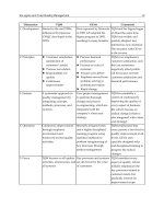
information considered most important are consolidated into a spreadsheet. Table 11
presents the consolidated information including the MiniDMAIC executed on the project
illustrated in this work.
MiniDMAIC: An Approach to Cause and Analysis Resolution in Software Project Development 177

understanding the implemented requirements in accordance with Action 3 were

planned to be held initially. During the sprint 3, the same action was performed again;
 Action 6: this action was planned in the execution of Action 5 and the architectural
component refactoring was performed by the project team, improving the application‘s
maintainability.
The team had difficulty in deploying the action 3 due to the unavailability of an
environment identical to the production environment for the whole team. The other actions
were implemented more easily by the project team. On average, the implementation of the
actions lasted two weeks.

7.6 Performing Phase "Control" of MiniDMAIC
After the implementation of the actions for addressing the causes of defects, the results were
measured to analyze the achieved degree of effectiveness. In the project’s second sprint the
result was measured and we identified 38% of improvement in the systemic tests defect
density indicator and that the result satisfied the project’s limits. Nevertheless, the
established of 81% was not achieved. So we decided to execute the phase “Improvement”,
implementing the same actions in the sprint 3, and measuring the results again to verify if
the actions actually eliminated the root causes of defects.
In the sprint 3 was measured again the defect density in systemic tests indicator and was
found a greater improvement, coming very close to the target defined to the project. Despite
the goal was not achieved in sprint 3, the expected results were considered satisfactory and
we could observe in two later sprints of the projects that the causes of defects were actually
addressed. The improvement in the third sprint was 51%. The Figure 5 shows a control chart
illustrating the improvement achieved by the project over the sprints.

Fig. 5. Project’s Control Chart for Defect Density in Systemic Tests Baseline with Final
Results after the Execution of the MiniDMAIC Action

After the evidence of the implemented improvements, a meeting was held with the team to
collect lessons learned and to close the action with the collected results. As the main lesson
learned from the execution of cause analysis on the project, it was observed the importance,

in the first sprint, to establish a minimum scope that would allow the architecture
development and the knowledge of the team about application’s business domain that was
being developed.

After closing the action, the project coordinator sent the entire MiniDMAIC action
execution‘s input for the organization’s historical basis, through an action in Jira.
Due to the project has being returned to the phase "Improve" to perform the actions in
project’s sprint 3, the MiniDMAIC on the project had a longer duration, approximately 6
weeks. The strategy of re-performing the phase "Improve" on the next sprint of the project
was chosen by the team to check if the actions were really effective and to eliminate the
problem’s root causes. If the project had obtained, actually, an improvement at the first
moment, the duration of the MiniDMAIC action would be, on average, from two to three
weeks.

7.7 Providing Improvement Opportunities for the Organizational Assets
All organization’s MiniDMAIC actions are reviewed and consolidated by the process group
and measurement and analysis group of the organization. The Jira tool generates a
document, in Word format, for every execution of MiniDMAIC action that is sent to the
historical basis by the project and published in a knowledge management tool, becoming
able to be searched by all organization’s projects.
To facilitate the monitoring of all MiniDMAIC actions by the process group, some
information considered most important are consolidated into a spreadsheet. Table 11
presents the consolidated information including the MiniDMAIC executed on the project
illustrated in this work.
Quality Management and Six Sigma178
Type of
Problem
Problem’s Causes Actions Executed for
Addressing the Cause
Achieved

Improvement
High Defect
Density in
Systemic Tests
- Cause 1: architectural
components developed in
parallel with use cases.
- Cause 2: baseline
generated without testing
in an environment similar
to production
environment.
- Cause 3: lack of
understanding of
requirements by
developers.
- Cause 4: Sprint’s scope
badly estimated
(estimation and sequence
of use cases
development).
- Cause 5: architecture is
not suitable for the
concurrent development
of the team.

- Action 1: perform
integration tests before
systemic tests.
- Action 2: held a requirement

workshop for improving the
understanding of the use
cases by the project team.
- Action 3: carry out use case
tests in an environment
similar to the production
environment.
- Action 4: define and
communicate the concept of
"done" to complete the
implementation of the use
case.
- Action 5: improve the
planning to the next
iterations, with the
participation of the team (the
planning should include the
development and integration
of architectural components
before the development of the
use cases).
- Action 6: perform the
refactoring of architectural
components.
Defect density
reduction in 51%

Table 11. Consolidated Information from MiniDMAICs

7.8 Benefits of the MiniDMAIC Approach

Some of the main benefits identified during the execution of MiniDMAIC actions in
software development projects were:
 The execution of MiniDMAIC in the organization, reduced considerably, on the
projects context, the defect density in systemic tests, as reported in Bezerra (2009b) and
increased the productivity as described in Bezerra (2009a);
 The classification of defects used on the approach and adapted by the organization was
essential for helping the projects to understanding the defects and to identify of root
causes;
 The analysis of many MiniDMAIC is fundamental to identify improvement
opportunities for the processes at the organizational level. Thus, we observed that,
according to the organization’s maturity level, new data sources can aggregate greatly

to the processes improvements. These new sources can be added to the list of data that
can be analyzed, defined in Albuquerque (2008);
 The approach implemented in the Jira tool facilitated the use and increased the speed
of MiniDMAIC execution, because this tool already contains all the required fields to
perform each phase;
 Intensifying the use of the action in the projects an improvement was implemented, the
execution of MiniDMAIC in the first set of tests of the projects to analyze the causes of
defects. If the project has none actions to be executed to address the defects, the
MiniDMAIC could be completed in phase "Analyze";
 The template for analyzing the causes of defects in systemic tests, available from the
approach, was of great importance in facilitating the process of analysis and
prioritization of the problem’s root causes addressed in the projects;
 Integration of MiniDMAIC approach to the processes that deal with identifying and
implementing process improvements at the organizational level.

8. Related Works
According to Kalinowski (2009), the first approach to analysis of causes found was
described by Endres (1975), in IBM. This approach deals with individual analysis of

software defects so that they can be categorized and their causes identified, allowing taking
actions to prevent its occurrence in future projects, or at least ensuring its detection in these
projects. The analysis of defects in this approach occurs occasionally, as well as corrective
actions.
The technique RCA (Root Cause Analysis) (Ammerman, 1998), which is one of the
techniques used to analyze the root cause of a problem, aims at formulating
recommendations to eliminate or reduce the incidence of the most recurrent errors and hose
with higher cost in organization’s software development projects. According to Robitaille
(2004), the RCA has the purpose of investigating the factors that are not so visible that has
contributed to the identification of nonconformities or potential problems.
Triz (Altshuller, 1999) is another methodology developed for analysing causes. It is a
systematic human-oriented approach and based on knowledge. His theory defines the
problems where the solution raises new problems.
Card (2005) presents an approach for causal analysis of defects that is summarized in six
steps: (i) select a sample of the defects, (ii) classify the selected defects, (iii) identify
systematic errors, (iv) identify the main causes (V) develop action items, and (vi) record the
results of the causal analysis meeting.
Kalinovski (2009) also describes an approach called DBPI (Defect Based Process
Improvement), and is based on a rich systematic review for elaboration of the approach to
organizational analysis of causes.
Gonçalves (2008b) proposes a causal analysis approach, developed based on the PDCA
method, that applies the multicriteria decision support methodology, aiming to assist the
analysis of causes form complex problems in the context of software organizations.
ISO / IEC 12207 (2008) describes a framework for problem-solving process to analyze and
solve problems (including nonconformances) of any nature or source, that are discovered
during the execution of the development, operation, maintenance or other processes.
MiniDMAIC: An Approach to Cause and Analysis Resolution in Software Project Development 179
Type of
Problem
Problem’s Causes Actions Executed for

Addressing the Cause
Achieved
Improvement
High Defect
Density in
Systemic Tests
- Cause 1: architectural
components developed in
parallel with use cases.
- Cause 2: baseline
generated without testing
in an environment similar
to production
environment.
- Cause 3: lack of
understanding of
requirements by
developers.
- Cause 4: Sprint’s scope
badly estimated
(estimation and sequence
of use cases
development).
- Cause 5: architecture is
not suitable for the
concurrent development
of the team.

- Action 1: perform
integration tests before

systemic tests.
- Action 2: held a requirement
workshop for improving the
understanding of the use
cases by the project team.
- Action 3: carry out use case
tests in an environment
similar to the production
environment.
- Action 4: define and
communicate the concept of
"done" to complete the
implementation of the use
case.
- Action 5: improve the
planning to the next
iterations, with the
participation of the team (the
planning should include the
development and integration
of architectural components
before the development of the
use cases).
- Action 6: perform the
refactoring of architectural
components.
Defect density
reduction in 51%

Table 11. Consolidated Information from MiniDMAICs

7.8 Benefits of the MiniDMAIC Approach
Some of the main benefits identified during the execution of MiniDMAIC actions in
software development projects were:
 The execution of MiniDMAIC in the organization, reduced considerably, on the
projects context, the defect density in systemic tests, as reported in Bezerra (2009b) and
increased the productivity as described in Bezerra (2009a);
 The classification of defects used on the approach and adapted by the organization was
essential for helping the projects to understanding the defects and to identify of root
causes;
 The analysis of many MiniDMAIC is fundamental to identify improvement
opportunities for the processes at the organizational level. Thus, we observed that,
according to the organization’s maturity level, new data sources can aggregate greatly

to the processes improvements. These new sources can be added to the list of data that
can be analyzed, defined in Albuquerque (2008);
 The approach implemented in the Jira tool facilitated the use and increased the speed
of MiniDMAIC execution, because this tool already contains all the required fields to
perform each phase;
 Intensifying the use of the action in the projects an improvement was implemented, the
execution of MiniDMAIC in the first set of tests of the projects to analyze the causes of
defects. If the project has none actions to be executed to address the defects, the
MiniDMAIC could be completed in phase "Analyze";
 The template for analyzing the causes of defects in systemic tests, available from the
approach, was of great importance in facilitating the process of analysis and
prioritization of the problem’s root causes addressed in the projects;
 Integration of MiniDMAIC approach to the processes that deal with identifying and
implementing process improvements at the organizational level.

8. Related Works

According to Kalinowski (2009), the first approach to analysis of causes found was
described by Endres (1975), in IBM. This approach deals with individual analysis of
software defects so that they can be categorized and their causes identified, allowing taking
actions to prevent its occurrence in future projects, or at least ensuring its detection in these
projects. The analysis of defects in this approach occurs occasionally, as well as corrective
actions.
The technique RCA (Root Cause Analysis) (Ammerman, 1998), which is one of the
techniques used to analyze the root cause of a problem, aims at formulating
recommendations to eliminate or reduce the incidence of the most recurrent errors and hose
with higher cost in organization’s software development projects. According to Robitaille
(2004), the RCA has the purpose of investigating the factors that are not so visible that has
contributed to the identification of nonconformities or potential problems.
Triz (Altshuller, 1999) is another methodology developed for analysing causes. It is a
systematic human-oriented approach and based on knowledge. His theory defines the
problems where the solution raises new problems.
Card (2005) presents an approach for causal analysis of defects that is summarized in six
steps: (i) select a sample of the defects, (ii) classify the selected defects, (iii) identify
systematic errors, (iv) identify the main causes (V) develop action items, and (vi) record the
results of the causal analysis meeting.
Kalinovski (2009) also describes an approach called DBPI (Defect Based Process
Improvement), and is based on a rich systematic review for elaboration of the approach to
organizational analysis of causes.
Gonçalves (2008b) proposes a causal analysis approach, developed based on the PDCA
method, that applies the multicriteria decision support methodology, aiming to assist the
analysis of causes form complex problems in the context of software organizations.
ISO / IEC 12207 (2008) describes a framework for problem-solving process to analyze and
solve problems (including nonconformances) of any nature or source, that are discovered
during the execution of the development, operation, maintenance or other processes.
Quality Management and Six Sigma180

Most of the research cited in this work proposes approaches for analysis of causes focusing
on the organizational level. However, it is often necessary to perform analysis of causes
within the projects that must be quick and effective. In organizations seeking high levels of
maturity models of process improvement like CMMI, this practice has to be executed within
the project to maintain the adherence to the model. Furthermore, from the investigated
approaches involving analysis and resolution of causes, none is based on DMAIC method.
The approach presented in this work has the main difference from other approaches the
focus of causal analysis in the context of projects, providing a structured set of steps based
on the DMAIC method, that are simple to execute.

9. Conclusion
The treatment of problems and defects found in software projects is still deficient in most
organizations. The analysis, commonly, do not focus sufficiently on the problem and its
possible sources, leading to wrong decisions, which will ultimately not solve the problem. It
is also difficult to implement a causal analysis and resolution process (CAR) in projects, as
prescribed by the CMMI level 5, due to limited resources which they have to work.
The approach presented in the work aims to minimize these difficulties by proposing a
consistent approach to analysis and resolution of causes based on the DMAIC method, that
is already consolidated in the market. This proposed approach is also adherent to the
process area Causal Analysis and Resolution – CAR of CMMI. Moreover, the approach was
implemented in a workflow tool, and has been executed in several software development
projects in an organization assessed in level 5 of CMMI.
As the main limitation of the approach we have that the MiniDMAIC was defined in the
context of organizations that are at least level 4 of CMMI maturity model, since the
MiniDMAIC actions will have even better results, because several parameters to measure
the projects’ results will be already defined, and the use of statistical analysis tools will
already be a common practice in the organization. However, it can be executed in less
mature organizations, adapting the approach to the organization’s reality, but some steps
may not get the expected results.

10. References
Albuquerque, A. B. (2008). Evaluation and improvement of Organizational Processes Assets
in Software Development Environment. D.Sc. Thesis, COPPE/UFRJ, Rio de Janeiro,
RJ, Brazil.
Altshuller, G. (1999). Innovation Algorithm: TRIZ, systematic innovation and technical
creativity. Technical Innovation Ctr.
Ammerman, M. (1998). The Root Cause Analysis Handbook: A Simplified Approach to
Identifying, Correcting, and Reporting Workplace Errors. Productivity Press.
Banas Qualidade. (2007). “Continuous improvement – Soluctions to Problems”, Quality
News. São Paulo. Accessible in
/>. Acessed in: 2007, Feb 22.

Bezerra, C. I. M.; Coelho, C.; Gonçalves, F. M.; Giovano, C.; Albuquerque, A. B. (2009a).
MiniDMAIC: An Approach to Causal Analysis and Resolution in Software
Development Projects. VIII Brazilian Simposium on Software Quality, Ouro Preto.
Proceedings of the VIII Brazilian Simposium on Software Quality.
Bezerra, C. I. M. (2009b). MiniDMAIC: An Approach to Causal Analysis and Resolution in
Software Development Projects. Master Dissertation, University of Fortaleza
(UNIFOR), Fortaleza, Ceará, Brazil.
Blauth, Regis. (2003). Six Sigma: a strategy for improving results, FAE Business Journal, nº 5.
Card, D. N. (2005). Defect Analysis: Basic Techniques for Management and Learning,
Advances in Computers 65.
Chillarege, R. et al. (1992). Orthogonal Defect Classification: a Concept for in-Process
Measurements. IEEE Transactions on SE, v.18, n. 11, pp 943-956.
Chrissis, Mary B.; Konrad, Mike; Shrum, Sandy. (2006). CMMI: Guidelines for Process
Integration and Product Improvement, 2nd edition, Boston, Addison Wesley.
Dennis, M. (1994). The Chaos Study, The Standish Group International.
Endres, A. (1975). An Analysis of Errors and Their Causes in Systems Programs, IEEE
Transactions on Software Engineering, SE-1, 2, June 1975, pp. 140-149.
Gonçalves, F., Bezerra, C., Belchior, A., Coelho, C., Pires, C. (2008a). Implementing Causal

Analysis and Resolution in Software Development Projects: The MiniDMAIC
Approach, 19th Australian Conference on Software Engineering, pp. 112-119.
Gonçalves, F. (2008b) An Approach to Causal Analysis and Resolution of Problems Using
Multicriteria. Master Dissertation, University of Fortaleza (UNIFOR), Fortaleza,
Ceará, Brazil.
IEEE standard classification for software anomalies (1944). IEEE Std 1044-1993. 2 Jun 1994.
ISO/IEC 12207:1995/Amd 2:2008, (2008). Information Technology - Software Life Cycle
Process, Amendment 2. Genebra: ISO.
Ishikawa, K. (1985). What is Total Quality Control? The Japanese Way. Prentice Hall.
Juran, J. M. (1991). Qualtiy Control, Handbook. J. M. Juran, Frank M. Gryna - São Paulo -
Makron, McGraw-Hill.
Kalinowski, M. (2009) “DBPI: Approach to Prevent Defects in Software to Support the
Improvement in Processes and Organizational Learning”. Qualifying Exam,
COPPE/UFRJ, Rio de Janeiro, RJ, Brazil.
Kulpa, Margaret K.; Johnson, Kent A. (2003). Interpreting the CMMI: a process improvent
approach. Florida, Auerbach.
Pande, S. (2001). Six Sigma Strategy: how the GE, the Motorola and others big comnpanies
are sharpening their performance. Rio de Janeiro, Qualitymark.
Rath and Strong. (2005). Six Sigma/DMAIC Road Map, 2nd edition.
Robitaille, D. (2004). Root Cause Analysis: Basic Tools and Techniques. Chico, CA: Paton
Press.
Rotondaro, G. R; Ramos, A. W.; Ribeiro, C. O.; Miyake, D. I.; Nakano, D.; Laurindo, F. J. B;
Ho, L. L.; Carvalho, M. M.; Braz, A. A.; Balestrassi, P. P. (2002). Six Sigma:
Management Strategy for Improving Processes, Products and Services, São Paulo,
Atlas.
Smith, B.; Adams, E. (2000). LeanSigma: advanced quality, Proc. 54th Annual Quality
Congress of the American Society for Quality, Indianapolis, Indiana.
MiniDMAIC: An Approach to Cause and Analysis Resolution in Software Project Development 181

Most of the research cited in this work proposes approaches for analysis of causes focusing

on the organizational level. However, it is often necessary to perform analysis of causes
within the projects that must be quick and effective. In organizations seeking high levels of
maturity models of process improvement like CMMI, this practice has to be executed within
the project to maintain the adherence to the model. Furthermore, from the investigated
approaches involving analysis and resolution of causes, none is based on DMAIC method.
The approach presented in this work has the main difference from other approaches the
focus of causal analysis in the context of projects, providing a structured set of steps based
on the DMAIC method, that are simple to execute.

9. Conclusion
The treatment of problems and defects found in software projects is still deficient in most
organizations. The analysis, commonly, do not focus sufficiently on the problem and its
possible sources, leading to wrong decisions, which will ultimately not solve the problem. It
is also difficult to implement a causal analysis and resolution process (CAR) in projects, as
prescribed by the CMMI level 5, due to limited resources which they have to work.
The approach presented in the work aims to minimize these difficulties by proposing a
consistent approach to analysis and resolution of causes based on the DMAIC method, that
is already consolidated in the market. This proposed approach is also adherent to the
process area Causal Analysis and Resolution – CAR of CMMI. Moreover, the approach was
implemented in a workflow tool, and has been executed in several software development
projects in an organization assessed in level 5 of CMMI.
As the main limitation of the approach we have that the MiniDMAIC was defined in the
context of organizations that are at least level 4 of CMMI maturity model, since the
MiniDMAIC actions will have even better results, because several parameters to measure
the projects’ results will be already defined, and the use of statistical analysis tools will
already be a common practice in the organization. However, it can be executed in less
mature organizations, adapting the approach to the organization’s reality, but some steps
may not get the expected results.

10. References

Albuquerque, A. B. (2008). Evaluation and improvement of Organizational Processes Assets
in Software Development Environment. D.Sc. Thesis, COPPE/UFRJ, Rio de Janeiro,
RJ, Brazil.
Altshuller, G. (1999). Innovation Algorithm: TRIZ, systematic innovation and technical
creativity. Technical Innovation Ctr.
Ammerman, M. (1998). The Root Cause Analysis Handbook: A Simplified Approach to
Identifying, Correcting, and Reporting Workplace Errors. Productivity Press.
Banas Qualidade. (2007). “Continuous improvement – Soluctions to Problems”, Quality
News. São Paulo. Accessible in
Acessed in: 2007, Feb 22.

Bezerra, C. I. M.; Coelho, C.; Gonçalves, F. M.; Giovano, C.; Albuquerque, A. B. (2009a).
MiniDMAIC: An Approach to Causal Analysis and Resolution in Software
Development Projects. VIII Brazilian Simposium on Software Quality, Ouro Preto.
Proceedings of the VIII Brazilian Simposium on Software Quality.
Bezerra, C. I. M. (2009b). MiniDMAIC: An Approach to Causal Analysis and Resolution in
Software Development Projects. Master Dissertation, University of Fortaleza
(UNIFOR), Fortaleza, Ceará, Brazil.
Blauth, Regis. (2003). Six Sigma: a strategy for improving results, FAE Business Journal, nº 5.
Card, D. N. (2005). Defect Analysis: Basic Techniques for Management and Learning,
Advances in Computers 65.
Chillarege, R. et al. (1992). Orthogonal Defect Classification: a Concept for in-Process
Measurements. IEEE Transactions on SE, v.18, n. 11, pp 943-956.
Chrissis, Mary B.; Konrad, Mike; Shrum, Sandy. (2006). CMMI: Guidelines for Process
Integration and Product Improvement, 2nd edition, Boston, Addison Wesley.
Dennis, M. (1994). The Chaos Study, The Standish Group International.
Endres, A. (1975). An Analysis of Errors and Their Causes in Systems Programs, IEEE
Transactions on Software Engineering, SE-1, 2, June 1975, pp. 140-149.
Gonçalves, F., Bezerra, C., Belchior, A., Coelho, C., Pires, C. (2008a). Implementing Causal
Analysis and Resolution in Software Development Projects: The MiniDMAIC

Approach, 19th Australian Conference on Software Engineering, pp. 112-119.
Gonçalves, F. (2008b) An Approach to Causal Analysis and Resolution of Problems Using
Multicriteria. Master Dissertation, University of Fortaleza (UNIFOR), Fortaleza,
Ceará, Brazil.
IEEE standard classification for software anomalies (1944). IEEE Std 1044-1993. 2 Jun 1994.
ISO/IEC 12207:1995/Amd 2:2008, (2008). Information Technology - Software Life Cycle
Process, Amendment 2. Genebra: ISO.
Ishikawa, K. (1985). What is Total Quality Control? The Japanese Way. Prentice Hall.
Juran, J. M. (1991). Qualtiy Control, Handbook. J. M. Juran, Frank M. Gryna - São Paulo -
Makron, McGraw-Hill.
Kalinowski, M. (2009) “DBPI: Approach to Prevent Defects in Software to Support the
Improvement in Processes and Organizational Learning”. Qualifying Exam,
COPPE/UFRJ, Rio de Janeiro, RJ, Brazil.
Kulpa, Margaret K.; Johnson, Kent A. (2003). Interpreting the CMMI: a process improvent
approach. Florida, Auerbach.
Pande, S. (2001). Six Sigma Strategy: how the GE, the Motorola and others big comnpanies
are sharpening their performance. Rio de Janeiro, Qualitymark.
Rath and Strong. (2005). Six Sigma/DMAIC Road Map, 2nd edition.
Robitaille, D. (2004). Root Cause Analysis: Basic Tools and Techniques. Chico, CA: Paton
Press.
Rotondaro, G. R; Ramos, A. W.; Ribeiro, C. O.; Miyake, D. I.; Nakano, D.; Laurindo, F. J. B;
Ho, L. L.; Carvalho, M. M.; Braz, A. A.; Balestrassi, P. P. (2002). Six Sigma:
Management Strategy for Improving Processes, Products and Services, São Paulo,
Atlas.
Smith, B.; Adams, E. (2000). LeanSigma: advanced quality, Proc. 54th Annual Quality
Congress of the American Society for Quality, Indianapolis, Indiana.
Quality Management and Six Sigma182

Siviy, J. M.; Penn, L. M.; Happer, E. (2005). Relationship Between CMMI and Six Sigma.
Techical Note, CMU / SEI -2005-TN-005.

Tayntor, Christine B. (2003). Six Sigma Software Development, Flórida, Auerbach.
Watson, G. H. (2001). Cycles of learning: observations of Jack Welch, ASQ Publication.
Dening Placement Machine Capability by Using Statistical Methods 183
Dening Placement Machine Capability By Using Statistical Methods
Timo Liukkonen, Ph.D
X

Defining Placement Machine Capability
by Using Statistical Methods

Timo Liukkonen, Ph.D. (Eng.)
Nokia Corporation
Finland

1. Introduction
Modern placement machine’s capability to place certain electrical components can be
defined as a question of required accuracy. In six sigma methodology the discussion about
accuracy is divided into accuracy and precision. Accuracy can be defined as the closeness of
agreement between an observed value and the accepted reference value and it is usually
referred as an offset value, see Fig.1. Precision is often used to describe the expected
variation of repeated measurements over the range of measurement, see Fig.2, and can also
be further broken into two components: repeatability and reproducibility (Breyfogle, 2003).



Fig. 1. Definition of accuracy: Process X
A
has lower accuracy than process X
B
i.e.

process
X
A
has bigger offset from reference line. Both have approximately the same precision.

In common everyday language the word accuracy is often used to mean both accuracy and
precision at the same time: machine is accurate when both its offset from reference and its
variation are small. A rifle e.g. can be said to be “accurate” when all ten bullet holes are
found between scores 9.75 and 10.00, but mathematically the shooting process, including
also the shooter and conditions, is both accurate and precise.
10
Quality Management and Six Sigma184

Fig. 2. Definition of precision: Process X
A
has better precision (less variation) than process
X
B
. Both processes have approximately the same accuracy (same offset from reference line).

2. Placement machine accuracy and former studies
Rotary turret SMD (Surface Mounted Device) placement machine (Fig.3) has moving XY-
table to transfer Printed Wiring Board (PWB) to correct position below the placement head.
XY-table moves also in vertical direction to adjust placement height to various component
thicknesses. Component feeders are arranged behind the machine in a table, which transfers
the correct feeder below the placement head. Placement heads with various sizes of vacuum
nozzles are arranged in the turret, which revolves and moves pickup nozzles from part
pickup point to placement point in a continuos movement providing vision inspection and
rotational correction on the way.

Fig. 3. Principle of a rotary turret placement machine (Johnsson, 1999).

Placement defects such as misaligned or missing parts on PWB are expensive when
reworked after reflow soldering. Naturally good quality of the preceding solder paste
printing process is crucial for successful component placement (Liukkonen & Tuominen,
2004). One cause for placement defect is poor placement accuracy of the placement machine
(Kalen, 2002; Kamen, 1998). Controlling of placement accuracy has a significant role in
placement quality and becomes even more important when placement machines gain more
operation hours (Liukkonen & Tuominen, 2003).

CeTaq GmbH provides placement capability analysis services for electronics manufacturing
field. In order to reduce the extra variation coming from e.g. inaccurate materials CeTaq
GmbH uses special glass components and glass boards, as well as dedicated camera based
measuring device for the results (Sivigny, 2007; Sauer et al., 1998). In this six sigma study the
purpose is to use commercial standard components and very simple FR4 type glas epoxy
PWB. Problem with special materials is the extra cost and extra time needed to prepare and
perform the test under the special circumstances. By using standard materials we can keep
the cost down and also speed up the time needed for the testing when e.g. the same board
thickness and size can be used as normally in the production line. This will make it easier
for the line engineers to start the test when needed because it takes only 15-30 minutes.
Kamen has studied the factors affecting SMD placement accuracy, but has put especially
focus on effects coming from variations in solder paste printing, vertical placement force
and different component types, whereas in this study they all are considered and kept more
or less as constant (Kamen, 1998). Wischoffer discusses about correct component alignment
and possible offsets after placement and points out four factors that affect the most: part
mass, part height, lead area contacting solder paste and solder paste viscosity (Wischoffer,
2003). Baker studies also the factors affecting placement accuracy and highlights that limits
used in placement machine parameters should be defined separately by each company and

are based on economics on machine cost, process cost, overall production cost, repair cost
and the cost having a defective or potentially defective product reach the customer (Baker,
1996). In this study the technical limits are set by the technical acceptance for the new
technology requirements coming from the company.

CeTaq GmbH defines the purpose of capability measurements in three different customer
groups as shown in Table 1 (CeTaq, 2010). For this project the main purpose well aligned
with CeTaq’s grouping can be found in Technical acceptance and machine qualification.

Equipment Retailer Distribute
r
Customer-
Manufacturer -After Sales Service Desi
g
ner - Auditors
-Electronic Manufacturer
-OEM
-Design -Technical Acceptance -Audits
-Validation and machine -Quality management
-DOE Qualification systems
-Machine qualification -Line Configuration -Design for
before shipping -Maintenance optimization manufacturability
… -Statistical Process …
Control
-Task force / Six sigma
-Customer report on
demand
-Identify root-causes
for Quality issues
…

Table 1. Capability measurements defined in three customer groups (CeTaq, 2010).

Dening Placement Machine Capability by Using Statistical Methods 185

Fig. 2. Definition of precision: Process X
A
has better precision (less variation) than process
X
B
. Both processes have approximately the same accuracy (same offset from reference line).

2. Placement machine accuracy and former studies
Rotary turret SMD (Surface Mounted Device) placement machine (Fig.3) has moving XY-
table to transfer Printed Wiring Board (PWB) to correct position below the placement head.
XY-table moves also in vertical direction to adjust placement height to various component
thicknesses. Component feeders are arranged behind the machine in a table, which transfers
the correct feeder below the placement head. Placement heads with various sizes of vacuum
nozzles are arranged in the turret, which revolves and moves pickup nozzles from part
pickup point to placement point in a continuos movement providing vision inspection and
rotational correction on the way.


Fig. 3. Principle of a rotary turret placement machine (Johnsson, 1999).

Placement defects such as misaligned or missing parts on PWB are expensive when
reworked after reflow soldering. Naturally good quality of the preceding solder paste
printing process is crucial for successful component placement (Liukkonen & Tuominen,
2004). One cause for placement defect is poor placement accuracy of the placement machine
(Kalen, 2002; Kamen, 1998). Controlling of placement accuracy has a significant role in

placement quality and becomes even more important when placement machines gain more
operation hours (Liukkonen & Tuominen, 2003).

CeTaq GmbH provides placement capability analysis services for electronics manufacturing
field. In order to reduce the extra variation coming from e.g. inaccurate materials CeTaq
GmbH uses special glass components and glass boards, as well as dedicated camera based
measuring device for the results (Sivigny, 2007; Sauer et al., 1998). In this six sigma study the
purpose is to use commercial standard components and very simple FR4 type glas epoxy
PWB. Problem with special materials is the extra cost and extra time needed to prepare and
perform the test under the special circumstances. By using standard materials we can keep
the cost down and also speed up the time needed for the testing when e.g. the same board
thickness and size can be used as normally in the production line. This will make it easier
for the line engineers to start the test when needed because it takes only 15-30 minutes.
Kamen has studied the factors affecting SMD placement accuracy, but has put especially
focus on effects coming from variations in solder paste printing, vertical placement force
and different component types, whereas in this study they all are considered and kept more
or less as constant (Kamen, 1998). Wischoffer discusses about correct component alignment
and possible offsets after placement and points out four factors that affect the most: part
mass, part height, lead area contacting solder paste and solder paste viscosity (Wischoffer,
2003). Baker studies also the factors affecting placement accuracy and highlights that limits
used in placement machine parameters should be defined separately by each company and
are based on economics on machine cost, process cost, overall production cost, repair cost
and the cost having a defective or potentially defective product reach the customer (Baker,
1996). In this study the technical limits are set by the technical acceptance for the new
technology requirements coming from the company.

CeTaq GmbH defines the purpose of capability measurements in three different customer
groups as shown in Table 1 (CeTaq, 2010). For this project the main purpose well aligned
with CeTaq’s grouping can be found in Technical acceptance and machine qualification.

Equipment Retailer Distribute
r
Customer-
Manufacturer -After Sales Service Desi
g
ner - Auditors
-Electronic Manufacturer
-OEM
-Design -Technical Acceptance -Audits
-Validation and machine -Quality management
-DOE Qualification systems
-Machine qualification -Line Configuration -Design for
before shipping -Maintenance optimization manufacturability
… -Statistical Process …
Control
-Task force / Six sigma
-Customer report on
demand
-Identify root-causes
for Quality issues
…

Table 1. Capability measurements defined in three customer groups (CeTaq, 2010).

Quality Management and Six Sigma186
3. The DEFINE phase in a Six Sigma project
This study was completed like a six sigma project including the identifiable DMAIC-process
phases: D
efine, Measure, Analyse, Improve and Control (Breyfogle, 2003). However,
because this project is quite short some phases like analyze and improve were combined

partly together already in the beginning of planning the experiments. Design Of
Experiments (DOE), a statistical tool used to screen the factors to determine which are
important for explaining process variation (Montgomery, 2008), has been mostly presented
in the Analysis chapters and the interactions found there are presented in Improve phase.

3.1 Selection of the project and the voice of the customer
Project selection is the most important part of a Define phase in a six sigma project. In this
project the purpose was to find out what is minimum placement machine’s Sigma Quality
Level (later also referred as Placement Sigma Level, PSL) that still produces good placement
quality when spacing between the components on the PWB will be decreased by 33%.
Customer’s plan to decrease component spacing by 33% may be too demanding for, at least,
those machines which have a lower placement sigma level in placement accuracy, but are
still assumed to be used in production for several years. This leads to the second important
part of the Define phase, to the business case behind the selected project (Breyfogle, 2003): a
lot of bad Quality may be produced if the most capable machines can not be selected. At the
same time new investments in machinery can be postponed in the future which will bring
additional economical value. Therefore ranking of the available machines is essential.

The smallest component to be assembled is 0402 size capacitor and resistor, where the
nominal length of the component is 1mm and width 0.5mm. The height of a resistor is
0.3mm and that of the capacitor is 0.5mm. Because the required placement nozzle is wider
than the 0402 component, , it may be necessary to place all resistors first before any of the
taller capacitors to prevent the protruding nozzle hitting the components already been
placed, i.e. place components according to their height. When component-to-component
spacing is larger the problem arising from protruding nozzle does not matter. The kind of
“forced” placement sequence will deteriorate free placement optimization and will then
have negative effect on line output and also on placement quality as has been shown in
previous publications (Liukkonen & Tuominen, 2003).

3.2 Problem Statement

It is essential to determine the project scope in relation to business case and also to available
project resources. Primary target of this study is to rank the placement machines according
to their capability to place high-density 0402s i.e. what is the minimum requirement in terms
of sigma quality level? Secondary target is to verify the need for forced placement sequence:
should all resistors be placed before any taller capacitors?

4. Process Exploration: the MEASURE phase
4.1 Response Variables and Metrics
In six sigma projects the monitored process outputs are divided into variable type data and
attribute type data. Variable data is quantitative data (continuous data) where
measurements are used for analysis, e.g. shaft diameter in millimeters. Attribute data is
qualitative data that can be counted for recording and analysis. Examples include
characteristics such as “missing” or “present”, “good” or “bad”, “accepted” or “rejected”.
Attribute data can also include characteristics that are inherently measurable but where
results are finally recorded in a simple yes/no or go/no-go fashion (AIAG, 1995). According
to six sigma the process output (response) is a function of process inputs (e.g. materials or
process setup parameters) i.e. Y=f(X). In this study the following responses are monitored.

Attribute data type responses:
Placement errors
Referred later in Figures as Y1 e.g. missing, misaligned, skewed
- Specification used for category “Misaligned” in placement errors before
reflow soldering: +/- 180 µm for 0402 components

Variable data type responses:
Placement position against nominal in X and Y axes i.e. ΔX, ΔY
X Mean (referred later in Figures as Y
21
)
X StDev (standard deviation, referred later in Figures as Y

22
)
Y Mean (referred later in Figures as Y
23
)

Y StDev (standard deviation, referred later in Figures as Y
24
)


Specification for Means: +/- 100 µm (at 3 sigmas, machine manufacturer’s specification)
Specification for StDevs: +/- 33 µm (tolerance area /6, i.e. 200 µm / 6)

4.2 Measurement System Analysis
Measurement system description The optical-based AOI (automated optical inspection)
system used in this study utilizes solid shape modeling to measure and characterize
components and solder joints with lifelike 3D visualization. System has 20-25 µm/pixel
resolution at all times with a single high-resolution digital camera and high-speed precision
XY-robot. The very same AOI machine was used throughout the study and the machine was
calibrated by the manufacturer before the study. Post-placement inspection tools are
common sight in a modern SMT (Surface Mount Technology) production line today, and
these in-line tools are very often also utilized in various placement accuracy tests and
evaluations (Kamen, 1998).

Measurement system Gage
For repeatability test (precision) of the AOI five populated PWB panels were measured with
pre-reflow AOI, each three times, totally including 13 680 observations. Gage test was based
on two randomly selected components. Calculated Gage error result 1.09% was excellent
(see Fig.4) and AOI seemed to be fully capable as a measurement system for the analysis in

this study.
Dening Placement Machine Capability by Using Statistical Methods 187
3. The DEFINE phase in a Six Sigma project
This study was completed like a six sigma project including the identifiable DMAIC-process
phases: Define, Measure, Analyse, Improve and Control (Breyfogle, 2003). However,
because this project is quite short some phases like analyze and improve were combined
partly together already in the beginning of planning the experiments. Design Of
Experiments (DOE), a statistical tool used to screen the factors to determine which are
important for explaining process variation (Montgomery, 2008), has been mostly presented
in the Analysis chapters and the interactions found there are presented in Improve phase.

3.1 Selection of the project and the voice of the customer
Project selection is the most important part of a Define phase in a six sigma project. In this
project the purpose was to find out what is minimum placement machine’s Sigma Quality
Level (later also referred as Placement Sigma Level, PSL) that still produces good placement
quality when spacing between the components on the PWB will be decreased by 33%.
Customer’s plan to decrease component spacing by 33% may be too demanding for, at least,
those machines which have a lower placement sigma level in placement accuracy, but are
still assumed to be used in production for several years. This leads to the second important
part of the Define phase, to the business case behind the selected project (Breyfogle, 2003): a
lot of bad Quality may be produced if the most capable machines can not be selected. At the
same time new investments in machinery can be postponed in the future which will bring
additional economical value. Therefore ranking of the available machines is essential.

The smallest component to be assembled is 0402 size capacitor and resistor, where the
nominal length of the component is 1mm and width 0.5mm. The height of a resistor is
0.3mm and that of the capacitor is 0.5mm. Because the required placement nozzle is wider
than the 0402 component, , it may be necessary to place all resistors first before any of the
taller capacitors to prevent the protruding nozzle hitting the components already been
placed, i.e. place components according to their height. When component-to-component

spacing is larger the problem arising from protruding nozzle does not matter. The kind of
“forced” placement sequence will deteriorate free placement optimization and will then
have negative effect on line output and also on placement quality as has been shown in
previous publications (Liukkonen & Tuominen, 2003).

3.2 Problem Statement
It is essential to determine the project scope in relation to business case and also to available
project resources. Primary target of this study is to rank the placement machines according
to their capability to place high-density 0402s i.e. what is the minimum requirement in terms
of sigma quality level? Secondary target is to verify the need for forced placement sequence:
should all resistors be placed before any taller capacitors?

4. Process Exploration: the MEASURE phase
4.1 Response Variables and Metrics
In six sigma projects the monitored process outputs are divided into variable type data and
attribute type data. Variable data is quantitative data (continuous data) where
measurements are used for analysis, e.g. shaft diameter in millimeters. Attribute data is
qualitative data that can be counted for recording and analysis. Examples include
characteristics such as “missing” or “present”, “good” or “bad”, “accepted” or “rejected”.
Attribute data can also include characteristics that are inherently measurable but where
results are finally recorded in a simple yes/no or go/no-go fashion (AIAG, 1995). According
to six sigma the process output (response) is a function of process inputs (e.g. materials or
process setup parameters) i.e. Y=f(X). In this study the following responses are monitored.

Attribute data type responses:
Placement errors
Referred later in Figures as Y1 e.g. missing, misaligned, skewed
- Specification used for category “Misaligned” in placement errors before
reflow soldering: +/- 180 µm for 0402 components

Variable data type responses:
Placement position against nominal in X and Y axes i.e. ΔX, ΔY
X Mean (referred later in Figures as Y
21
)
X StDev (standard deviation, referred later in Figures as Y
22
)
Y Mean (referred later in Figures as Y
23
)

Y StDev (standard deviation, referred later in Figures as Y
24
)


Specification for Means: +/- 100 µm (at 3 sigmas, machine manufacturer’s specification)
Specification for StDevs: +/- 33 µm (tolerance area /6, i.e. 200 µm / 6)

4.2 Measurement System Analysis
Measurement system description
The optical-based AOI (automated optical inspection)
system used in this study utilizes solid shape modeling to measure and characterize
components and solder joints with lifelike 3D visualization. System has 20-25 µm/pixel
resolution at all times with a single high-resolution digital camera and high-speed precision
XY-robot. The very same AOI machine was used throughout the study and the machine was
calibrated by the manufacturer before the study. Post-placement inspection tools are
common sight in a modern SMT (Surface Mount Technology) production line today, and
these in-line tools are very often also utilized in various placement accuracy tests and

evaluations (Kamen, 1998).

Measurement system Gage

For repeatability test (precision) of the AOI five populated PWB panels were measured with
pre-reflow AOI, each three times, totally including 13 680 observations. Gage test was based
on two randomly selected components. Calculated Gage error result 1.09% was excellent
(see Fig.4) and AOI seemed to be fully capable as a measurement system for the analysis in
this study.
Quality Management and Six Sigma188

Fig. 4. On the Left: AOI Gage error result showing that 0.68% of inaccuracy comes from the
AOI itself on X axis and 1.09% on Y axis. On the Right: Test boards’ coordinate system and
AOI screenshot of 0402 components in 0 placement angle.

For additional reliability a second gage test round was made. Measurements were taken
from all the components separately using two randomly selected PWB panels and entered
into a Boxplot chart. Boxplot is a tool that can visually show differences between
characteristics of a data set. Box plots display the lower and upper quartiles (the 25th and
the 75th percentiles), and the median (the 50
th
percentile) appears as a horizontal line within
the box (Breyfogle, 2003). The analysis produced Fig. 5 where AOI deviation defined as X-
Range (i.e. measured max ΔX value – min ΔX value separately calculated for each circuit
reference) in X axis is large when placement angle 0 is used. Fig. 5 shows that X range is 80
µm with capacitors and 30 µm with resistors. See right part of Fig. 4 for clarification of
placement angles and PWB coordinate system. AOI deviation defined as Y-range in Y axis is
large when angle 270 is used. Fig. 5 shows that Y range is 60 µm with capacitors and 30 µm
with resistors. Because this observed repeatability error was randomly distributed all over
the board area and therefore could not be avoided by deleting certain references it was

decided not to use Y axis data with 270 placement angle and X axis data with 0 angle in
further analysis of this study. Fig. 5 also shows that X axis data with 270 angle and Y axis
data with 0 angle is fully reliable and usable for this study. The gage problem originates
from AOI’s inability to detect component location accurately in its lengthwise direction with
selected algorithm, especially with capacitors. AOI manufacturer was informed about the
observed algorithm problem.

XRange
Board
A ngle
C ompT ype
32
27002700
RCRCRCRC
80
60
40
20
0
YRa nge
Board
A ngle
C ompT ype
32
27002700
RCRCRCRC
60
45
30
15

0
Boxplot of XRange vs Board, Angle, CompType
Wo rkshee t: XSt atistics
Boards 2 and 3 X
Boxplot of YRange vs Board, Angle, CompType
Wo rkshee t: YSt a tistics
Boards 2 and 3 Y



  
  

 


XRange
Board
A ngle
C ompT ype
32
27002700
RCRCRCRC
80
60
40
20
0
YRa nge
Board

A ngle
C ompT ype
32
27002700
RCRCRCRC
60
45
30
15
0
Boxplot of XRange vs Board, Angle, CompType
Wo rkshee t: XSt atistics
Boards 2 and 3 X
Boxplot of YRange vs Board, Angle, CompType
Wo rkshee t: YSt a tistics
Boards 2 and 3 Y



  
  

 



Fig. 5. Boxplot of range for ΔX (XRange) and ΔY (YRange) in relation to board, placement
angle and component type, including categorization of repeatability results into “Good =
Happy-Face”, “OK = Neutral-Face” and “Not Used = Sad-Face” symbols showing the
goodness levels. Range values shown in

µm, angles in degrees. C=Capacitor, R=Resistor.

4.3 Process Map
It is advantageous to represent system structure and relationships using flowcharts. This
provides a complete pictorial sequence of what happens from start to finish of a procedure
in order to e.g. identify opportunities for improvement and identify key process input
variables. An alternative to flowchart is higher level process map that shows only a few
major process steps as activity symbols (Breyfogle, 2003). The process map of a turret type
placement machine is shown in Fig.6. The two main areas where input parameters in this
study are affecting the process are “X/Y table moves to placement position” and “head
comes down to placement height”. The process map is created by the six sigma project team.

Device table moves
feeder to pickup
position
Head comes down
and suction is
activated in nozzle
Tape feed lever comes
down and feeding is
performed
component is
picked up
tape cutter
cuts the
carrier tape
Nozzle
comes
up
Pre-rotation is

done (if needed)
Component i s
recognized by
camera
Rotation (Q) i s
corrected
X/Y-table
moves to
placement
position
Head comes
down to
placement height
Suction is turned
off and blow on
Component is
placed on PWB
Component i s
rejected by
camera
Component i s
missing
AOI measurement:
Y1, Y2 (Y
21
, Y
22
, Y
23
,

Y
24
)
Project X’s
affect in
these steps
Device table moves
feeder to pickup
position
Head comes down
and suction is
activated in nozzle
Tape feed lever comes
down and feeding is
performed
component is
picked up
tape cutter
cuts the
carrier tape
Nozzle
comes
up
Pre-rotation is
done (if needed)
Component i s
recognized by
camera
Rotation (Q) i s
corrected

X/Y-table
moves to
placement
position
Head comes
down to
placement height
Suction is turned
off and blow on
Component is
placed on PWB
Component i s
rejected by
camera
Component i s
missing
AOI measurement:
Y1, Y2 (Y
21
, Y
22
, Y
23
,
Y
24
)
Device table moves
feeder to pickup
position

Head comes down
and suction is
activated in nozzle
Tape feed lever comes
down and feeding is
performed
component is
picked up
tape cutter
cuts the
carrier tape
Nozzle
comes
up
Pre-rotation is
done (if needed)
Component i s
recognized by
camera
Rotation (Q) i s
corrected
X/Y-table
moves to
placement
position
Head comes
down to
placement height
Suction is turned
off and blow on

Component is
placed on PWB
Component i s
rejected by
camera
Component i s
missing
AOI measurement:
Y1, Y2 (Y
21
, Y
22
, Y
23
,
Y
24
)
Project X’s
affect in
these steps

Fig. 6. Component pickup and placement process mapping.
Dening Placement Machine Capability by Using Statistical Methods 189

Fig. 4. On the Left: AOI Gage error result showing that 0.68% of inaccuracy comes from the
AOI itself on X axis and 1.09% on Y axis. On the Right: Test boards’ coordinate system and
AOI screenshot of 0402 components in 0 placement angle.

For additional reliability a second gage test round was made. Measurements were taken

from all the components separately using two randomly selected PWB panels and entered
into a Boxplot chart. Boxplot is a tool that can visually show differences between
characteristics of a data set. Box plots display the lower and upper quartiles (the 25th and
the 75th percentiles), and the median (the 50
th
percentile) appears as a horizontal line within
the box (Breyfogle, 2003). The analysis produced Fig. 5 where AOI deviation defined as X-
Range (i.e. measured max ΔX value – min ΔX value separately calculated for each circuit
reference) in X axis is large when placement angle 0 is used. Fig. 5 shows that X range is 80
µm with capacitors and 30 µm with resistors. See right part of Fig. 4 for clarification of
placement angles and PWB coordinate system. AOI deviation defined as Y-range in Y axis is
large when angle 270 is used. Fig. 5 shows that Y range is 60 µm with capacitors and 30 µm
with resistors. Because this observed repeatability error was randomly distributed all over
the board area and therefore could not be avoided by deleting certain references it was
decided not to use Y axis data with 270 placement angle and X axis data with 0 angle in
further analysis of this study. Fig. 5 also shows that X axis data with 270 angle and Y axis
data with 0 angle is fully reliable and usable for this study. The gage problem originates
from AOI’s inability to detect component location accurately in its lengthwise direction with
selected algorithm, especially with capacitors. AOI manufacturer was informed about the
observed algorithm problem.

XRange
Board
A ngle
C ompT ype
32
27002700
RCRCRCRC
80
60

40
20
0
YRa nge
Board
A ngle
C ompT ype
32
27002700
RCRCRCRC
60
45
30
15
0
Boxplot of XRange vs Board, Angle, CompType
Wo rkshee t: XSt atistics
Boards 2 and 3 X
Boxplot of YRange vs Board, Angle, CompType
Wo rkshee t: YSt a tistics
Boards 2 and 3 Y



  
  

 



XRange
Board
A ngle
C ompT ype
32
27002700
RCRCRCRC
80
60
40
20
0
YRa nge
Board
A ngle
C ompT ype
32
27002700
RCRCRCRC
60
45
30
15
0
Boxplot of XRange vs Board, Angle, CompType
Wo rkshee t: XSt atistics
Boards 2 and 3 X
Boxplot of YRange vs Board, Angle, CompType
Wo rkshee t: YSt a tistics
Boards 2 and 3 Y




  
  

 



Fig. 5. Boxplot of range for ΔX (XRange) and ΔY (YRange) in relation to board, placement
angle and component type, including categorization of repeatability results into “Good =
Happy-Face”, “OK = Neutral-Face” and “Not Used = Sad-Face” symbols showing the
goodness levels. Range values shown in
µm, angles in degrees. C=Capacitor, R=Resistor.

4.3 Process Map
It is advantageous to represent system structure and relationships using flowcharts. This
provides a complete pictorial sequence of what happens from start to finish of a procedure
in order to e.g. identify opportunities for improvement and identify key process input
variables. An alternative to flowchart is higher level process map that shows only a few
major process steps as activity symbols (Breyfogle, 2003). The process map of a turret type
placement machine is shown in Fig.6. The two main areas where input parameters in this
study are affecting the process are “X/Y table moves to placement position” and “head
comes down to placement height”. The process map is created by the six sigma project team.

Device table moves
feeder to pickup
position
Head comes down

and suction is
activated in nozzle
Tape feed lever comes
down and feeding is
performed
component is
picked up
tape cutter
cuts the
carrier tape
Nozzle
comes
up
Pre-rotation is
done (if needed)
Component i s
recognized by
camera
Rotation (Q) i s
corrected
X/Y-table
moves to
placement
position
Head comes
down to
placement height
Suction is turned
off and blow on
Component is

placed on PWB
Component i s
rejected by
camera
Component i s
missing
AOI measurement:
Y1, Y2 (Y
21
, Y
22
, Y
23
,
Y
24
)
Project X’s
affect in
these steps
Device table moves
feeder to pickup
position
Head comes down
and suction is
activated in nozzle
Tape feed lever comes
down and feeding is
performed
component is

picked up
tape cutter
cuts the
carrier tape
Nozzle
comes
up
Pre-rotation is
done (if needed)
Component i s
recognized by
camera
Rotation (Q) i s
corrected
X/Y-table
moves to
placement
position
Head comes
down to
placement height
Suction is turned
off and blow on
Component is
placed on PWB
Component i s
rejected by
camera
Component i s
missing

AOI measurement:
Y1, Y2 (Y
21
, Y
22
, Y
23
,
Y
24
)
Device table moves
feeder to pickup
position
Head comes down
and suction is
activated in nozzle
Tape feed lever comes
down and feeding is
performed
component is
picked up
tape cutter
cuts the
carrier tape
Nozzle
comes
up
Pre-rotation is
done (if needed)

Component i s
recognized by
camera
Rotation (Q) i s
corrected
X/Y-table
moves to
placement
position
Head comes
down to
placement height
Suction is turned
off and blow on
Component is
placed on PWB
Component i s
rejected by
camera
Component i s
missing
AOI measurement:
Y1, Y2 (Y
21
, Y
22
, Y
23
,
Y

24
)
Project X’s
affect in
these steps

Fig. 6. Component pickup and placement process mapping.
Quality Management and Six Sigma190
4.4 Measuring basic machine capability with PAM-Board
In this study the purpose was to find out what is minimum placement machine’s Sigma
Quality Level that still produces good placement quality when spacing between the
components is decreased by 33%.

Machines’ Placement Sigma Level (PSL) were defined by placing 960 pcs 0402 size resistors
and capacitors on sticky taped PWB called PAM-board using the original i.e. current
component-to-component spacing (PAM, Placement Accuracy Measurement, see Liukkonen
& Tuominen, 2003). Use of double sided sticky tape eliminates e.g. the possible variation
caused by poor solder paste printing, and use of original spacing instead of coming tighter
one ensures that the machine’s measured original process capability is very reliable and
fully comparable between the machines. The machine in question was fully calibrated
according to manufacturer’s specification prior to this PAM-board testing. Placement results
were measured using the optical based AOI machine. Customized Microsoft® Office Excel
macro for calculating and presenting PSL result is shown in Fig. 7.

Placement machine has several placement nozzles arranged in a rotating turret head. To be
able to test capability for the new spacing with machines which have different Placement
Sigma Levels (i.e. measured through PAM-board testing) the offsets of each nozzle were
manipulated manually to alter the total variation of the machine. Because the offsets of the
nozzles were manipulated symmetrically this did not change the total accuracy (possible
offset) of the machine, only total variation (precision). This step produced the simulation

possibility for machines having Placement Sigma Levels 1, 2, 3 and 4, to be further studied.

0402 resistors are thinner (thickness 0.3mm) than 0402 capacitors (thickness 0.5mm).
Vacuum pickup nozzle for 0402 is wider than the component which produces an
expectation that the nozzle currently placing a resistor may hit an adjacent capacitor that has
already been placed on the PWB earlier and thus cause a placement defect e.g. missing
capacitor. This issue becomes even more critical when we remember that most often
components are not picked up summetrically from the center because of free movement of
some degree in the pocket of the component feeder. Generally the best placement sequence
optimization is achieved when resistors and capacitors are placed mixed based on their
location thus producing shortest process cycle time (Liukkonen & Tuominen, 2003). The use
of smaller component spacing on PWB may require new placement sequencing so that all
resistors are placed before any capacitors, which may deteriorate placement cycle time. The
possible need to place resistors before capacitors was the second purpose of the study.

In PAM-Board testing the fixed tolerance area ±100 µm is symmetrical i.e. reference value 0
is in the middle, thus the result is calculated using the basic formula for Sigma Quality Level
(Breyfogle, 2003) shown in Equation 1, where USL=100 µm (Upper Specification Limit).


USL-|µ|
Si
g
ma Total , µ mean, s standard deviation,
s
USL Upper Specification Limit
where  

(1)

Fig. 7. Example of customized Microsoft® Office Excel macro for calculating and presenting
PSL result. This placement accuracy measurement (PAM) procedure is generated using
0402 placements (with current component spacing) on sticky tape and on dedicated PAM-
board (see Liukkonen & Tuominen, 2003).

4.5 Creating HD-Board in order to define capability for the new component-to-
component spacing
Placement capability for the new spacing was measured with the machines having produced
different PSL results. This step can also be regarded as representing basic process capability for
the new technology requirement. Fig.8 and 9 show process capability distributions from
placements using especially designed test PWB called HD-board (“High-Density” placement
to highlight new tighter component-to-component spacing). HD-board has 5050 pcs 0402
components placed on wet solder paste and with new tighter component spacing. HD-Board
is presented in Fig. 11. All machines of different placement sigma levels are placing the same
kind of board using the same process. Subtitle “Placement Sigma Level = 1” in Fig. 8 and 9
means that PSL result of this particular machine has shown “Sigma total:” ~1.0 in original
PAM-Board testing, subtitle “Placement Sigma Level = 2” means “Sigma total:” ~2.0 etc.
respectively. Sigma Quality Level from HD-Board is presented with “Z.Bench” value in the
Fig. 8 and 9, and specification limits (Z.USL, Z.LSL) for it are calculated automatically by
Minitab® software from the data. Fig. 8 and 9 show roughly that process changes remarkably
somewhere between PSL levels 2 and 3. Generally, instead of sigma level, process capability
can also be defined using a Capability Index C
pk
, value of which is one third of Sigma Quality
Level value (Breyfogle, 2003). Analyse phase in the next chapters shows distributions from
HD-Board analysed deeply against fixed specification limits.

Dening Placement Machine Capability by Using Statistical Methods 191
4.4 Measuring basic machine capability with PAM-Board
In this study the purpose was to find out what is minimum placement machine’s Sigma

Quality Level that still produces good placement quality when spacing between the
components is decreased by 33%.

Machines’ Placement Sigma Level (PSL) were defined by placing 960 pcs 0402 size resistors
and capacitors on sticky taped PWB called PAM-board using the original i.e. current
component-to-component spacing (PAM, Placement Accuracy Measurement, see Liukkonen
& Tuominen, 2003). Use of double sided sticky tape eliminates e.g. the possible variation
caused by poor solder paste printing, and use of original spacing instead of coming tighter
one ensures that the machine’s measured original process capability is very reliable and
fully comparable between the machines. The machine in question was fully calibrated
according to manufacturer’s specification prior to this PAM-board testing. Placement results
were measured using the optical based AOI machine. Customized Microsoft® Office Excel
macro for calculating and presenting PSL result is shown in Fig. 7.

Placement machine has several placement nozzles arranged in a rotating turret head. To be
able to test capability for the new spacing with machines which have different Placement
Sigma Levels (i.e. measured through PAM-board testing) the offsets of each nozzle were
manipulated manually to alter the total variation of the machine. Because the offsets of the
nozzles were manipulated symmetrically this did not change the total accuracy (possible
offset) of the machine, only total variation (precision). This step produced the simulation
possibility for machines having Placement Sigma Levels 1, 2, 3 and 4, to be further studied.

0402 resistors are thinner (thickness 0.3mm) than 0402 capacitors (thickness 0.5mm).
Vacuum pickup nozzle for 0402 is wider than the component which produces an
expectation that the nozzle currently placing a resistor may hit an adjacent capacitor that has
already been placed on the PWB earlier and thus cause a placement defect e.g. missing
capacitor. This issue becomes even more critical when we remember that most often
components are not picked up summetrically from the center because of free movement of
some degree in the pocket of the component feeder. Generally the best placement sequence
optimization is achieved when resistors and capacitors are placed mixed based on their

location thus producing shortest process cycle time (Liukkonen & Tuominen, 2003). The use
of smaller component spacing on PWB may require new placement sequencing so that all
resistors are placed before any capacitors, which may deteriorate placement cycle time. The
possible need to place resistors before capacitors was the second purpose of the study.

In PAM-Board testing the fixed tolerance area ±100 µm is symmetrical i.e. reference value 0
is in the middle, thus the result is calculated using the basic formula for Sigma Quality Level
(Breyfogle, 2003) shown in Equation 1, where USL=100 µm (Upper Specification Limit).


USL-|µ|
Si
g
ma Total , µ mean, s standard deviation,
s
USL Upper Specification Limit
where  

(1)

Fig. 7. Example of customized Microsoft® Office Excel macro for calculating and presenting
PSL result. This placement accuracy measurement (PAM) procedure is generated using
0402 placements (with current component spacing) on sticky tape and on dedicated PAM-
board (see Liukkonen & Tuominen, 2003).

4.5 Creating HD-Board in order to define capability for the new component-to-
component spacing
Placement capability for the new spacing was measured with the machines having produced
different PSL results. This step can also be regarded as representing basic process capability for
the new technology requirement. Fig.8 and 9 show process capability distributions from

placements using especially designed test PWB called HD-board (“High-Density” placement
to highlight new tighter component-to-component spacing). HD-board has 5050 pcs 0402
components placed on wet solder paste and with new tighter component spacing. HD-Board
is presented in Fig. 11. All machines of different placement sigma levels are placing the same
kind of board using the same process. Subtitle “Placement Sigma Level = 1” in Fig. 8 and 9
means that PSL result of this particular machine has shown “Sigma total:” ~1.0 in original
PAM-Board testing, subtitle “Placement Sigma Level = 2” means “Sigma total:” ~2.0 etc.
respectively. Sigma Quality Level from HD-Board is presented with “Z.Bench” value in the
Fig. 8 and 9, and specification limits (Z.USL, Z.LSL) for it are calculated automatically by
Minitab® software from the data. Fig. 8 and 9 show roughly that process changes remarkably
somewhere between PSL levels 2 and 3. Generally, instead of sigma level, process capability
can also be defined using a Capability Index C
pk
, value of which is one third of Sigma Quality
Level value (Breyfogle, 2003). Analyse phase in the next chapters shows distributions from
HD-Board analysed deeply against fixed specification limits.

Quality Management and Six Sigma192
18511545-25-95-165
160
120
80
40
0
LSL USL
Ov erall
Z.Bench 0.65
Z.LSL 1.02
Z.USL 1.26
Ppk 0.34

18511545-25-95-165
160
120
80
40
0
LSL USL
Ov erall
Z.Bench 0.75
Z.LSL 3.08
Z.USL 0.76
Ppk 0.25
18511545-25-95-165
300
200
100
0
LSL USL
Ov erall
Z.Bench 3.65
Z.LSL 3.78
Z.USL 3.88
Ppk 1.26
18511545-25-95-165
7500
5000
2500
0
LSLUSL
Ov erall

Z.Bench 3.64
Z.LSL 3.90
Z.USL 3.74
Ppk 1.25
Capability Histograms of X by Placement Sigma Level
Placement Sigma Level = 1 Placement Sigma Level = 2
Placement Sigma Level = 3
Placement Sigma Level = 4
Data fit with Johnson transformation. Placement angle 270

Fig. 8. Capability histograms of 0402 placements on X direction by different PSL values. ΔX
values are presented in micrometers.

137.582.527.5-27.5-82.5-137.5-192.5
120
90
60
30
0
LSL USL
O v erall
Z.Bench 0.70
Z.LSL 1.06
Z.U SL 1.31
P pk 0.35
137.582.527.5-27.5-82.5-137.5-192.5
100
75
50
25

0
LSL USL
O v erall
Z.Bench 1.35
Z.LSL 1.41
Z.U SL 2.35
Ppk 0.47
137.582.527.5-27.5-82.5-137.5-192.5
6000
4000
2000
0
LSLUSL
O v erall
Z.Bench 2.73
Z.LSL 2.76
Z.U SL 3.52
P pk 0.92
137.582.527.5-27.5-82.5-137.5-192.5
6000
4000
2000
0
LSLUSL
O v erall
Z.Bench 2.31
Z.LSL 4.07
Z.U SL 2.31
Ppk 0.77
Capability Histograms of Y by Placement Sigma Level

Placement Sigma Le vel = 1 Placement Sigma Level = 2
Placement Sigma Level = 3 Placement Sigma Level = 4
Data fit with Johnson transformation. Placement angle 0.

Fig. 9. Capability histograms of 0402 placements on Y direction by different PSL values. ΔY
values are presented in micrometers.

Placement sigma levels 1, 2 and 3 are created manually by manipulating the parameters (the
means of head groups in north-east, south-east, south-west and north-west directions) of the
very same original machine and thus affecting the total deviation (precision) of the
placement heads. Means (accuracy, offset) should however be approximately the same in
every case, which should be seen in further analysis of distributions.
4.6 XY Matrix
Prioritization matrices are used to help to decide upon the order of importance of a list of
items (Breyfogle, 2003). XY matrix is one of them and will take into account not only how
often things might happen but also the severity of the effect it will create. Fig. 10 shows XY
matrix on placement process key input variables. Prioritization matrices are often completed
by the selected project team.


Fig. 10. XY matrix on placement process key input variables showing the relative
importance and effect of each input variable X on response variable Y (pickup and
placement error). SOP = Standard Operating Procedure, C = Controllable, N = Noise.

4.7 X’s from Measure Phase
From measure phase three X’s were identified and prioritized for the project scope by the six
sigma project team.

1) R/C sequence
Placement sequence of resistors (R) and capacitors (C)

=> this X is to be further studied
2) Feeder condition
Elimination of X by using calibrated “error-free” feeder
3) Machine condition/capability
Elimination of X by using maintained/calibrated machine (i.e. machine is in
good condition), but what machine placement sigma level from PAM-board
is required?
=> this X is to be further studied