Estimation of uncertainty in three dimensional coordinate measurement by comparison with calibrated points ppt

Volume 102, Number 6, November–December 1997
Journal of Research of the National Institute of Standards and Technology
[J. Res. Natl. Inst. Stand. Technol. 102, 647 (1997)]
Uncertainty and Dimensional
Calibrations
Volume 102 Number 6 November–December 1997
Ted Doiron and
John Stoup
National Institute of Standards
and Technology,
Gaithersburg, MD 20899-0001
The calculation of uncertainty for a mea-
surement is an effort to set reasonable
bounds for the measurement result
according to standardized rules. Since
every measurement produces only an esti-
mate of the answer, the primary requisite
of an uncertainty statement is to inform the
reader of how sure the writer is that the
answer is in a certain range. This report
explains how we have implemented these
rules for dimensional calibrations of nine
different types of gages: gage blocks,
gage wires, ring gages, gage balls, round-
ness standards, optical flats indexing
tables, angle blocks, and sieves.
Key words: angle standards; calibration;
dimensional metrology; gage blocks;
gages; optical flats; uncertainty; uncer-
tainty budget.
Accepted: August 18, 1997

1. Introduction
The calculation of uncertainty for a measurement is
an effort to set reasonable bounds for the measurement
result according to standardized rules. Since every
measurement produces only an estimate of the answer,
the primary requisite of an uncertainty statement is to
inform the reader of how sure the writer is that the
answer is in a certain range. Perhaps the best uncer-
tainty statement ever written was the following from
Dr. C. H. Meyers, reporting on his measurements of the
heat capacity of ammonia:
“We think our reported value is good to
1 part in 10 000: we are willing to bet our own
money at even odds that it is correct to 2 parts in
10 000. Furthermore, if by any chance our value
is shown to be in error by more than 1 part in
1000, we are prepared to eat the apparatus and
drink the ammonia.”
Unfortunately the statement did not get past the NBS
Editorial Board and is only preserved anecdotally [1].
The modern form of uncertainty statement preserves the
statistical nature of the estimate, but refrains from
uncomfortable personal promises. This is less interest-
ing, but perhaps for the best.
There are many “standard” methods of evaluating and
combining components of uncertainty. An international
effort to standardize uncertainty statements has resulted
in an ISO document, “Guide to the Expression ofUncer-
tainty in Measurement,” [2]. NIST endorses this method
and has adopted it for all NIST work, including calibra-

tions, as explained in NIST Technical Note 1297,
“Guidelines for Evaluating and Expressing the Uncer-
tainty of NIST Measurement Results” [3]. This report
explains how we have implemented these rules for
dimensional calibrations of nine different types of
gages: gage blocks, gage wires, ring gages, gage balls,
roundness standards, optical flats indexing tables, angle
blocks, and sieves.
2. Classifying Sources of Uncertainty
Uncertainty sources are classified according to the
evaluation method used. Type A uncertainties are
evaluated statistically. The data used for these calcula-
647
Volume 102, Number 6, November–December 1997
Journal of Research of the National Institute of Standards and Technology
tions can be from repetitive measurements of the work
piece, measurements of check standards, or a combina-
tion of the two. The Engineering Metrology Group
calibrations make extensive use of comparator methods
and check standards, and this data is the primary source
for our evaluations of the uncertainty involved in trans-
ferring the length from master gages to the customer
gage. We also keep extensive records of our customers’
calibration results that can be used as auxiliary data for
calibrations that do not use check standards.
Uncertainties evaluated by any other method are
called Type B. For dimensional calibrations the major
sources of Type B uncertainties are thermometer cali-
brations, thermal expansion coefficients of customer
gages, deformation corrections, index of refraction

corrections, and apparatus-specific sources.
For many Type B evaluations we have used a “worst
case” argument of the form, “we have never seen effect
X larger than Y, so we will estimate that X is represented
by a rectangular distribution of half-width Y.” We then
use the rules of NIST Technical Note 1297, paragraph
4.6, to get a standard uncertainty (i.e., one standard
deviation estimate). It is always difficult to assess the
reliability of an uncertainty analysis. When a metrolo-
gist estimates the “worst case” of a possible error
component, the value is dependent on the experience,
knowledge, and optimism of the estimator. It is also
known that people, even experts, often do not make very
reliable estimates. Unfortunately, there is little literature
on how well experts estimate. Those which do exist are
not encouraging [4,5].
In our calibrations we have tried to avoid using “worst
case” estimates for parameters that are the largest, or
near largest, sources of uncertainty. Thus if a “worst
case” estimate for an uncertainty source is large,
calibration histories or auxiliary experiments are used to
get a more reliable and statistically valid evaluation of
the uncertainty.
We begin with an explanation of how our uncertainty
evaluations are made. Following this general discussion
we present a number of detailed examples. The general
outline of uncertainty sources which make up our
generic uncertainty budget is shown in Table 1.
3. The Generic Uncertainty Budget
In this section we shall discuss each component of the

generic uncertainty budget. While our examples will
focus on NIST calibration, our discussion of uncertainty
components will be broader and includes some sugges-
tions for industrial calibration labs where the very low
level of uncertainty needed for NIST calibrations is
inappropriate.
3.1 Master Gage Calibration
Our calibrations of customer artifacts are nearly al-
ways made by comparison to master gages calibrated by
interferometry. The uncertainty budgets for calibration
of these master gages obviously do not have this uncer-
tainty component. We present one example of this type
of calibration, the interferometric calibration of gage
blocks. Since most industry calibrations are made by
comparison methods, we have focused on these meth-
ods in the hope that the discussion will be more relevant
to our customers and aid in the preparation of their
uncertainty budgets.
For most industry calibration labs the uncertainty
associated with the master gage is the reported uncer-
tainty from the laboratory that calibrated the master
gage. If NIST is not the source of the master gage
calibrations it is the responsibility of the calibration
laboratory to understand the uncertainty statements re-
ported by their calibration source and convert them, if
necessary, to the form specified in the ISO Guide.
In some cases the higher echelon laboratory is ac-
credited for the calibration by the National Voluntary
Laboratory Accreditation Program (NVLAP) adminis-
tered by NIST or some other equivalent accreditation

agency. The uncertainty statements from these laborato-
ries will have been approved and tested by the accredi-
tation agency and may be used with reasonable assur-
ance of their reliabilities.
Table 1. Uncertainty sources in NIST dimensional calibrations
1. Master Gage Calibration
2. Long Term Reproducibility
3. Thermal Expansion
a. Thermometer calibration
b. Coefficient of thermal expansion
c. Thermal gradients (internal, gage-gage, gage-scale)
4. Elastic Deformation
Probe contact deformation, compression of artifacts under
their own weight
5. Scale Calibration
Uncertainty of artifact standards, linearity, fit routine
Scale thermal expansion, index of refraction correction
6. Instrument Geometry
Abbe offset and instrument geometry errors
Scale and gage alignment (cosine errors, obliquity, …)
Gage support geometry (anvil flatness, block flatness, …)
7. Artifact Effects
Flatness, parallelism, roundness, phase corrections on
reflection
648
Volume 102, Number 6, November–December 1997
Journal of Research of the National Institute of Standards and Technology
Calibration uncertainties from non-accredited labora-
tories may or may not be reasonable, and some form of
assessment may be needed to substantiate, or even

modify, the reported uncertainty. Assessment of a
laboratory’s suppliers should be fully documented.
If the master gage is calibrated in-house by intrinsic
methods, the reported uncertainty should be docu-
mented like those in this report. A measurement assur-
ance program should be maintained, including periodic
measurements of check standards and interlaboratory
comparisons, for any absolute measurements made by
a laboratory. The uncertainty budget will not have the
master gage uncertainty, but will have all of the remain-
ing components. The first calibration discussed in
Part 2, gage blocks measured by interferometry, is an
example of an uncertainty budget for an absolute
calibration. Further explanation of the measurement
assurance procedures for NIST gage block calibrations
is available [6].
3.2 Long Term Reproducibility
Repeatability is a measure of the variability of multi-
ple measurements of a quantity under the same condi-
tions over a short period of time. It is a component of
uncertainty, but in many cases a fairly small component.
It might be possible to list the changes in conditions
which could cause measurement variation, such as oper-
ator variation, thermal history of the artifact, electronic
noise in the detector, but to assign accurate quantitative
estimates to these causes is difficult. We will not discuss
repeatability in this paper.
What we would really like for our uncertainty budget
is a measure of the variability of the measurement
caused by all of the changes in the measurement condi-

tions commonly found in our laboratory. The term used
for the measure of this larger variability caused by
the changing conditions in our calibration system is
reproducibility.
The best method to determine reproducibility is to
compare repeated measurements over time of the same
artifact from either customer measurement histories or
check standard data. For each dimensional calibration
we use one or both methods to evaluate our long term
reproducibility.
We determine the reproducibility of absolute calibra-
tions, such as the dimensions of our master artifacts, by
analyzing the measurement history of each artifact. For
example, a gage block is not used as a master until it is
measured 10 times over a period of 3 years. This ensures
that the block measurement history includes variations
from different operators, instruments, environmental
conditions, and thermometer and barometer calibra-
tions. The historical data then reflects these sources in a
realistic and statistically valid way. The historical data
are fit to a straight line and the deviations from the best
fit line are used to calculate the standard deviation.
The use of historical data (master gage, check stan-
dard, or customer gage) to represent the variability from
a particular source is a recurrent theme in the example
presented in this paper. In each case there are two con-
ditions which need to be met:
First, the measurement history must sample the
sources of variation in a realistic way. This is a par-
ticular concern for check standard data. The check

standards must be treated as much like a customer
gage as possible.
Second, the measurement history must contain
enough changes in the source of variability to give a
statistically valid estimate of its effect. For example,
the standard platinum resistance thermometer
(SPRT) and barometers are recalibrated on a yearly
basis, and thus the measurement history must span a
number of years to sample the variability caused by
these sensor calibrations.
For most comparison measurements we use two
NIST artifacts, one as the master reference and the other
as a check standard. The customer’s gage and both NIST
gages are measured two to six times (depending on the
calibration) and the lengths of the customer block and
check standard are derived from a least-squares fit of
the measurement data to an analytical model of the
measurement scheme [7]. The computer records the
measured difference in length between the two NIST
gages for every calibration. At the end of each year the
data from all of the measurement stations are sorted by
size into a single history file. For each size, the data
from the last few years is collected from thehistory files.
A least-squares method is used to find the best-fit line
for the data, and the deviations from this line are used to
calculate the estimated standard deviation, s [8,9]. This
s is used as the estimate of the reproducibility of the
comparison process.
If one or both of the master artifacts are not stable, the
best fit line will have a non-zero slope. We replace the

block if the slope is more than a few nanometers per
year.
There are some calibrations for whichit is impractical
to have check standards, either for cost reasons or be-
cause of the nature of the calibration. For example, we
measure so few ring standards of any one size that we
do not have many master rings. A new gage block stack
is prepared as a master gage for each ring calibration.
We do, however, have several customers who send the
same rings for calibration regularly, and these data can
be used to calculate the reproducibility of our measure-
ment process.
649
Volume 102, Number 6, November–December 1997
Journal of Research of the National Institute of Standards and Technology
3.3 Thermal Expansion
All dimensions reported by NIST are the dimensions of
the artifact at 20 ЊC. Since the gage being measured may
not be exactly at 20 ЊC, and all artifacts change dimen-
sion with temperature change, there is some uncertainty
in the length due to the uncertainty in temperature. We
correct our measurements at temperature t using the
following equation:
⌬L =
␣
(20 ЊC–t)L (1)
where L is the artifact length at celsius temperature t,
⌬L is the length correction,
␣
is the coefficient of ther-

mal expansion (CTE), and t is the artifact temperature.
This equation leads to two sources of uncertainty in
the correction ⌬L: one from the temperature standard
uncertainty, u(t), and the other from the CTE standard
uncertainty, u(
␣
):
U
2
(␦L)=[
␣
Lиu(t)]
2
+[L(20 ЊC–t )u(
␣
)]
2
. (2)
The first term represents the uncertainty due to the
thermometer reading and calibration. We use a number
of different types of thermometers, depending on the
required measurement accuracy. Note that for compari-
son measurements, if both gages are made of the same
material (and thus the same nominal CTE), the correc-
tion is the same for both gages, no matter what the
temperature uncertainty. For gages of different materi-
als, the correction and uncertainty in the correction is
proportional to the difference between the CTEs of the
two materials.
The second term represents the uncertainty due to our

limited knowledge of the real CTE for the gage. This
source of uncertainty can be made arbitrarily small by
making the measurements suitably close to 20 ЊC.
Most comparison measurements rely on one ther-
mometer near or attached to one of the gages. For this
case there is another source of uncertainty, the temper-
ature difference between the two gages. Thus, there are
three major sources of uncertainty due to temperature.
a. The thermometer used to measure the tempera-
ture of the gage has some uncertainty.
b. If the measurement is not made at exactly 20 ЊC,
a thermal expansion correction must be made
using an assumed thermal expansion coefficient.
The uncertainty in this coefficient is a source of
uncertainty.
c. In comparison calibrations there can be a temper-
ature difference between the master gage and the
test gage.
3.3.1 Thermometer Calibration We used two
types of thermometers. For the highest accuracy we
used thermocouples referenced to a calibrated long stem
SPRT calibrated at NIST with an uncertainty (3 stan-
dard deviation estimate) equivalent to 0.001 ЊC. We own
four of these systems and have tested them against each
other in pairs and chains of three. The systems agree to
better than 0.002 ЊC. Assuming a rectangular dis-
tribution with a half-width of 0.002 ЊC, we get a
standard uncertainty of 0.002 ЊC/͙3 = 0/0012 ЊC.
Thus u(t) = 0.0012 ЊC for SPRT/thermocouple sys-
tems.

For less critical applications we use thermistor based
digital thermometers calibrated against the primary
platinum resistors or a transfer platinum resistor. These
thermistors have a least significant digit of 0.01 ЊC. Our
calibration history shows that the thermistors drift
slowly with time, but the calibration is never in error by
more than Ϯ0.02 ЊC. Therefore we assume a rectangu-
lar distribution of half-width of 0.02 ЊC, and obtain
u(t) = 0.02 ЊC/͙3 = 0.012 ЊC for the thermistor sys-
tems.
In practice, however, things are more complicated. In
the cases where the thermistor is mounted on the gage
there are still gradients within the gage. For absolute
measurements, such as gage block interferometry, we
use one thermometer for each 100 mm of gage length.
The average of these readings is taken as the gage tem-
perature.
3.3.2 Coefficient of Thermal Expansion (CTE)
The
uncertainty associated with the coefficient of thermal
expansion depends on our knowledge of the individual
artifact. Direct measurements of CTEs of the NIST steel
master gage blocks make this source of uncertainty very
small. This is not true for other NIST master artifacts
and nearly all customer artifacts. The limits allowable in
the ANSI [19] gage block standard are Ϯ1ϫ10
–6
/ЊC.
Until recently we have assumed that this was an ade-
quate estimate of the uncertainty in the CTE. The vari-

ation in CTEs for steel blocks, for our earlier measure-
ments, is dependent on the length of the block. The CTE
of hardened gage block steel is about 12ϫ10
–6
/ЊCand
unhardened steel 10.5ϫ10
–6
/ЊC. Since only the ends of
long gage blocks are hardened, at some length the mid-
dle of the block is unhardened steel. This mixture of
hardened and unhardened steel makes different parts of
the block have different coefficients, so that the overall
coefficient becomes length dependent. Our previous
studies found that blocks up to 100 mm long were com-
pletely hardened steel with CTEs near 12ϫ10
–6
/ЊC. The
CTE then became lower, proportional to the length over
100 mm, until at 500 mm the coefficients were near
10.5ϫ10
–6
/ЊC. All blocks we had measured in the past
followed this pattern.
650
Volume 102, Number 6, November–December 1997
Journal of Research of the National Institute of Standards and Technology
Recently we have calibrated a long block set which
had, for the 20 in block, a CTE of 12.6ϫ10
–6
/ЊC. This

experience has caused us to expand our worst case esti-
mate of the variation in CTE from Ϯ1ϫ10
–6
/ЊCto
Ϯ2ϫ10
–6
/ЊC, at least for long steel blocks for which we
have no thermal expansion data. Taking 2ϫ10
–6
/ЊC
as the half-width of a rectangular distribution yields
a standard uncertainty of u(
␣
)=(2ϫ10
–6
/ЊC)/͙3
= 1.2ϫ10
–6
ЊC for long hardened steel blocks.
For other materials such as chrome carbide, ceramic,
etc., there are no standards and the variability from the
manufacturers nominal coefficient is unknown. Hand-
book values for these materials vary by as much as
1ϫ10
–6
/ЊC. Using this as the half-width of a rectangular
distribution yields a standard uncertainty of
u(
␣
)=(2ϫ10

–6
/ЊC)/͙3 = 0.6ϫ10
–6
ЊC for materials
other than steel.
3.3.3 Thermal Gradients For small gages the
thermistor is mounted near the measured gage but on a
different (similar) gage. For example, in gage block
comparison measurements the thermometer is on a sep-
arate block placed at the rear of the measurement anvil.
There can be gradients between the thermistor and the
measured gage, and differences in temperature between
the master and customer gages. Estimating these effects
is difficult, but gradients of up to 0.03 ЊC have been
measured between master and test artifacts on nearly all
of our measuring equipment. Assuming a rectangular
distribution with a half-width of 0.03 ЊC we obtain
a standard uncertainty of u(
⌬t
) = 0.03 ЊC/͙3
= 0.017 ЊC. We will use this value except for specific
cases studied experimentally.
3.4 Mechanical Deformation
All mechanical measurements involve contact of
surfaces and all surfaces in contact are deformed. In
some cases the deformation is unwanted, in gage block
comparisons for example, and we apply a correction to
get the undeformed length. In other cases, particularly
thread wires, the deformation under specified conditions
is part of the length definition and corrections may be

needed to include the proper deformation in the final
result.
The geometries of deformations occurring in our
calibrations include:
1. Sphere in contact with a plane (for example,
gage blocks)
2. Sphere in contact with an internal cylinder (for
example, plain ring gages)
3. Cylinders with axes crossed at 90Њ (for exam-
ple, cylinders and wires)
4. Cylinder in contact with a plane (for example,
cylinders and wires).
In comparison measurements, if both the master and
customer gages are made of the same material, the
deformation is the same for both gages and there is no
need for deformation corrections. We now use two sets
of master gage blocks for this reason. Two sets, one of
steel and one of chrome carbide, allow us to measure
95 % of our customer blocks without corrections for
deformation.
At the other extreme, thread wires have very large
applied deformation corrections, up to 1 ␮m (40 ␮in).
Some of our master wires are measured according to
standard ANSI/ASME B1 [10] conditions, but many are
not. Those measured between plane contacts or between
plane and cylinder contacts not consistent with the B1
conditions require large corrections. When the master
wire diameter is given at B1 conditions (as is done at
NIST), calibrations using comparison methods do not
need further deformation corrections.

The equations from “Elastic Compression of Spheres
and Cylinders at Point and Line Contact,” by M. J.
Puttock and E. G. Thwaite, [11] are used for all defor-
mation corrections. These formulas require only the
elastic modulus and Poisson’s ratio for each material,
and provide deformation corrections for contacts of
planes, spheres, and cylinders in any combination.
The accuracy of the deformation corrections is as-
sessed in two ways. First, we have compared calcula-
tions from Puttock and Thwaite with other published
calculations, particularly with NBS Technical Note 962,
“Contact Deformation in Gage Block Comparisons”
[12] and NBSIR 73-243, “On the Compression of a
Cylinder in Contact With a Plane Surface” [13]. In all of
the cases considered the values from the different
works were within 0.010 ␮m ( 0.4 ␮in). Most of this
difference is traceable to different assumptions about
the elastic modulus of “steel” made in the different
calculations.
The second method to assess the correction accuracy
is to make experimental tests of the formulas. A number
of tests have been performed with a micrometer devel-
oped to measure wires. One micrometer anvil is flat and
the other a cylinder. This allows wire measurements in
a configuration much like the defined conditions for
thread wire diameter given in ANSI/ASME B1 Screw
Thread Standard. The force exerted by the micrometer
on the wire is variable, from less than1Nto10N.The
force gage, checked by loading with small calibrated
masses, has never been incorrect by more than a few

per cent. This level of error in force measurement is
negligible.
The diameters measured at various forces were cor-
rected using calculated deformations from Puttock and
Thwaite. The deviations from a constant diameter are
well within the measurement scatter, implying that the
651
Volume 102, Number 6, November–December 1997
Journal of Research of the National Institute of Standards and Technology
corrections from the formula are smaller than the mea-
surement variability. This is consistent with the accuracy
estimates obtained from comparisons reported in the
literature.
For our estimate we assume that the calculated
corrections may be modeled by a rectangular distribu-
tion with a half-width of 0.010 ␮m. The standard uncer-
tainty is then u(def) = 0.010 ␮m/͙3 = 0.006 ␮m.
Long end standards can be measured either vertically
or horizontally. In the vertical orientation the standard
will be slightly shorter, compressed under its own
weight. The formula for the compression of a vertical
column of constant cross-section is
⌬(L)=
␳
gL
2
2E
(3)
where L is the height of the column, E is the external
pressure,

␳
is the density of the column, and g is the
acceleration of gravity.
This correction is less than 25 nm for end standards
under 500 mm. The relative uncertainties of the density
and elastic modulus of steel are only a few percent; the
uncertainty in this correction is therefore negligible.
3.5 Scale Calibration
Since the meter is defined in terms of the speed of
light, and the practical access to that definition is
through comparisons with the wavelength of light, all
dimensional measurements ultimately are traceable to
an interferometric measurement [14]. We use three
types of scales for our measurements: electronic or
mechanical transducers, static interferometry, and
displacement interferometry.
The electronic or mechanical transducers generally
have a very short range and are calibrated using artifacts
calibrated by interferometry. The uncertainty of the
sensor calibration depends on the uncertainty in the
artifacts and the reproducibility of the sensor system.
Several artifacts are used to provide calibration points
throughout the sensor range and a least-squares fit is
used to determine linear calibration coefficients.
The main forms of interferometric calibration are
static and dynamic interferometry. Distance is measured
by reading static fringe fractions in an interferometer
(e.g., gage blocks). Displacement is measured by ana-
lyzing the change in the fringes (fringe counting dis-
placement interferometer). The major sources of

uncertainty—those affecting the actual wavelength—
are the same for both methods. The uncertainties related
to actual data readings and instrument geometry effects,
however, depend strongly on the method and instru-
ments used.
The wavelength of light depends on the frequency,
which is generally very stable for light sources used for
metrology, and the index of refraction of the medium the
light is traveling through. The wavelength, at standard
conditions, is known with a relative standard uncertainty
of 1ϫ10
–7
or smaller for most commonly used atomic
light sources (helium, cadmium, sodium, krypton).
Several types of lasers have even smaller standard uncer-
tainties—1ϫ10
–10
for iodine stabilized HeNe lasers, for
example. For actual measurements we use secondary
stabilized HeNe lasers with relative standard uncertain-
ties of less than 1ϫ10
–8
obtained by comparison to a
primary iodine stabilized laser. Thus the uncertainty
associated with the frequency (or vacuum wavelength) is
negligible.
For measurements made in air, however, our concern
is the uncertainty of the wavelength. If the index of
refraction is measured directly by a refractometer, the
uncertainty is obtained from an uncertainty analysis of

the instrument. If not, we need to know the index of
refraction of the air, which depends on the temperature,
pressure, and the molecular content. The effect of each
of these variables is known and an equation to make
corrections has evolved over the last 100 years. The
current equation, the Edle´n equation, uses the tempera-
ture, pressure, humidity and CO
2
content of the air to
calculate the index of refraction needed to make wave-
length corrections [15]. Table 2 shows the approximate
sensitivities of this equation to changes in the environ-
ment.
Table 2. Changes in environmental conditions that produce the indicated fractional changes in the wavelength
of light
Fractional change in wavelength
Environmental parameter 1ϫ10
–6
1ϫ10
–7
1ϫ10
–8
Temperature 1 ЊC 0.1 ЊC 0.01 ЊC
Pressure 400 Pa 40 Pa 4 Pa
Water vapor pressure at 20 ЊC 2339 Pa 280 Pa 28 Pa
Relative humidity 100 %, saturated 12 % 1.2 %
CO
2
content (volume fraction in air) 0.006 9 0.000 69 0.000 069
652

Volume 102, Number 6, November–December 1997
Journal of Research of the National Institute of Standards and Technology
Other gases affect the index of refraction in signifi-
cant ways. Highly polarizable gases such as Freons and
organic solvents can have measurable effects at surpris-
ingly low concentrations [16]. We avoid using solvents in
any area where interferometric measurements are made.
This includes measuring machines, such as micrometers
and coordinate measuring machines, which use
displacement interferometers as scales.
Table 2 can be used to estimate the uncertainty in the
measurement for each of these sources. For example, if
the air temperature in an interferometric measurement
has a standard uncertainty of 0.1 ЊC, the relative stan-
dard uncertainty in the wavelength is 0.1ϫ10
–6
␮m/m.
Note that the wavelength is very sensitive to air pressure:
1.2 kPa to 4 kPa changes during a day, corresponding to
relative changes in wavelength of 3ϫ10
–6
to 10
–5
are
common. For high accuracy measurements the air
pressure must be monitored almost continuously.
3.6 Instrument Geometry
Each instrument has a characteristic motion or
geometry that, if not perfect, will lead to errors. The
specific uncertainty depends on the instrument, but the

sources fall into a few broad categories: reference
surface geometry, alignment, and motion errors.
Reference surface geometry includes the flatness and
parallelism of the anvils of micrometers used in ball and
cylinder measurements, the roundness of the contacts in
gage block and ring comparators, and the sphericity of
the probe balls on coordinate measuring machines. It
also includes the flatness of reference flats used in
many interferometric measurements.
The alignment error is the angle difference and offset
of the measurement scale from the actual measurement
line. Examples are the alignment of the two opposing
heads of the gage block comparator, the laser or LVDT
alignment with the motion axis of micrometers, and the
illumination angle of interferometers.
An instrument such as a micrometer or coordinate
measuring machine has a moving probe, and motion in
any single direction has six degrees of freedom and thus
six different error motions. The scale error is the error
in the motion direction. The straightness errors are the
motions perpendicular to the motion direction. The
angular error motions are rotations about the axis of
motion (roll) and directions perpendicular to the axis of
motion (pitch and yaw). If the scale is not exactly along
the measurement axis the angle errors produce measure-
ment errors called Abbe errors.
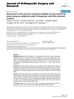
In Fig. 1 the measuring scale is not straight, giving
a pitch error. The size of the error depends on
the distance L of the measured point from the scale
and the angular error 1. For many instruments this Abbe

offset L is not near zero and significant errors can
be made.
The geometry of gage block interferometers includes
two corrections that contribute to the measurement un-
certainty. If the light source is larger than 1 mm in any
direction (a slit for example) a correction must be made.
If the light path is not orthogonal to the surface of the
gage there is also a correction related to cosine errors
called obliquity correction. Comparison of results be-
tween instruments with different geometries is an ade-
quate check on the corrections supplied by the manufac-
turer.
Fig. 1. The Abbe error is the product of the perpendicular distance of the scale from the
measuring point, L, times the sine of the pitch angle error,
⌰
, error = L sin
⌰
.
653
Volume 102, Number 6, November–December 1997
Journal of Research of the National Institute of Standards and Technology
3.7 Artifact Effects
The last major sources of uncertainty are the proper-
ties of the customer artifact. The most important of
these are thermal and geometric. The thermal expansion
of customer artifacts was discussed earlier (Sec. 3.3).
Perhaps the most difficult source of uncertainty to
evaluate is the effect of the test gage geometry on the
calibration. We do not have time, and it is not economi-
cally feasible, to check the detailed geometry of every

artifact we calibrate. Yet we know of many artifact
geometry flaws that can seriously affect a calibration.
We test the diameter of gage balls by repeated com-
parisons with a master ball. Generally, the ball is
measured in a random orientation each time. If the ball
is not perfectly round the comparison measurements
will have an added source of variability as we sample
different diameters of the ball. If the master ball is not
round it will also add to the variability. The check
standard measurement samples this error in each
measurement.
Gage wires can have significant taper, and if we
measure the wire at one point and the customer uses it
at a different point our reported diameter will be wrong
for the customer’s measurement. It is difficult to esti-
mate how much placement error a competent user of the
wire would make, and thus difficult to include such
effects in the uncertainty budget. We have made as-
sumptions on the basis of how well we center the wires
by eye on our equipment.
We calibrate nearly all customer gage blocks by
mechanical comparison to our master gage blocks. The
length of a master gage block is determined by interfer-
ometric measurements. The definition of length for
gage blocks includes the wringing layer between the
block and the platen. When we make a mechanical
comparison between our master block and a test block
we are, in effect, assigning our wringing layer to the test
block. In the last 100 years there have been numerous
studies of the wringing layer that have shown that the

thickness of the layer depends on the block and platen
flatness, the surface finish, the type and amount of fluid
between the surfaces, and even the time the block has
been wrung down. Unfortunately, there is still no way to
predict the wringing layer thickness from auxiliary
measurements. Later we will discuss how we have
analyzed some of our master blocks to obtain a quantita-
tive estimate of the variability.
For interferometric measurements, such as gage
blocks, which involve light reflecting from a surface, we
must make a correction for the phase shift that occurs.
There are several methods to measure this phase shift,
all of which are time consuming. Our studies show that
the phase shift at a surface is reasonably consistent for
any one manufacturer, material, and lapping process, so
that we can assign a “family” phase shift value to each
type and source of gage blocks. The variability in each
family is assumed small. The phase shift for good qual-
ity gage block surfaces generally corresponds to a length
offset of between zero (quartz and glass) and 60 nm
(steel), and depends on both the materials and the
surface finish. Our standard uncertainty, from numerous
studies, is estimated to be less than 10 nm.
Since these effects depend on the type of artifact, we
will postpone further discussion until we examine each
calibration.
3.8 Calculation of Uncertainty
In calculating the uncertainty according to the ISO
Guide [2] and NIST Technical Note 1297 [3], individual
standard uncertainty components are squared and added

together. The square root of this sum is the combined
standard uncertainty. This standard uncertainty is then
multiplied by a coverage factor k. At NIST this coverage
factor is chosen to be 2, representing a confidence level
of approximately 95 %.
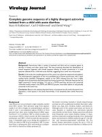
When length-dependent uncertainties of the form
a+bL are squared and then added, the square root is not
of the form a+bL. For example, in one calibration there
are a number of length-dependent and length-indepen-
dent terms:
u
1
= 0.12 ␮m
u
2
= 0.07 ␮m+0.03ϫ10
–6
L
u
3
= 0.08ϫ10
–6
L
u
4
= 0.23ϫ10
–6
L
If we square each of these terms, sum them, and take the
square root we get the lower curve in Fig. 2.

Note that it is not a straight line. For convenience we
would like to preserve the form a+bL in our total uncer-
tainty, we must choose a line to approximate this curve.
In the discussions to follow we chose a length range and
approximate the uncertainty by taking the two end
points on the calculated uncertainty curve and use the
straight line containing those points as the uncertainty.
In this example, the uncertainty for the range
0 to 1 length units would be the line f=a+bL containing
the points (0, 0.14 ␮m ) and (1, 0.28 ␮m).
Using a coverage factor k = 2 we get an expanded
uncertainty U of U = 0.28 ␮m+0.28ϫ10
–6
L for L be-
tween 0 and 1. Most cases do not generate such a large
curvature and the overestimate of the uncertainty in the
mid-range is negligible.
654
Volume 102, Number 6, November–December 1997
Journal of Research of the National Institute of Standards and Technology
3.9 Uncertainty Budgets for Individual
Calibrations
In the remaining sections we discuss the uncertainty
budgets of calibrations performed by the NIST Engi-
neering Metrology Group. For each calibration we list
and discuss the sources of uncertainty using the generic
uncertainty budgetas a guide. At the end of each discus-
sion is a formal uncertainty budget with typical values
and calculated total uncertainty.
Note that we use a number of different calibration

methods for some types of artifacts. The method chosen
depends on the requested accuracy, availability of
master standards, or equipment. We have chosen one
method for each calibration listed below.
Further, many calibrations have uncertainties that are
very sensitive to the size and condition of the artifact.
The uncertainties shown are for “typical” customer
calibrations. The uncertainty for any individual calibra-
tion may differ considerably from the results in this
work because of the quality of the customer gage or
changes in our procedures.
The calibrations discussed are:
Gage blocks (interferometry)
Gage blocks (mechanical comparison)
Gage wires (thread and gear wires) and
cylinders (plug gages)
Ring gages (diameter)
Gage balls (diameter)
Roundness standards (balls, rings, etc.)
Optical flats Indexing tables
Angle blocks
Sieves
The calibration of line scales is discussed in a separate
document [17].
4. Gage Blocks (Interferometry)
The NIST master gage blocks are calibrated by inter-
ferometry using a calibrated HeNe laser as the light
source [18]. The laser is calibrated against an iodine-
stabilized HeNe laser. The frequency of stabilized
lasers has been measured by a number of researchers

and the current consensus values of different stabilized
frequencies are published by the International Bureau of
Weights and Measures [12]. Our secondary stabilized
lasers are calibrated against the iodine-stabilized laser
using a number of different frequencies.
4.1 Master Gage Calibration
This calibration does not use master reference gages.
Fig. 2. The standard uncertainty of a gage block as a function of length (a) and the linear
approximation (b).
655
Volume 102, Number 6, November–December 1997
Journal of Research of the National Institute of Standards and Technology
4.2 Long Term Reproducibility
The NIST master gage blocks are not used until they
have been measured at least 10 times overa3yearspan.
This is the minimum number of wrings we think will
give a reasonable estimate of the reproducibility and
stability of the block. Nearly all of the current master
blocks have considerably more data than this minimum,
with some steel blocks being measured more than
50 times over the last 40 years. These data provide an
excellent estimate of reproducibility. In the long term,
we have performed calibrations with many different
technicians, multiple calibrations of environmental
sensors, different light sources, and even different inter-
ferometers.
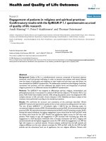
As expected, the reproducibility is strongly length
dependent, the major variability being caused by
thermal properties of the blocks and measurement
apparatus. The data do not, however, fall on a smooth

line. The standard deviation data from our calibration
history is shown in Fig. 3.
There are some blocks, particularly long blocks,
which seem to have more or less variability than the
trend would predict. These exceptions are usually
caused by poor parallelism, flatness or surface finish
of the blocks. Ignoring these exceptions the standard
deviation for each length follows the approximate
formula:
u(rep) = 0.009 ␮m+0.08ϫ10
–6
L (NIST Masters)
(4)
For interferometry on customer blocks the reproduci-
bility is worse because there are fewer measurements.
The numbers above represent the uncertainty of the
mean of 10 to 50 wrings of our master blocks. Customer
calibrations are limited to 3 wrings because of time and
financial constraints. The standard deviation of the
mean of n measurements is the standard deviation of the
n measurements divided by the square root of n.Wecan
relate the standard deviation of the mean of 3 wrings to
the standard deviations from our master block history
through the square root of the ratio of customer rings (3)
to master block measurements (10 to 50). We will use 20
as the average number of wrings for NIST master
blocks. The uncertainty of 3 wrings is then approxi-
mately 2.5 times that for the NIST master blocks. The
standard uncertainty for 3 wrings is
u(rep) = 0.022 ␮m+0.20ϫ10

–6
L (3 wrings).
(5)
4.3 Thermal Expansion
4.3.1 Thermometer Calibration The thermo-
meters used for the calibrations have been changed over
the years and their history samples multiple calibrations
of each thermometer. Thus, the master block historical
data already samples the variability from the thermome-
ter calibration.
Thermistor thermometers are used for the calibration
of customer blocks up to 100 mm in length. As dis-
cussed earlier [(see eq. 2)] we will take the uncertainty
Fig. 3. Standard deviations for interferometric calibration of NIST master gage blocks of different length as
obtained over a period of 25 years.
656
Volume 102, Number 6, November–December 1997
Journal of Research of the National Institute of Standards and Technology
of the thermistor thermometers tobe 0.01 ЊC. For longer
blocks, a more accurate system consisting of a platinum
SPRT (Standard Platinum Resistance Thermometer) as
a reference and thermocouples is used.
4.3.2 Coefficient of Thermal Expansion (CTE)
The CTE of each of our blocks over 25 mm in length
has been measured, leaving a very small standard uncer-
tainty estimated to be 0.05ϫ10
–6
/ЊC. Since our
measurements are always within Ϯ0.1 ЊCof20ЊC, the
uncertainty in length is taken to be 0.005ϫ10

–6
L.
4.3.3 Thermal Gradients The long block tem-
perature is measured every 100 mm, reducing the
effects of thermal gradients to a negligible level.
The gradients between the thermometer and test
blocks in the short block interferometer (up to 100 mm)
are small because the entire measurement space is in a
metal enclosure. The gradients between the thermome-
ter in the center of the platen and any block are less than
0.005 ЊC. Assuming a rectangular distribution with a
half-width 0.005 ЊC, we obtain a standard uncertainty of
0.003 ЊC in temperature. For steel gage blocks
(CTE = 11.5 ␮m/(m иЊC) ), the standard uncertainty in
length is 0.003ϫ10
–6
L. For other materials the uncer-
tainty is less.
4.4 Elastic Deformation
We measure blocks oriented vertically, as specified in
the ANSI/ASME B89.1.9 Gage Block Standard [19].
For customers who need the length of long blocks in the
horizontal orientation, a correction factor is used. This
correction for self loading is proportional to the square
of the length, and is very small compared to other
effects. For 500 mm blocks the correction is only about
25 nm, and the uncertainty depends on the uncertainty
in the elastic modulus of the gage block material. Nearly
all long blocks are made of steel, and the variations
in elastic modulus for gage block steels is only a few

percent. The standard uncertainty in the correction is
estimated to be less than 2 nm, a negligible addition to
the uncertainty budget.
4.5 Scale Calibration
The laser is calibrated against a well characterized
iodine-stabilized laser. We estimate the relative standard
uncertainty in the frequency from this calibration to
be less than 10
–8
, which is negligible for gage block
calibrations.
The Edle´n equation for the index of refraction of air,
n, has a relative standard uncertainty of 3ϫ10
–8
.
Customer calibrations are made under a single
environmental sensor calibration cycle and the uncer-
tainty from these sources must be estimated. We check
our pressure sensors against a barometric pressure
standard maintained by the NIST Pressure Group.
Multiple comparisons lead us to estimate the standard
uncertainty of our pressure gages is 8 Pa. The air
temperature measurement has a standard uncertainty of
about 0.015 ЊC, as discussed previously. By comparing
several hygrometers we estimate that the standard uncer-
tainty of the relative humidity is about 3 %.
The gage block historical data contains measurements
made with a number of sources including elemental
discharge lamps (cadmium, helium, krypton) and
several calibrated lasers. The historical data, therefore,

contains an adequate sampling of the light source
frequency uncertainty.
4.6 Instrument Geometry
The obliquity and slit corrections provided by the
manufacturers are used for all of our interferometers.
We have tested these corrections by measuring the same
blocks in all of the interferometers and have found no
measurable discrepancies. Measuring blocks in interfer-
ometers of different geometries could also be used to
find the corrections. For example, our Koesters type
interferometer has no obliquity correction when prop-
erly aligned, and the slit is accessible for measurement.
Thus, the correction can be calculated. The Hilger inter-
ferometer slits cannot be measured except by disassem-
bly, but the corrections can be found by comparison of
measurements with the Koesters interferometer.
The only geometry errors, other than those discussed
above, are due to the platen flatness. Each platen is
examined and is not used unless it is flat to 50 nm over
the entire 150 mm diameter. Since the gage block mea-
surement is made over less than 25 mm of the surface,
the local flatness is quite good. In addition, the measure-
ment history of the master blocks has data from many
platens and multiple positions on each platen, so the
variability from the platen flatness is sampled in the
data.
4.7 Artifact Geometry
The phase change that light undergoes on reflection
depends on the surface finish and the electromagnetic
properties of the block material. We assume that every

block from a single manufacturer of the same material
has the same surface finish and material, and therefore
gives rise to the same phase change. We have restricted
our master blocks to a few manufacturers and materials
to reduce the work needed to characterize the phase
change. Samples of each material and manufacturer are
measured by the slave block method [4], and these
results are used for all blocks of similar material and the
same manufacturer.
657
Volume 102, Number 6, November–December 1997
Journal of Research of the National Institute of Standards and Technology
In the slave block method, an auxiliary block, called
the slave block, is used to help find the phase shift
difference between a block and a platen. The method
consists of two steps, shown schematically in Figs. 4
and 5.
The interferometric length L
test
includes the mechani-
cal length, the wringing film thickness, and the phase
change at each surface.
Step 1. The test and slave blocks are wrung down to
the same platen and measured independently. The two
lengths measured consist of the mechanical length of the
block, the wringing film, and the phase changes at the
top of the block and platen, as in Fig. 4.
The general formula for the measured length of a
wrung block is:
L

test
= L
mechanical
+L
wring
+L
platen phase
–L
block phase
. (6)
For the test and slave blocks the formulas are
L
test
= L
t
+L
t,w
+(
␾
platen
–
␾
test
) (7)
L
slave
= L
s
+L
s,w

+(
␾
platen
–
␾
slave
) (8)
where L
t
, L
t,w
, L
s
,andL
s,w
are defined in Fig. 4.
Step 2. Either the slave block or both blocks are taken
off the platen, cleaned, and rewrung as a stack on the
platen. The length of the stack measured is:
L
test+slave
= L
t
+L
s
+L
t,w
+L
s,w
+(

␾
platen
–
␾
slave
). (9)
If this result is subtracted from the sum of the two
previous measurements, we find that
L
test+slave
–L
test
–L
slave
=(
␾
test
–
␾
platen
). (10)
The weakness of this method is the uncertainty of the
measurements. The standard uncertainty of one
measurement of a wrung gage block is about 0.030 ␮m
(from the long term reproducibility of our master block
calibrations). Since the phase measurement depends on
three measurements, the phase measurement has a
standard uncertainty of about ͙3 times the uncertainty
of one measurement, or about 0.040 ␮m. Since the
phase difference between block and platen is generally

corresponds to a length of about 0.020 ␮m, the un-
certainty is larger than the effect. To reduce the uncer-
tainty, a large number of measurements must be made,
generally around 50. This is, of course, very time
consuming.
For our master blocks, using the average number of
slave block measurements gives an estimate of
0.006 ␮m for the standard uncertainty due to the phase
correction.
We restrict our calibration service to small (8 to 10
block) audit sets for customers who do interferometry.
These audit sets are used as checks on the customer
measurement process, and to assure that the uncertainty
is low we restrict the blocks to those from manufacturers
for which we have adequate phase-correction data. The
uncertainty is, therefore, the same as for our own master
blocks. On the rare occasions that we measure blocks of
unknown phase, the uncertainty is very dependent on
the procedure used, and is outside the scope of this
paper.
If the gage block is not flat and parallel, the fringes
will be slightly curved and the position on the block
Fig. 4. Diagram showing the phase shift
␾
on reflection makes
the light appear to have reflected from a surface slightly above the
physical metal surface.
Fig. 5. Schematic depiction of the measurements for determining the
phase shift difference between a block and platen by the slave block
method.

658
Volume 102, Number 6, November–December 1997
Journal of Research of the National Institute of Standards and Technology
where the fringe fraction is measured becomes impor-
tant. For our measurements we attempt to read the
fringe fraction as close to the gage point as possible.
However, using just the eye, this is probably uncertain to
1 mm to 2 mm. Since most blocks we measure are flat
and parallel to 0.050 ␮m over the entire surface, the
error is small. If the block is 9 mm wide and the flatness/
parallelism is 0.050 ␮m then a 1 mm error in the gage
point produces a length error of about 0.005 ␮m. For
customer blocks this is reduced somewhat because three
measurements are made, but since the readings are
made by the same person operator bias is possible. We
use a standard uncertainty of 0.003 ␮m to account for
this possibility. Our master blocks are measured over
many years by different technicians and the variability
from operator effects are sampled in the historical data.
5. Gage Blocks (Mechanical Comparison)
Most customer calibrations are made by mechanical
comparison to master gage blocks calibrated on a regu-
lar basis by interferometry. The comparison process
compares each gage block with two NIST master blocks
of the same nominal size [20]. We have one steel and one
chrome carbide master block for each standard size. The
customer block length is derived from the known length
of the NIST master made of the same material to
avoid problems associated with deformation corrections.
4.8 Summary

Tables 3 and 4 show the uncertainty budgets for inter-
ferometric calibration of our master reference blocks
and customer submitted blocks. Using a coverage factor
of k = 2 we obtain the expanded uncertainty U of our
interferometer gage block calibrations for our master
gage blocks as U = 0.022 ␮m+0.16ϫ10
–6
L.
The uncertainty budget for customer gage block
calibrations (three wrings) is only slightly different.
The reproducibility uncertainty is larger because of
fewer measurements and because the thermal expansion
coefficient has not been measured on customer blocks.
Using a coverage factor of k=2 we obtain an expanded
uncertainty U for customer calibrations (three wrings)
of U = 0.05 ␮m+0.4ϫ10
–6
L.
Deformation corrections are needed for tungsten
carbide blocks and we assign higher uncertainties than
those described below.
In the discussion below we group gage blocks into
three groups, each with slightly different uncertainty
statements. Sizes over 100 mm are measured on differ-
ent instruments than those 100 mm or less, and have
different measurement procedures. Thus they form a
distinct process and are handled separately. Blocks
under 1 mm are measured on the same equipment as
those between 1 mm and 100 mm, but the blocks have
Table 3. Uncertainty budget for NIST master gage blocks

Source of uncertainty Standard uncertainty (k =1)
1. Master gage calibration N/A
2. Long term reproducibility 0.009 ␮m+0.08ϫ10
–6
L
3. Thermometer calibration N/A
4. CTE 0.005ϫ10
–6
L
5. Thermal gradients 0.030ϫ10
–6
L up to L=0.1 m
6. Elastic deformation Negligible
7. Scale calibration 0.003ϫ10
–6
L
8. Instrument geometry Negligible
9. Artifact geometry—phase correction 0.006 ␮m
Table 4. Uncertainty budget for NIST customer gage blocks measured by interferometry
Source of uncertainty Standard uncertainty (k =1)
1. Master gage calibration N/A
2. Long term reproducibility 0.022 ␮m+0.2ϫ10
–6
L
3. Thermometer calibration N/A
4. CTE 0.060ϫ10
–6
L
5. Thermal gradients 0.030ϫ10
–6

L up to L=0.1 m
6. Elastic deformation Negligible
7. Scale calibration 0.003ϫ10
–6
L
8. Instrument geometry Negligible
9. Artifact geometry—phase correction 0.006 ␮m
10. Artifact geometry—gage point position 0.003 ␮m
659
Volume 102, Number 6, November–December 1997
Journal of Research of the National Institute of Standards and Technology
different characteristics and are considered here as a
separate process. The major difference is that thin
blocks are generally not very flat, and this leads to an
extra uncertainty component. They are also so thin that
length-dependent sources of uncertainty are negligible.
5.1 Master Gage Calibration
From the previous analysis (see Sec. 4.8) the standard
uncertainty u of the length of the NIST master blocks is
u = 0.011 ␮m+0.08ϫ10
–6
L. Of course, some blocks
have a longer measurement history than others, but for
this discussion we use the average. We use the actual
value for each master block to calculate the uncertainty
reported for the customer block. Thus, numbers gener-
ated in this discussion only approximate those in an
actual report.
5.2 Long Term Reproducibility
We use two NIST master gage blocks in every

calibration, one steel and the other chrome carbide.
When the customer block is steel or ceramic, the steel
block length is the master (restraint in the data analysis).
When the customer block is chrome or tungsten
carbide, the chrome carbide block is the master. The
difference between the two NIST blocks is a control
parameter (check standard).
The check standard data are used to estimate the long
term reproducibility of the comparison process. The
two NIST blocks are of different materials so the
measurements have some variability due to contact force
variations (deformation) and temperature variations
(differential thermal expansion). Customer
calibrations, which compare like materials, are less
susceptible to these sources of variability. Thus, using
the check standard data could produce an overestimate
of the reproducibility. We do have some size ranges
where both of the NIST master blocks are steel, and the
variability in these calibrations has been compared to
the variability among similar sizes where we have
masters of different material. We have found no sig-
nificant difference, and thus consider our use of the
check standard data as a valid estimate of the long term
reproducibility of the system.
The standard uncertainty derived from our control
data is, as expected, a smooth curve that rises slowly
with the length of the blocks. For mechanical compari-
sons we pool the control data for similar sizes to obtain
the long term reproducibility. We justify this grouping
by examining the sources of uncertainty. The inter-

ferometry data are not grouped because the surface
finish, material composition, flatness, and thermal
properties affect the measured length. The surface
finish and material composition affect the phase shift
and the flatness affects the wringing layer between the
block and platen. The mechanical comparisons are not
affected by any of these factors. The major remaining
factor is the thermal expansion. We therefore pool the
control data for similar size blocks. Each group has
about 20 sizes, until the block lengths become greater
than 25 mm. For these blocks the thermal differences
are very small. For longer blocks, the temperature ef-
fects become dominant and each size represents a
slightly different process; therefore the data are not
combined.
For this analysis we break down the reproducibility
into three regimes: thin blocks (less than 1 mm), long
blocks (>100 mm), and the intermediate range that con-
tains most of the blocks we measure. This is a natural
breakdown because blocks Յ100 mm are measured
with a different type of comparator and a different com-
parison scheme than are used for blocks >100 mm. A fit
to the historical data produces an uncertainty com-
ponent (standard deviation) for each group as shown in
Table 5.
5.3 Thermal Expansion
5.3.1 Thermometer Calibration For compari-
son measurements of similar materials, the thermome-
ter calibration is not very important since the tempera-
ture error is the same for both blocks.

5.3.2 Coefficient of Thermal Expansion The
variation in the CTE for similar gage block materials is
generally smaller than the Ϯ1ϫ10
–6
/ЊC allowed by the
ISO and ANSI gage block standards. From the variation
of our own steel master blocks, we estimate the standard
uncertainty of the CTE to be 0.4ϫ10
–6
/ЊC. Since we do
not measure gage blocks if the temperature is more than
0.2 ЊC from 20 ЊC, the length-standard uncertainty is
0.08ϫ10
–6
L. For long blocks (L>100 mm) we do not
perform measurements if the temperature is more than
0.1 ЊC from 20 ЊC, reducing the standard uncertainty to
0.04ϫ10
–6
L.
5.3.3 Thermal Gradients The uncertainty due to
thermal gradients is important. For the short block
comparator temperature differences up to Ϯ0.030 ЊC
have been measured between blocks positioned on the
Table 5. Standard uncertainty for length of NIST master gage
blocks
Type of block Standard uncertainty
Thin (<1 mm) 0.008 ␮m
Intermediate (1 mm to 100 mm) 0.004 ␮m+0.12ϫ10
–6

L
Long (>100 mm) 0.020 ␮m+0.03ϫ10
–6
L
660
Volume 102, Number 6, November–December 1997
Journal of Research of the National Institute of Standards and Technology
comparator platen. Assuming a rectangular distribution
we get a standard temperature uncertainty of 0.017 ЊC.
The temperature difference affects the entire length of
the block, and the length standard uncertainty is the
temperature difference times the CTE times the length
of the block. Thus for steel it would be 0.20ϫ10
–6
L
and for chrome carbide 0.14ϫ10
–6
L. For our simpli-
fied discussion here we use the average value of
0.17ϫ10
–6
L.
The precautions used for long block comparisons
result in much smaller temperature differences between
blocks, 0.010 ЊC and less. Using this number as the
half-width of a rectangular distribution we get a
standard temperature uncertainty of 0.006 ЊC. Since
nearly all blocks over 100 mm are steel we find the
standard uncertainty component to be 0.07ϫ10
–6

L.
5.4 Elastic Deformation
Since most of our calibrations compare blocks of the
same material, the elastic deformation corrections are
not needed. There is, in theory, a small variability in the
elastic modulus of blocks of the same material. We have
not made systematic measurements of this factor. Our
current comparators have nearly flat contacts, from
wear, and we calculate that the total deformations are
less than 0.05 ␮m. If we assume that the elastic proper-
ties of gage blocks of the same material vary byless than
5 % we get a standard uncertainty of 0.002 ␮m. We have
tested ceramic blocks and found that the deformation is
the same as steel for our conditions.
For materials other than steel, chrome carbide, and
ceramic (zirconia), we must make penetration cor-
rections. Unfortunately, we have discovered that the
diamond styli wear very quickly and the number of
measurements which can be made without measurable
changes in the contact geometry is unknown. From our
historical data, we know that after 5000 blocks, both of
our comparators had flat contacts. We currently add an
extra component of uncertainty for measurements
of blocks for which we do not have master blocks of
matching materials.
5.5 Scale Calibration
The gage block comparators are two point-contact
devices, the block being held up by an anvil. The length
scale is provided by a calibrated linear variable differen-
tial transformer (LVDT). The LVDT is calibrated in

situ using a set of gage blocks. The blocks have nominal
lengths from 0.1 in to 0.100100 in with 0.000010 in
steps. The blocks are placed between the contacts of
the gage block comparator in a drift eliminating
sequence; a total of 44 measurements, four for each
block, are made. The known differences in the lengths
of the blocks are compared with the measured voltages
and a least-squares fit is made to determine the slope
(length/voltage) of the sensor. This calibration is done
weekly and the slope is recorded. The standard deviation
of this slope history is taken as the standard uncertainty
of the sensor calibration, i.e., the variability of the scale
magnification. Over the last few years the relative
standard uncertainty has been approximately 0.6 %.
Since the largest difference between the customer and
master block is 0.4 ␮m (from customer histories), the
standard uncertainty due to the scale magnification is
0.006ϫ0.4 ␮m = 0.0024 ␮m.
The long block comparator has older electronics and
has larger variability in its scale calibration. This vari-
ability is estimated to be 1 %. The long blocks also have
a much greater range of values, particularly blocks man-
ufactured before the redefinition of the in in 1959.
When the in was redefined its value changed relative to
the old in by 2ϫ10
–6
, making the length value of all
existing blocks larger. The difference between our mas-
ter blocks and customer blocks can be as large as 2 ␮m,
and the relative standard uncertainty of 1 % in the scale

linearity yields a standard uncertainty of 0.020 ␮m.
5.6 Instrument Geometry
If the measurements are comparisons between blocks
with perfectly flat and parallel gaging surfaces, the
uncertainties resulting from misalignment of the
contacts and anvil are negligible. Unfortunately, the
artifacts are not perfect. The interaction of the surface
flatness and the contact alignment is a small source of
variability in the measurements, particularly for thin
blocks. Thin blocks are often warped, and can be out of
flat by 10 ␮m, or more. If the contacts are not aligned
exactly or the contacts are not spherical, the contact
points with the block will not be perpendicular to the
block. Thus the measurement will be slightly larger than
the true thickness of the block. We have made multiple
measurements on such blocks, rotating the block so that
the angle between the block surface and the contact line
varies as much as possible. From these variations we
find that for thin blocks (<1 mm), the standard uncer-
tainty is 0.010 ␮m.
5.7 Artifact Geometry
The definition of length for a gage block is the
perpendicular distance from the gage point on top to the
corresponding point on the flat surface (platen) to which
it is wrung. If the platen and gage block are perfectly flat
this distance would be the mechanical distance from the
gage points on the top and bottom of the block plus the
thickness of the wringing layer. If the customer block
also was perfectly flat, the difference in the defined
length (from interferometry) and the mechanical length

(from the two-point comparison) would be the same.
661
Volume 102, Number 6, November–December 1997
Journal of Research of the National Institute of Standards and Technology
The customer block and the NIST master are not, of
course, perfectly flat. This leaves the possibility that the
calibration will be in error because the comparison
process, in effect, assigns the bottom geometry and
wringing film of the NIST master to the customer block.
We have attempted to estimate this error from our
history of the measurements of the 2 mm series of
metric blocks. All of these blocks are steel and from the
same manufacturer, eliminating the complications of
the interferometric phase correction. If there is no error
due to surface flatness, the length difference found by
interferometry and by mechanical comparisons should
be equal.
Analyzing this data is difficult. Since eitheror both of
the blocks could be the cause of an offset, the average
offset seen in the data is expected to be zero. The
signature of the effect is a wider distribution of the data
than expected from the individual uncertainties in the
interferometry and comparison process.
For each size the difference between interferometric
and mechanical length is a measure of the bias caused
by the geometry of the gaging surfaces of the blocks.
This bias is calculated from the formula
B =(L1
int
–L2

int
)–(L1
mech
–L2
mech
) (11)
where B is the bias, L1
int
and L2
int
are the lengths of
blocks 1 and 2 measured by interferometry, and L1
mech
and L2
mech
the lengths of blocks 1 and 2 measured by
mechanical comparison. Because the geometry effects
can be of either sign, the average bias over a number of
blocks is zero. There is, fortunately, more useful infor-
mation in the variation of the bias because it is made up
of three components: the variations in the interfero-
metric length, the mechanical length, and the geometry
effects. The variation in the interferometric and
mechanical length differences can be obtained from the
interferometric history and the check standard data,
respectively. Assuming that all of the distributions are
normal, the measured standard deviations are related
by:
S
2

bias
= S
2
int
= S
2
mech
= S
2
geom
(12)
Our data for the 2 mm series is shown below. The
numbers given are somewhat different than the tables
show for typical calibrations for these sizes. The 2 mm
series is not very popular with our customers, and since
we do few calibrations in these sizes there are fewer
interferometric measurements of the masters and fewer
check standard data. We analyzed 58 pairs of blocks
from the 2 mm series blocks and obtained estimated
standard deviations of 0.017 ␮m for the bias, 0.014 ␮m
for the interferometric differences and 0.005 ␮m for the
mechanical differences. This gives 0.008 ␮masthe
standard uncertainty in gage length due to the block
surface geometry.
Another way to estimate this effect is to measure the
blocks in two orientations, with each end wrung to the
platen in turn. We have not made a systematic study with
this method but we do have some data gathered in con-
junction with international interlaboratory tests. This
data suggest that the effect is small for blocks under a

few millimeters, but becomes larger for longer blocks.
This suggests that the thin blocks deform to the shape of
the plated when wrung, but longer blocks are stiff
enough to resist the deformation. Since both of the
surfaces are made with the same lapping process, this
estimate may be somewhat smaller than the general
case. This effect is potentially a major source of uncer-
tainty and we plan further tests in the future.
5.8 Summary
The uncertainty budget for gage block calibration by
mechanical comparison is shown in Table 6. The
expanded uncertainty (coverage factor k = 2) for each
type of calibration is
Thin Blocks (L<1mm) U=0.040␮m
Gage Blocks (1mm to 100mm) U=0.030␮m+0.35ϫ10
–6
L
Long Blocks (100mm<LՅ 500mm) U=0.055␮m+0.20ϫ10
–6
L.
For long blocks with known thermal expansion coeffi-
cients, the uncertainty is smaller than stated above.
Table 6. Uncertainty budget for NIST customer gage blocks measured by mechanical comparison
Source of uncertainty Standard uncertainty (k =1)
Thins (<1 mm) 1 mm to 100 mm over 100 mm
1. Master gage cal. 0.012 ␮m 0.012 ␮m+0.08ϫ10
–6
L 0.012 ␮m+0.08ϫ10
–6
L

2. Reproducibility 0.008 ␮m 0.004 ␮m+0.12ϫ10
–6
L 0.020 ␮m+0.03ϫ10
–6
L
3a. Thermometer cal. negligible negligible negligible
3b. CTE 0.08ϫ10
–6
L 0.08ϫ10
–6
L 0.04ϫ10
–6
L
3c. Thermal Gradients 0.17ϫ10
–6
L 0.17ϫ10
–6
L 0.07ϫ10
–6
L
4. Elastic Deformation 0.002 ␮m 0.002 ␮m 0.002 ␮m
5. Scale Calibration 0.002 ␮m 0.002 ␮m 0.020 ␮m
6. Instrument Geometry 0.010 ␮m 0.002 ␮m 0.002 ␮m
7. Artifact Geometry 0.008 ␮m 0.008 ␮m 0.008 ␮m
662
Volume 102, Number 6, November–December 1997
Journal of Research of the National Institute of Standards and Technology
6. Gage Wires (Thread and Gear Wires)
and Cylinders (Plug Gages)
Customer wires are calibrated by comparison to

master wires using several different micrometers. Most
of the micrometers have flat parallel contacts, but
cylinder contacts are occasionally used. The sensors
are mechanical twisted thread comparators, electronic
LVDTs, and interferometers.
For gage wires, gear wires, and cylinders we report
the undeformed diameter. If the wire is a thread wire the
proper deformation is calculated and the corrected
(deformed) diameter is reported.
The master wires and cylinders have been calibrated
by a variety of methods over the last 20 years:
1. Large cylinders are usually calibrated by compari-
son to gage blocks using a micrometer with flat
contacts.
2. A second device uses two optical flats with gage
blocks wrung in the center as anvils. The upper
flat has a fixture that allows it to be set at any
height and adjusted nearly parallel to the bottom
flat. The wire or cylinder is placed between the
two gage blocks (wrung to the flats) and the top
flat is adjusted to form a slight wedge. This wedge
forms a Fizeau interferometer and the distance be-
tween the two flats is determined by multicolor
interferometry. The cylinder or wire diameter is
the distance between the flats minus the lengths of
the gage blocks.
3. A third device consists of a moving flat anvil and
a fixed cylindrical anvil. A displacement interfer-
ometer measures the motion of the moving anvil.
4. Large diameter cylinders can be compared to gage

blocks using a gage block comparator.
6.1 Master Artifact Calibration
The master wires are measured by a number of
methods including interferometry and comparison to
gage blocks. We will take the uncertainty in the wires
and cylinders as the standard deviation of the master
calibrations over the last 20 years. Because of the
number of different measurement methods, eachwith its
own characteristic systematic errors, and the long period
of time involved, we assume that all of the pertinent
uncertainty sources have been sampled. The standard
deviation derived from 168 degrees of freedom is
0.065 ␮m.
6.2 Long Term Reproducibility
We use check standards extensively in our wire calibra-
tions, which produces a record of the long term repro-
ducibility of the calibration. A typical data set is shown
in Fig. 6.
While we do not use check standards for every size
and type of wire, the difference in the measurement
process for similar sizes is negligible. From our
long-term measurement data we find the standard
uncertainty for reproducibility (one standard deviation,
300 degrees of freedom) is u = 0.025 ␮m.
6.3 Thermal Expansion
6.3.1 Thermometer Calibration Since all cus-
tomer calibrations are done by mechanical comparison
the uncertainty due to the thermometer calibration is
negligible.
6.3.2 Coefficient of Thermal Expansion Nearly

all wires are steel, although some cylinders are made of
other materials. Since we measure within 0.2 ЊCof
20 ЊC, if we assume a rectangular distribution and we
we know the CTE to about 10 %, we get a differential
expansion uncertainty of 0.01ϫ10
–6
L.
6.3.3 Thermal Gradients We have found tem-
perature differences up to Ϯ0.030 ЊC in the calibration
area of our comparators, and using 0.030 ЊC as the half-
width of a rectangular distribution we get a standard
temperature uncertainty of 0.017 ЊC, which leads to a
length standard uncertainty of 0.017ϫ10
–6
L.
6.4 Elastic Deformation
The elastic deformations under the measurement con-
ditions called out in the screw thread standard [10] are
very large, 0.5 ␮mto1␮m. Because we do not perform
master wire calibrations at standard conditions we must
make corrections for the actual deformation during the
measurement to get the undeformed diameter, and then
apply a further correction to obtain the diameter at the
standard conditions. When both deformation corrections
are applied to the master wire diameter, the comparator
process automatically yields the correct standard diame-
ter of the customer wires.
Our corrections are calculated according to formulas
derived at Commonwealth Scientific and Industrial Re-
search Organization (CSIRO), and have been checked

experimentally. There is no measurable bias between the
calculated and measured deformations when the elastic
modulus of the material is well known. Unfortunately,
there is a significant variation in the reported elastic
663
Volume 102, Number 6, November–December 1997
Journal of Research of the National Institute of Standards and Technology
modulus for most common gage materials. An examina-
tion of a number of handbooks for the elastic moduli
gives a relative standard deviation of 3 % for hardened
steel, and 5 % for tungsten carbide.
If we examine a typical case for thread wires (40
pitch) we have the corrections shown in Fig. 7. Line
contacts have small deformations and point contacts
have large deformations. For a typical wire calibration
the deformation at the micrometer zero, Dz,isaline
contact with a deformation of 0.003 ␮m. The deforma-
tion of the wire at the micrometer flat contact , Dw /s,
is also a line contact with a value of 0.003 ␮m. The
contact between the micrometer cylinder anvil and wire
is a point contact, Dw/a, which has the much larger
deformation of 0.800 ␮m.
Once these corrections are made the wire measure-
ment is the undeformed diameter. To bring the reported
diameter to the defined diameter (deformed at ASME
B1 conditions) a further correction of 1.6 ␮m must be
made. The corrections are thus from a slightly deformed
diameter, as measured, to the undeformed diameter, and
from the undeformed diameter to the standard (B1)
deformed diameter. Since all of the corrections use the

same formula, which we have assumed is correct, the
only uncertainty is in the difference between the two
corrections. In our example this is 0.8 ␮m.
Nearly all gage wires are made of steel. If we take the
elastic modulus distribution of steel to be rectangular
with a half-width of 3 % and apply it to this differential
correction, we get a standard uncertainty of 0.013 ␮m.
6.5 Scale Calibration
The comparator scales are calibrated with gage
blocks. Since several different comparators are used,
each calibrated independently with different gage
blocks, the check standard data adequately samples the
variability in sensor calibration.
6.6 Instrument Geometry
When wires and cylinders are calibrated by compari-
son, the instrument geometry is the same for both mea-
surements and thus any systematic effects are the same.
Since the difference between the measurements is used
for the calibration, the effects cancel.
6.7 Artifact Geometry
If the cylinder is not perfectly round, each time a
different diameter is measured the answer will be differ-
ent. We measure each wire or cylinder multiple times,
changing the orientation each time. If the geometry of
Fig. 6. Check standard data for seven calibrations of a set of thread wires.
Fig. 7. Schematic depiction of the measurement of the wire/spindle
and spindle/anvil contacts are line contacts and involve small defor-
mations. The wire/anvil contactis a pointcontact and thedeformation
is large.
664

Volume 102, Number 6, November–December 1997
Journal of Research of the National Institute of Standards and Technology
the wire is very bad this variation in the readings
will cause the calibration to fail the control test for
repeatability. If not, the wire will pass and the uncer-
tainty assigned will be from the check standard data,
i.e., the check standard wires. Since we pool check
standard data from a number of similar size wires, the
check standard data includes the effects of “average”
roundness.
If the customer wire is significantly more out of
round than our check standard the calibration will fail
the repeatability test. In these cases we increase the
reported uncertainty. For customers who need the
highest accuracy, we measure the roundness as part of
the calibration or make measurements only along one
marked diameter. The customer then makes measure-
ments using the same diameter.
Wires and cylinders can also be tapered. Since we
measure the wires in the middle, but fixture the wires by
hand, there is some uncertainty in the position of the
measurement. According to the thread wire standard,
wires must be tapered less than 0.254 ␮m (10 ␮in) over
the central 25 mm (1 in) of their length. Most of the
wires we calibrate are master wires and are much better
than this limit. Since the fixturing error is less than a
few millimeters, the resultant uncertainty in diameter is
small. As an estimate we assume the central 25 mm of
the wire has a possible diameter change of 0.1 ␮m,
giving a possible diameter change of 0.008 ␮m for an

assumed 2 mm fixturing shift.
6.8 Summary
Table 7 shows the uncertainty budget for wire and
cylinder calibrations. We combine the standard un-
certainties and use a coverage factor of k = 2 to obtain
the expanded uncertainty U for wires up to 25 mm
in diameter of U = 0.14 ␮m+0.03ϫ10
–6
L.
The cylinder calibrations are done with little or no
deformation and therefore the last uncertainty source,
elastic deformation, is negligible. The change is not,
however, large enough to change the uncertainty in the
second decimal digit.
7. Ring Gages (Diameter <100 mm)
Ring gages are measured by comparison to one or
more gage block stacks. Most ring gages have a marked
diameter and this particular diameter is the only
reported value.
7.1 Master Artifact Calibration
Ring gages, in general, do not come in sets of
standardized sizes. Because of this we cannot have
master ring gages. Instead we calibrate ring gages by
comparison to a stack of gage blocks wrung to a preci-
sion square. A gage block stack is prepared the same
length as the nominal ring diameter. This stack is wrung
to a precision square and a 5 mm block is wrung on top
so that about 10 mm of the block extend beyond the end
of the stack, as shown in Fig. 8. This extended surface
of the top block and the surface of the square forms an

internal length to compare with the ring.
The square is longer and wider than the gage block
stack so that the fringe fractions between the surface of
the square and the top of the gage block stack are clearly
visible. The quality of the wring can be seen by examin-
ing the fringes. If the fringes on the block stack and
square are parallel and straight the wring is good.
Fig. 8. Schematic depiction of the use of a gage block stack for use
as a master gage for ring gage calibration.
Table 7. Uncertainty budget for NIST customer gage wires and cylinders measured by mechanical comparison
Source of uncertainty Standard uncertainty (k =1)
1. Master gage calibration 0.065 ␮m
2. Long term reproducibility 0.025 ␮m
3a. Thermometer calibration Negligible
3b. CTE 0.01ϫ10
–6
L
3c. Thermal gradients 0.017ϫ10
–6
L
4. Elastic deformation 0.013 ␮m
5. Scale calibration N/A
6. Instrument geometry N/A
7. Artifact geometry 0.008 ␮m
665
Volume 102, Number 6, November–December 1997
Journal of Research of the National Institute of Standards and Technology
Each stack is measured by multicolor interferometry
to give the highest possible accuracy. The gap is the
difference between the measured length of the top block

and the length of the entire stack. Since the length of the
top block is measured on the square, there is no phase
correction needed, reducing the uncertainty. As an
estimate we use the uncertainty of customer block
calibrations without the phase correction uncertainty.
Since the gap is the difference of two measurements
the total uncertainty is the root-sum-square of two
measurements. The standard uncertainty is
0.038 ␮m+0.2ϫ10
–6
L.
7.2 Long Term Reproducibility
The ring gages we calibrate come in a large variety of
sizes and it is impractical to have master ring gages and
check standards. We do not calibrate enough rings of
any one size to generate statistically significant data. As
an alternative, we use data from our repeat customers
with enough independent measurements on the same
gages to estimate our long term reproducibility.
Measurements on four gages from one customer over the
last 20 years show a standard deviation of 0.025 ␮m.
7.3 Thermal Expansion
7.3.1 Thermometer Calibration The ther-
mometer calibration affects the length of the master
stack, but this effect has been included in the uncer-
tainty of the stack (master).
7.3.2 Coefficient of Thermal Expansion We
choose gage blocks of the same material as the customer
gage to make the master gage block stack. This reduces
the differential expansion coefficient. By using similar

materials as test and master gage the standard uncer-
tainty of the differential thermal expansion coefficient is
0.6ϫ10
–6
/ЊC and all of the measurements are made
within 0.2 ЊCof20ЊC. This uncertainty in thermal
expansion coefficient gives a length standard uncer-
tainty of 0.2ϫ0.6ϫ10
–6
L, or 0.12ϫ10
–6
L.
7.3.3 Thermal Gradients We have measured the
temperature variation of the ring gage comparator
and found it is generally less than 0.020 ЊC. Using
steel as our example, the possible temperature dif-
ference between gages produces a proportional
change in the ring diameter ⌬L /L of (11.5ϫ10
–6
)
ϫ(0.020 ЊC) = 0.23ϫ10
–6
. Since our reproducibility
includes a number of measurements in different years,
and thus different conditions, this component of uncer-
tainty is sampled in the reproducibility data and is not
considered as a separate component of uncertainty.
7.4 Elastic Deformation
Since the master gage and ring are of the same mate-
rial the elastic deformation corrections are nearly the

same. There is a small correction because in one case
the contact is a probe ball against a plane and in the ring
case the ball probe is against a cylinder. These correc-
tions, however, are less than 0.050 ␮m. Since we make
the corrections, the only uncertainty is associated with
our knowledge of the elastic modulus and Poisson’s
Ratio of the materials. Using 5 % as the relative stan-
dard uncertainty of the elastic properties, we get a stan-
dard uncertainty in the elastic deformation correction of
0.005 ␮m.
7.5 Scale Calibration
The ring comparator is calibrated using two or more
calibrated gage blocks. Since the uncertainty of these
blocks is less than 0.030 ␮m, and the comparator scale
is 2.5 ␮m, the uncertainty in the slope is about 1 %
(95 % confidence level). The difference between the
ring and gage block stack wrung as the master is less
than 0.5 ␮m, leading to a standard uncertainty of 0.5 %
of 0.5 ␮m, or 0.0025 ␮m.
7.6 Instrument Geometry
The master and gage are manipulated to assure that
alignment errors are not significant. The ring is moved
small amounts until the readings are maximized, and the
maximum diameter is recorded. The gage block stack is
rotated slowly to minimize its reading. Since both errors
are cosine errors this procedure is fairly simple. Another
error is the squareness of the flat reference surface of
the ring to its cylinder axis. This alignment is tested
separately and corrections are applied as needed.
The remaining source of error is the alignment of the

contacts. If the relative motion of the two contacts is
parallel but not coincident, the transfer of length from
the gage block stack (with flat parallel surfaces) to the
ring gage (cylindrical surface) will have an error which
is proportional to the square of the distance the two
sensor axes are displaced. We have tested for this error
using very small diameter cylinders and have found no
effect at the 0.025 ␮m level. This provides a bound on
the axis displacement of 5 ␮m. This level displacement
would produce possible errors in wring calibrations of
up to 0.020 ␮m on 3 mm rings and proportionately
smaller errors on larger diameter rings. If we assume the
0.020 ␮m represents the half-width of a rectangular dis-
tribution, we get a standard uncertainty of 0.012 ␮mfor
3 mm rings. Since we rarely calibrate a ring with a
diameter under 5 mm, we take 0.010 ␮m as our standard
uncertainty.
666
Volume 102, Number 6, November–December 1997
Journal of Research of the National Institute of Standards and Technology
7.7 Customer Artifact Geometry
Ring gages have a marked diameter and we measure
only this diameter. The roundness of the ring does not
affect the measurement. We do provide roundness traces
of the ring on customer request.
7.8 Summary
The uncertainty budget for ring gage calibration
is shown in Table 8. The expanded uncertainty
U for ring gages up to 100 mm diameter (k =2) is
U= 0.094 ␮m+0.36ϫ10

–6
L.
8. Gage Balls (Diameter)
Gage balls are measured directly by interferometry or
by comparison to master balls using a precision
micrometer. The interferometric measurement is made
by having the ball act as the spacer between two coated
optical flats or an optical flat and a steel platen. The
flats are fixtured so that they can be adjusted nearly
parallel, forming a wedge. The fringe fraction is read at
the center of the ball for each of four colors and ana-
lyzed in the same manner as multi-color interferometry
of gage blocks. A correction is applied for the deforma-
tion of the flats in contact with the balls and when the
steel platen is used, and for the phase change of light on
reflection from the platen.
8.1 Master Artifact Calibration
Master balls are calibrated by interferometry, using
the ball as a spacer in a Fizeau interferometer or by
comparison to gage blocks. The master ball historical
data covers a number of calibration methods over the
last 30 years. An analysis of this data gives a standard
deviation of 0.040 ␮m with 240 degrees of freedom.
Since these measurements span a number of different
types of sensors, multiple sensor calibrations, system-
atic corrections, and environmental corrections, there
are very few sources of variation to list separately. The
only significant remaining sources are the uncertainties
of the frequencies of the cadmium spectra, which are
negligible for the typical balls (<30 mm) calibrated by

interferometry. We take the standard deviation of the
measurement history as the standard uncertainty of the
master balls.
8.2 Long Term Reproducibility
The long term reproducibility of gage ball calibration
was assessed by collecting customer data over the last 10
years. The standard deviation, with 128 degrees of free-
dom is found to be 0.035 ␮m. There is no evident length
dependence because there are very few gage balls over
30 mm in diameter. For large balls the uncertainty is
derived from repeated measurements on the gage in
question.
8.3 Thermal Expansion
8.3.1 Thermometer Calibration Gage balls are
measured by comparison to the master balls. Since our
master balls are steel, there is little uncertainty due to
the thermometer calibration for the calibration of steel
balls. This is not true for other materials. Tungsten
carbide is the worst case. For a thermometer calibration
standard uncertainty of 0.01 ЊC, we get a standard un-
certainty from the differential expansion of steel and
tungsten carbide of 0.08ϫ10
–6
L.
8.3.2 Coefficient of Thermal Expansion We
take the relative standard uncertainty in the thermal
expansion coefficients of balls to be the same as for gage
blocks, 10 %. Since our comparison measurements are
always within 0.2 ЊCof20ЊC the standard uncertainty
in length is 1ϫ10

–6
/ ЊCϫ0.2 ЊCϫL = 0.2ϫ10
–6
L.
8.3.3 Thermal Gradients We have found temper-
ature differences up to 0.030 ЊC between balls, which
would lead to a standard uncertainty of 0.3ϫ10
–6
L.
Using Ϯ0.030ϫ10
–6
L as the span of a rectangular dis-
tribution we get a standard uncertainty of 0.17ϫ10
–6
L.
Table 8. Uncertainty budget for NIST customer gage blocks measured by mechanical comparison
Source of uncertainty Standard uncertainty (k =1)
1. Master gage calibration 0.038 ␮m+0.2ϫ10
–6
L
2. Long term reproducibility 0.025 ␮m
3a. Thermometer calibration N/A
3b. CTE 0.12ϫ10
–6
L
3c. Thermal gradients N/A
4. Elastic deformation 0.005 ␮m
5. Scale calibration 0.003 ␮m
6. Instrument geometry 0.010 ␮m
7. Artifact geometry Negligible

667
Volume 102, Number 6, November–December 1997
Journal of Research of the National Institute of Standards and Technology
8.4 Elastic Deformation
There are two sources of uncertainty due to elastic
deformation. The first is the correction applied when
calibrating the master ball. For balls up to 25 mm in
diameter the corrections are small and the major source
of uncertainty is from the uncertainty in the elastic
modulus. If we assume 5 % relative standard uncer-
tainty in the elastic modulus, the standard uncertainty in
the deformation correction is 0.010 ␮m.
The second source is from the comparison process. If
both the master and customer balls are of the same
material, then no correction is needed and the uncer-
tainty is negligible. If the master and customer balls are
of different materials, we must calculate the differential
deformation. The uncertainty of this correction is also
due to uncertainty of the elastic modulus. While the
uncertainty of the difference between the elastic proper-
ties of the two balls is greater than for one ball, the
differential correction is smaller than for the absolute
calibration of one ball, and the standard uncertainty
remains nearly the same, 0.010 ␮m.
8.5 Scale Calibration
The comparator scale is calibrated with a set of gage
blocks of known length difference. Since the range of
the comparator is 2 ␮m and the blocklengths are known
to 0.030 ␮m, the slope is known to approximately 1 %.
Customer blocks are seldom more than 0.3 ␮m from the

master ball diameter, so the uncertainty is less than
0.003 ␮m.
8.6 Instrument Geometry
The flat surfaces of the comparator are parallel to
better than 0.030 ␮m. Since the balls are identically
fixtured during the measurements, there is negligible
error due to surface flatness. The alignment of the scale
with the micrometer motion produces a cosine error,
which, given the very small motion, is negligible.
8.7 Artifact Geometry
The reported diameter of a gage ball is the average of
several measurements of the ball in random orienta-
tions. This means that if the customer ball is not very
round, the reproducibility of the measurement is de-
graded. For customer gages suspected of large geome-
try errors we will generally rotate the ball in the
micrometer to find the range of diameters found. In
some cases roundness traces are performed. We adjust
the assigned uncertainty for balls that are significantly
out of round.
8.8 Summary
From Table 9 it is obvious that the length-dependent
terms are too small to have a noticeable affect on the
total uncertainty. For customer artifacts that are signifi-
cantly out-of-round, the uncertainty will be larger
because the reproducibility of the comparison is
affected. For these and other unusual calibrations, the
standard uncertainty is increased. The expanded uncer-
tainty U (k = 2) for balls up to 30 mm in diameter is
U = 0.11 ␮m.

9. Roundness Standards (Balls,
Rings, etc.)
Roundness standards are calibrated on an instrument
based on a very high accuracy spindle. A linear variable
differential transformer (LVDT) is mounted on the
spindle, and is rotated with the spindle while in contact
with the standard. The LVDT output is monitored by a
computer and the data is recorded. The part is rotated
30Њ 11 times and measured in each of the orientations.
The data is then analyzed to yield the roundness of
the standard as well as the spindle. The spindle round-
ness is recorded and used as a check standard for
the calibration.
Table 9. Uncertainty budget for NIST customer gage balls measured by mechanical comparison
Source of uncertainty Standard uncertainty (k =1)
Uncertainty (general) Uncertainty (30 mm ball)
1. Master gage cal. 0.040 ␮m 0.040 ␮m
2. Reproducibility 0.035 ␮m 0.035 ␮m
3a. Thermometer cal. 0.08ϫ10
–6
L 0.003 ␮m
3b. CTE 0.20ϫ10
–6
L 0.006 ␮m
3c. Thermal Gradients 0.17ϫ10
–6
L 0.005 ␮m
4. Elastic Deformation 0.010 ␮m 0.010 ␮m
5. Scale Calibration 0.003 ␮m 0.003 ␮m
6. Instrument Geometry Negligible Negligible

7. Artifact Geometry As needed As needed
668
Volume 102, Number 6, November–December 1997
Journal of Research of the National Institute of Standards and Technology
9.1 Master Artifact Calibration
The roundness calibration is made using a multiple-
redundant closure method [21] and does not require a
master artifact.
9.2 Long Term Reproducibility
Data from multiple calibrations of the same round-
ness standards for customers were collected and ana-
lyzed. The data included measurements of six different
roundness standards made over periods as long as 15
years. The standard deviation of a radial measurement,
derived from this historical data (60 degrees of free-
dom), is 0.008 ␮m.
9.3 Thermal Expansion
Measurements are made in a temperature controlled
environment (Ϯ0.1 ЊC) and care is taken to allow gradi-
ents in the artifact caused by handling to equilibrate.
The roundness of an artifacts is not affected by homoge-
neous temperature changes of the magnitude allowed
by our environmental control.
9.4 Elastic Deformation
Since the elastic properties of the artifacts are homo-
geneous the probe deformations are also homogeneous
and thus irrelevant.
9.5 Sensor Calibration
The LVDT is calibrated with a magnification
standard. At our normal magnification for roundness

calibrations the magnification standard uncertainty is
approximately 0.10 ␮movera2␮m range. Since
most roundness masters calibrated in our laboratory
have deviations of less than 0.03 ␮m, the standard
uncertainty due to the probe calibration is less than
0.002 ␮m.
9.6 Instrument Geometry
The closure method employed measures the geomet-
rical errors of the instrument as well as the artifact
and makes corrections. Thus only the non-reproducible
geometry errors of the instrument are relevant, and these
are sampled in the multiple measurements and included
in the reproducibility standard deviation.
9.7 Customer Artifact Geometry
For roundness standards with a base, the squareness
of the base to the cylinder axis is important. If this
deviates from 90Њ the cylinder trace will be an ellipse.
Since the eccentricity of the trace is related to the cosine
of the angular error, there is generally no problem. Our
roundness instrument has a Z motion (direction of the
cylinder axis) of 100 mm and is straight to better
than 0.1 ␮m. It is used to check the orientation of the
standard in cases where we suspect a problem.
For sphere standards a marked diameter is usually
measured, or three separate diameters are measured and
the data reported. Thus there are no specific geometry-
based uncertainties.
9.8 Summary
Table 10 gives the uncertainty budget for calibrating
roundness standards. Since the thermal and scale uncer-

tainties are negligible, the only major source of uncer-
tainty is the long term reproducibility of the calibration.
Using a coverage factor k = 1 the expanded uncertainty
U of roundness calibrations is U = 0.016 ␮m.
10. Optical Flats
Optical flats are calibrated by comparison to cali-
brated master flats. The master flats are calibrated using
the three-flat method, whichis a self-calibrating method
[22]. In the three flat method only one diameter is
calibrated. For our customer calibrations the test flat is
measured and then rotated 90Њ so that a second diameter
can be measured.
Table 10. Uncertainty budget for NIST customer roundness standards
Source of uncertainty Standard uncertainty (k =1)
1. Master gage calibration N/A
2. Long term reproducibility 0.008 ␮m
3a. Thermometer calibration N/A
3b. CTE N/A
3c. Thermal gradients N/A
4. Elastic deformation N/A
5. Scale calibration 0.002 ␮m
6. Instrument geometry N/A
7. Artifact geometry N/A
669
Volume 102, Number 6, November–December 1997
Journal of Research of the National Institute of Standards and Technology
The test flat is placed on top of the master flat,
supported by three thin spacers placed 0.7 times the
radius from the center at 120Њ angles from each other.
The master flat is supported on a movable carriage in a

similar (three point) manner. These supports assure that
the measured diameter of both flats are undeformed
from their free state. For metal or partially coated refer-
ence flats the test flat is place on the bottom and the
master flat placed on top.
One of the three spacers between the flats is slightly
thicker than the other two, making the space between
the flats a wedge. When this wedge is illuminated by
monochromatic light, distinct fringes are seen. The
straightness of these fringes corresponds to the distance
between the flats, and is measured using a Pulfrich
viewer [23].
10.1 Master Artifact Calibration
The master flat is calibrated with the same apparatus
used for customer calibrations, the only difference being
that for a customer calibration the customer flat is
compared to a master flat, and for master flat calibra-
tions, the master flat is compared with two other master
flats of similar size. Sources of uncertainty other than
the long term reproducibility of the comparison
measurement are negligible (see Secs. 11.3 to 11.7).
The actual three flat calibration of the master flat uses
comparisons of all three flats against each other in pairs.
The contour is measured on the same diameter on each
flat for all of the combinations. The first measurement
using flats A and B is
m
AB
(
␹

)=F
A
(
␹
)+F
B
(
␹
), (13)
where F(
␹
) is the variation in the height of the air layer
between the two flats. The value is positive when the
surface is outside of the line connecting the endpoints
(i.e., a convex flat has F(
␹
) positive everywhere). Flat
C replaces flat B and the contour along the same diame-
ter is remeasured:
m
AC
(
␹
)=F
A
(
␹
)+F
C
(␹) (14)

Flat B is placed on the bottom and C on top and the
contour is measured.
m
BC
(
␹
)=F
B
(
␹
)+F
C
(
␹
). (15)
The shape of flat A is then
F
A
(
␹
)=
1
2
[m
AB
(
␹
)+m
AC
(

␹
)–m
BC
(
␹
)] (16)
Since all three measurements use the same procedure
the uncertainties are the same. If we denote the standard
uncertainty of one flat comparison as u, the standard
uncertainty u
A
in F
A
(
␹
) is related to u by
u
A
= ͱ
3u
2
4
. (17)
Thus the standard uncertainty of the master flat is the
square root of 3/4 or about 0.9 times the standard uncer-
tainty of one comparison.
To estimate the long term reproducibility, we have
compared calibrations of the same flat using two differ-
ent master flats over an eight year period. This compari-
son shows a standard deviation (60 degrees of freedom)

of 3.0 nm. Using this value in Eq. (16) we find the
standard uncertainty of the master flat to be 0.0026 ␮m.
10.2 Long Term Reproducibility
As noted above, for a customer flat the standard un-
certainty of the comparison to the master flat is
0.003 ␮m.
10.3 Thermal Expansion
The geometry of optical flats is relatively unaffected
by small homogeneous temperature changes. Since the
calibrations are done in a temperature controlled envi-
ronment (Ϯ0.1 ЊC ), there is no correction or uncer-
tainty related to temperature effects.
10.4 Elastic Deformation
The flatness of the surface of an optical flat depends
strongly on the way in which it is supported. Our
calibration report includes a description of the support
points and the uncertainty quoted applies only when the
flat is supported in this manner. Changing the support
points by small amounts (1 mm or less, characteristic of
hand placement of the spacers) produces negligible
changes in surface flatness.
10.5 Sensor Calibration
The basic scale of the measurement is the wavelength
of light. For optical flats the fringe straightness is
smaller than the fringe spacing, and is measured to
about 1 % of the fringe spacing. Thus the wavelength of
the light need only be known to better than 1 %. Since
a helium lamp is used for illumination, even if the index
of refraction corrections are ignored the wavelength is
known with an uncertainty that is a few orders of

magnitude smaller than needed.
670
Volume 102, Number 6, November–December 1997
Journal of Research of the National Institute of Standards and Technology
10.6 Instrument Geometry
The flats are transported under the viewer on a one
dimensional translation stage. Since the fringes are less
than 5 mm apart and are measured to about 1 % of a
fringe spacing, as long as the straightness of the waybed
motion is less than 5 ␮m the geometry correction is
negligible. In fact, the waybed is considerably better
than needed.
10.7 Customer Artifact Geometry
There are no test artifact-related uncertainty sources.
10.8 Summary
Table 11 shows the uncertainty budget for optical flat
calibration. The only non-negligible uncertainty source
is the master flat and the comparison reproducibility.
The expanded uncertainty U (k = 2) of the calibration is
therefore U = 0.008 ␮m.
11. Indexing Tables
Indexing tables are calibrated by closure methods us-
ing a NIST indexing table as the second element and a
calibrated autocollimator as the reference [24]. The cus-
tomer’s indexing table is mounted on a stack of two
NIST tables. A plane mirror is then mounted on top of
the customer table. The second NIST table is not part of
the calibration but is only used to conveniently rotate the
entire stack.
Generally tables are calibrated at 30Њ intervals. Both

indexing tables are set at zero and the autocollimator
zeroed on the mirror. The customer’s table is rotated
clockwise 30Њ and our table counter-clockwise 30Њ. The
new autocollimator reading is recorded. This procedure
is repeated until both tables are again at zero.
The stack of two tables is rotated 30Њ, the mirror
repositioned, and the procedure repeated. The stack is
rotated until it returns to its original position. From
the readings of the autocollimator the calibration of
both the customer’s table and our table is obtained.
The calibration of our table is a check standard for
the calibration.
11.1 Master Artifact Calibration
As discussed above there is no master needed in a
closure calibration.
11.2 Long Term Reproducibility
Each indexing calibration produces a measurement
repeatability for the procedure. Our normal calibration
uses the closure method, comparing the 30Њ intervals of
the customer’s table with one of our tables. One of the
30Њ intervals may be subdivided into six 5Њ subintervals,
and one of the 5Њ subintervals may be subdivided into 1Њ
subintervals. The method of obtaining the standard devi-
ation of the intervals is documented in NBSIR 75-750,
“The Calibration of Indexing Tables by Subdivision,” by
Charles Reeve [24]. Since each indexing table is differ-
ent and may have different reproducibilities we use the
data from each calibration for the uncertainty evalua-
tion.
As an example and a check on the process, we have

examined the data from the repeated calibration of the
NIST indexing table used in the calibration. Six calibra-
tions over a 10 year span show a pooled standard devia-
tion of 0.07'' for 30Њ intervals. The average uncertainty
(based on short term repeatability of the closure proce-
dure) for each of the calibrations is within round-off of
this value, showing that the short and long term repro-
ducibility of the calibration is the same.
11.3 Thermal Expansion
The calibrations are performed in a controlled ther-
mal environment, within 0.1 ЊCof20ЊC. Temperature
effects on indexing tables in this environment are negli-
gible.
11.4 Elastic Deformation
There is no contact with the sensors so there is no
deformation caused by the sensor. There is deformation
of the indexing table teeth each time the table is reposi-
tioned. This effect is a major source of variability in the
measurement, and is adequately sampled in the proce-
dure.
Table 11. Uncertainty budget for NIST customer optical flats
Source of uncertainty Standard uncertainty (k =1)
1. Master gage calibration 0.0026 ␮m
2. Long term reproducibility 0.0030 ␮m
3a. Thermometer calibration N/A
3b. CTE N/A
3c. Thermal gradients Negligible
4. Elastic deformation Negligible
5. Scale calibration Negligible
6. Instrument geometry Negligible

7. Artifact geometry N/A
671