Handbook of Empirical Economics and Finance _10 pot

P1: GOPAL JOSHI
November 3, 2010 17:15 C7035 C7035˙C010
260 Handbook of Empirical Economics and Finance
which means that the recursiveformyieldstighterintervalsthantheerror cor-
rection form. Due to this fact, the error correction form should not be consid-
ered in ITS forecasting. In addition, the error correction representation is not
equivalent to the ITS moving average with exponentially decreasing weights,
while the recursive form is. By backward substitution in Equation 10.23, and
for t large, the simple exponential smoothing becomes
[ˆx]
t+1

t

j=1
␣(1 − ␣)
j−1
[x]
t−( j−1)
, (10.26)
which is a moving average with exponentially decreasing weights.
Since the interval arithmetic subsumes the classical arithmetic, the smooth-
ing methods for ITS subsume those for classic time series, so that if the
intervals in the ITS are degenerated then the smoothing results will be iden-
tical to those obtained with the classical smoothing methods. When using
Equation 10.23, all the components of the interval — center, radius, mini-
mum, and maximum — are equally smoothed, i.e.,
ˆx
,t+1
= ␣x

,t
+ (1 −␣)ˆx
,t
where  ∈{L,U,C, R}, (10.27)
which means that, in a smoothed ITS, both the position and the width of
the intervals will show less variability than in the original ITS, and that the
smoothing factor will be the same for all components of the interval.
Additional smoothing procedures, like exponential smoothing with trend,
or damped trend, or seasonality, can be adapted to ITS following the same
principles presented in this section.
10.2.3.3 k-NN Method
The k-Nearest Neighbors (k-NN) method is a classic pattern recognition pro-
cedure that can be used for time series forecasting (Yakowitz 1987). The k-NN
forecasting method in classic time series consists of two steps: identification
of the k sequences in the time series that are more similar to the current one,
and computation of the forecast as the weighted or unweighted average of
the k-closest sequences determined in the previous step.
The adaptation of the k-NN method to forecast ITS consists of the following
steps:
1. TheITS,{[x]
t
}witht = 1, ,T, is organizedas a seriesofd-dimensional
interval-valued vectors
[x]
d
t
= ([x]
t
, [x]
t−1

, , [x]
t−(d−1)
)

, (10.28)
where d ∈ N is the number of lags.
2. We compute the dissimilarity between the most recent interval-valued
vector [x]
d
T
= ([x]
T
, [x]
T−1
, , [x]
T−d+1
)

and the rest of the vectors in
{[x]
d
t
}. We use a distance measure to assess the dissimilarity between

P1: GOPAL JOSHI
November 3, 2010 17:15 C7035 C7035˙C010
Forecasting with Interval and Histogram Data 261
vectors, i.e.,
D
t


[x]
d
T
, [x]
d
t

=


d
i=1

D
q
([x]
T−i+1
, [x]
t−i+1
)

d

1
q
, (10.29)
where D([x]
T−i+1
, [x]

t−i+1
) is a distance such as the kernel-based dis-
tance shown in Equation 10.21, q is the order of the measure that has
the same effect that in the error measure shown in Equation 10.22.
3. Once the dissimilarity measures are computed for each [x]
d
t
,t= T −
1,T−2, ,d, we select the k closest vectors to [x]
d
T
. These are denoted
by [x]
d
T
1
, [x]
d
T
2
, , [x]
d
T
k
.
4. Given the k closest vectors, their subsequent values, [x]
T
1
+1
, [x]

T
2
+1
,
[x]
T
k
+1
, are averaged to obtain the final forecast
[ˆx]
T+1
=
k

p=1
␻
p
· [x]
T
p
+1
, (10.30)
where [x]
T
p
+1
is the consecutive interval of the sequence [x]
d
T
p

, and ␻
p
is
the weight assigned to the neighbor p, with ␻
p
≥ 0 and

k
p=1
␻
p
= 1.
Equation 10.30 is computed according to the rules of interval arithmetic.
The weights are assumed to be equal for all the neighbors ␻
p
= 1/k∀p,
or inversely proportional to the distance between the last sequence [x]
d
T
and the considered sequence [x]
d
T
p
␻
p
=
␺
p

k

l=1
␺
l
, (10.31)
with ␺
p
= (D
T
p
([x]
d
T
, [x]
d
T
p
) + ␰)
−1
for p = 1, ,k. The constant ␰ =
10
−8
prevents the weight to explode when the distance between two
sequences is zero.
The optimal values
ˆ
k and
ˆ
d, which minimize the mean distance error
(Equation 10.22) in the estimation period, are obtained by conducting a two-
dimensional grid search.

10.2.4 Interval-Valued Dispersion: Low/High SP500 Prices
In this section, we apply the aforementioned interval regression and predic-
tion methods to the daily interval time series of low/high prices of the SP500
index. We will denote the interval as [p
L,t
,p
U,t
]. There is strand in the finan-
cial literature — Parkinson (1980), Garman and Klass (1980), Ball and Torous
(1984), Rogers and Satchell (1991), Yang and Zhang (2000), and Alizadeh,
Brandt, and Diebold (2002) among others — that deals with functions of the
range of the interval, p
U
−p
L
, in order to provide an estimator of the volatility
␴ of asset returns. In this chapter we do not pursue this route. The object of
analysis is the interval [p
L,t
,p
U,t
] itself and our goal is the construction of the

P1: GOPAL JOSHI
November 3, 2010 17:15 C7035 C7035˙C010
262 Handbook of Empirical Economics and Finance
one-step-ahead forecast [ ˆp
L,t+1
, ˆp
U,t+1

]. Obviously such a forecast can be an
input to produce a forecast ˆ␴
t+1
of volatility. One of the advantage of forecast-
ing the low/high interval versus forecasting volatility is that the prediction
error of the interval is based on observables as opposed to the prediction error
for the volatility forecast for which “observed” volatility may be a problem.
The sample period goes from January 3, 2000 to September 30, 2008. We
consider two sets of predictions:
1. Low volatility prediction set (year 2006): estimation period that goes
from January 3, 2000 to December 30, 2005 (1508 trading days) and
prediction period that goes from January 3, 2006 to December 29, 2006
(251 trading days).
2. High volatility prediction set (year 2008): estimation period that goes
from January 2, 2002 to December 31, 2007 (1510 trading days) and
prediction period that goes from January 2, 2008 to September 30, 2008
(189 trading days).
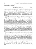
A plot of the first ITS [p
L,t
,p
U,t
] is presented in Figure 10.5.
Following the classical regression approach to ITS, we are interested in the
properties and time series regression models of the components of the inter-
val, i.e., p
L
,p
U
,p
C

, and p
R
. We present the most significant and unrestricted
time series models for [p
L,t
,p
U,t
] and p
C,t
,p
R,t
in the spirit of the regression
proposals of Billard and Diday (2000, 2002) and Lima Neto and de Carvalho
(2008) reviewed in the previous sections. To save space we omit the univari-
ate modeling of the components of the interval but these results are available
upon request. However, we need to report that for p
L
and p
U
, we cannot
reject a unit root, which is expected because these are price levels of the
SP500, and that p
C
has also a unit root because it is the sum of two unit root
processes. In addition, p
L
and p
U
are cointegrated of order one with coin-
tegrating vector (1, −1), which implies that p

R
is a stationary process given
Jan00 Jan01 Jan02 Jan03 Jan04 Jan05 Jan06
800
900
1000
1100
1200
1300
1400
1500
FIGURE 10.5
ITS of the weekly low/high from January 2000 to December 2006.

P1: GOPAL JOSHI
November 3, 2010 17:15 C7035 C7035˙C010
Forecasting with Interval and Histogram Data 263
that p
R
= (p
U
− p
L
)/2. Following standard model selection criteria and time
series specification tools, the best model for p
C,t
,p
R,t
 is a VAR(3) and for
[p

L,t
,p
U,t
] a VEC(3). The estimation results are presented in Tables A.1 and
A.2 in the appendix.
In Table A.1, the estimation results for p
C,t
,p
R,t
in both periods are very
similar. The radius p
R,t
exhibits high autoregressive dependence and it is
negatively correlated with the previous change in the center of the interval
p
C,t−1
so that positive surprises in the center tend to narrow down the inter-
val. On the other hand p
C,t
has little linear dependence and it is not affected
by the dynamics of the radius. There is Granger causality from the center
to the radius, but not vice versa. The radius equation enjoys a relative high
adjusted R-squared of about 40% while the center is basically not linearly
predictable. In general terms, there is a strong similarity between the model-
ing of p
C,t
,p
R,t
 and the most classical modeling of volatility with ARCH
models for financial returns. The processes p

R,t
and the conditional variance
of an asymmetric ARCH model, i.e., ␴
2
t |t−1
= ␣
0
+␣
1
ε
2
t−1
+␣
2
ε
t−1
+␤␴
2
t−1 |t−2
,
share the autoregressive nature and the well-documented negative correla-
tion of past innovations and volatility. The unresponsiveness of the center to
the information in the dynamics of the radius is also similar to the findings
in ARCH-in-mean processes where it is difficult to find significant effects of
volatility on the return process.
In Table A.2, we report the estimation results for [p
L,t
,p
U,t
] for both periods

2000–2005 and 2002–2007. In general, there is much less linear dependence in
the short-run dynamics of [p
L,t
,p
U,t
], which is expected as we are modeling
financial prices. There is Granger-causality running both ways, from p
L
to p
U
and vice versa. Overall, the 2002-2007 period seems to be noisier
(R-squared of 14%) than the 2000–2005 (R-squared of 20%–16%).
Based on the estimation results of the VAR(3) and VEC(3) models, we pro-
ceed toconstructtheone-step-ahead forecastoftheinterval[ˆp
L,t+1 |t
, ˆp
U,t+1 |t
].
Wealso implementtheexponential smoothingmethodsand thek-NNmethod
for ITS proposed in the above sections and compare their respective fore-
casts. For the smoothing procedure, the estimated value of ␣ is ˆ␣ = 0.04 in
the estimation period 2000–2005 and ˆ␣ = 0.03 in 2002–2007. We have im-
plemented the k-NN with equal weights and with inversely proportional
as in Equation 10.31. In the period 2000–2005, the numbers of neighbors is
ˆ
k = 23 (equal weights) and
ˆ
k = 24 (proportional weights); in 2002–2007
ˆ
k = 18 for the k-NN with equal weights and

ˆ
k = 24 for proportional weights.
In both estimation periods, the length of the vector is
ˆ
d = 2 for the k-NN
with equal weights and
ˆ
d = 3 for the proportional weights. The estima-
tion of ␣, k, and d has been performed by minimizing the mean distance
MDE (Equation 10.22) with q = 2. In both methods, smoothing and k-NN,
the centers of the intervals have been first-differenced to proceed with the
estimation and forecasting. However, in the following comparisons, the es-
timated differenced centers are transformed back to present the estimates
and forecasts in levels. In Table 10.1 we show the performance of the five
models measured by the MDE (q = 2) in the estimation and prediction

P1: GOPAL JOSHI
November 3, 2010 17:15 C7035 C7035˙C010
264 Handbook of Empirical Economics and Finance
TABLE 10.1
Performance of the Forecasting Methods: MDE (q = 2)
Period 2000–2006 Period 2002–2008
Estimation Prediction Estimation Prediction
Models 2000–2005 2006 2002–2007 2008
VAR(3) 9.359 6.611 7.614 15.744
VEC(3) 9.313 6.631 7.594 15.766
k-NN (eq.weights) 9.419 6.429 7.625 15.865
k-NN (prop.weights) 9.437 6.303 7.617 16.095
Smoothing 9.833 6.698 7.926 16.274
Naive 10.171 7.056 8.231 16.549

periods. We have also added a “naive” model that does not entail any es-
timation and whose forecast is the observation in the previous period, i.e.,
[ˆp
L,t+1 |t
, ˆp
U,t+1 |t
] = [p
L,t
,p
U,t
].
For both low- and high-volatility periods the performance ranking of the
six models is very similar. The worst performer is the naive model followed by
thesmoothingmodel.In 2006, the k-NNproceduresaresuperiorto the VAR(3)
and VEC(3) models, but in 2008 the VAR and VEC systems perform slightly
better than the k-NNs. The high-volatility year 2008 is clearly more difficult
to forecast, the MDE in 2008 is twice as much as the MDE in the estimation
period 2002–2007. On the contrary, in the low volatility year 2006, the MDE
in the prediction period is about 30% lower than the MDE in the estimation
period 2000–2005. A statistical comparison of the MDEs of the five models in
relation to the naive model is provided by the Diebold and Mariano test of
unconditional predictability(DieboldandMariano 1995). The null hypothesis
to test is the equality of the MDEs, i.e., H
0
: E(D
2
(naive)
−D
2
(other)

) = 0 versus H
1
:
E(D
2
(naive)
− D
2
(other)
) > 0. If the null hypothesis is rejected the other model is
superior to the naive model. The results of this test are presented in Table 10.2.
In 2006 all the five models are statistically superior to the benchmark naive
model. In 2008 the smoothing procedure and the k-NN with proportional
weights are statistically equivalent to the naive model while the remaining
three models outperform the naive.
TABLE 10.2
Results of the Diebold and Mariano Test
T-Test for
H
0
: E(D
2
(naive)
− D
2
(other)
)=0
Models 2006 2008
VAR(3) 2.86 2.67
VEC(3) 2.26 2.46

k-NN(eq.weights) 3.55 2.43
k-NN(prop.weights) 4.17 1.79
Smoothing 5.05 1.15

P1: GOPAL JOSHI
November 3, 2010 17:15 C7035 C7035˙C010
Forecasting with Interval and Histogram Data 265
We also perform a complementary assessment of the forecasting ability of
the five models by running some regressions of the Mincer–Zarnowitz type.
In the prediction periods, for the minimum p
L
and the maximum p
U
, we
run separate regressions of the realized observations on the predicted ob-
servations as in p
L,t
= c + ␤ ˆp
L,t
+ ε
t
and p
U,t
= c + ␤ ˆp
U,t
+ υ
t
. Under a
quadratic loss function, we should expect an unbiased forecast, i.e., ␤ = 1
and c = 0. However, the processes p

L,t
and ˆp
L,t
are I (1) and, as expected,
cointegrated, so that these regressions should be performed with care. The
point of interest is then to test for a cointegration vector of (1, −1). To test this
hypothesis using an OLS estimator with the standard asymptotic distribu-
tion, we need to consider that in the I(1) process ˆp
L,t
, i.e., ˆp
L,t
= ˆp
L,t−1
+ ␯
t
,
the innovations ε
t
and ␯
t
are not independent; in fact because ˆp
L,t
is a forecast
of p
L,t
the correlation ␳(␯
t+i
, ε
t
) = 0 for i > 0. To remove this correlation,

the cointegrating regression will be augmented with some terms to finally
estimate a regression as p
L,t
= c + ␤ ˆp
L,t
+

i
␥
i
 ˆp
L,t+i
+ e
t
(the same ar-
gument applies to p
U,t
). The hypothesis of interest is H
0
: ␤ = 1 versus
H
1
: ␤ = 1. A t-statistic for this hypothesis will be asymptotically standard
normal distributed. We may also need to correct the t-test if there is some
serial correlation in e
t
. In Table 10.3 we present the testing results.
We reject the null for the smoothing method for both prediction periods
and for both p
L,t

and p
U,t
processes. Overall the prediction is similar for 2006
and 2008. The VEC(3) and the k-NN methods deliver better forecasts across
the four instances considered. For those models in which we fail to reject
H
0
: ␤ = 1, we also calculate the unconditional average difference between
the realized and the predicted values, i.e, ¯p =

t
( p
t
− ˆp
t
)/T. The magnitude
of this average is in the single digits, so that for all purposes, it is insignificant
given that the level of the index is in the thousands. In Figure 10.6 we show
the k-NN (equal weights)-based forecast of the interval low/highof the SP500
index for November and December 2006.
TABLE 10.3
Results of the t-Test for Cointegrating Vector (1, −1)
Asymptotic (Corrected) t-Test
H
0
: ␤ = 1 versus H
1
: ␤ =1
p
t

= c + ␤ˆp
t
+

i
␥
i
Δˆp
t+i
+ e
t
2006 2008
min: p
L,t
max: p
U,t
min: p
L,t
max: p
U,t
VAR(3) 3.744
∗
−1.472 3.024
∗
−2.712
∗
VEC(3) 1.300 0.742 2.906
∗
−2.106
k-NN (eq.weights) 0.639 −4.191

∗
1.005 −2.270
k-NN (prop.weights) 3.151
∗
−2.726
∗
1.772 −1.731
Smoothing −3.542
∗
−2.544
∗
2.739
∗
−3.449
∗
∗
Rejection of the null hypothesis at the 1% significance level.

P1: GOPAL JOSHI
November 3, 2010 17:15 C7035 C7035˙C010
266 Handbook of Empirical Economics and Finance
Nov06 Dec06
1360
1370
1380
1390
1400
1410
1420
1430

FIGURE 10.6
k-NN based forecast (black) of the low/high prices of the SP500; realized ITS (grey).
10.3 Histogram Data
In this section, our premise is that the data is presented to the researcher as
a frequency distribution, which may be the result of an aggregation proce-
dure, or the description of a population or any other grouped collective. We
start by describing histogram data and some univariate descriptive statis-
tics. Our main objective is to present the prediction problem by defining a
histogram time series (HTS) and implementing smoothing techniques and
nonparametric methods like the k-NN algorithm. As we have seen in the sec-
tion on interval data, these two methods require the calculation of suitable
averages. To this end, instead of relying on the arithmetic of histograms, we
introduce the barycentric histogram that is an average of a set of histograms.
The choice of appropriate distance measures is key to the calculation of the
barycenter, and eventually of the forecast of a HTS.
10.3.1 Preliminaries
Given avariableofinterest X,wecollectinformationon a groupofindividuals
or units that belong to a set S. For every element i ∈ S, we observe a datum
such as
h
X
i
={([x]
i1
, ␲
i1
), , ([x]
in
i
, ␲

in
i
)}, for i ∈ S, (10.32)
where ␲
ij
, j = 1, ,n
i
is a frequency that satisfies ␲
ij
≥ 0 and

n
i
j=1
␲
ij
=
1; and [x]
ij
⊆ R, ∀i, j, is an interval (also known as bin) defined as [x]
ij
≡
[x
Lij
,x
Uij
) with −∞ < x
Lij
≤ x
Uij

< ∞ and x
Ui j−1
≤ x
Lij
∀i, j, for j ≥ 2. The
datum h
X
i
is a histogram and the data set will be a collection of histograms
{h
X
i
,i= 1, ,m}.

P1: GOPAL JOSHI
November 3, 2010 17:15 C7035 C7035˙C010
Forecasting with Interval and Histogram Data 267
As in the case of interval data, we could summarize the histogram data set
by its empirical density function from which the sample mean and the sample
variance can be calculated (Billard and Diday 2006). The sample mean is
¯
X =
1
2m
m

i=1
n
i


j=1
(x
Uij
+ x
Lij
)␲
ij
, (10.33)
which is the average of the weighted centers for each interval; and the sample
variance is
S
2
X
=
1
3m
m

i=1
n
i

j=1

x
2
Uij
+ x
Uij
x

Lij
+ x
2
Lij

␲
ij
−
1
4m
2

m

i=1
n
i

j=1
(x
Uij
+ x
Lij
)␲
ij

2
,
which combines the variability of the centers as well as the intra-interval
variability. Note that the main difference between these sample statistics and

those in Equations 10.7 and 10.9 for interval data is the weight provided by
the frequency ␲
i, j
associated with each interval [x]
i, j
.
Next, we proceed with the definition of a histogram random variable. Let
(, F,P) be a probability space, where  is the set of elementary events, F is
the ␴-field of events and P : F → [0, 1] the ␴-additive probability measure;
and define a partition of  into sets A
X
(x) such that A
X
(x) ={␻ ∈ |X(␻) =
x}, where x ∈{h
X
i
,i= 1, ,m}.
Definition 10.4 A mapping h
X
: F →{h
X
i
}, such that, for all x ∈{h
X
i
,i =
1 m} there is a set A
X
(x) ∈ F, is called a histogram random variable.

Then, the definition of stochastic process follows as:
Definition 10.5 A histogram-valued stochastic process is a collection of histogram
random variables that are indexed by time, i.e., {h
X
t
} for t ∈ T ⊂ R, with each h
X
t
following Definition 10.4.
A histogram-valued time series is a realization of a histogram-valued
stochastic process and it will be equivalently denoted as {h
X
t
}≡{h
X
t
,t=
1, 2, ,T}.
10.3.2 The Prediction Problem
In this section, we propose a dissimilarity measure for HTS based on a dis-
tance. We present two distance measures that will play a key role in the esti-
mation and prediction stages. They will also be instrumental to the definition
of a barycentric histogram, which will be used as the average of a set of
histograms. Finally, we will present the implementation of the prediction
methods.

P1: GOPAL JOSHI
November 3, 2010 17:15 C7035 C7035˙C010
268 Handbook of Empirical Economics and Finance
10.3.2.1 Accuracy of the Forecast

Suppose that we construct a forecast for {h
X
t
}, which we denote as {
ˆ
h
X
t
}. It is
sensible to define the forecast error as the difference h
X
t
−
ˆ
h
X
t
. However, the
difference operator based on histogram arithmetic (Colombo and Jaarsma
1980) does not provide information on how dissimilar the histograms h
X
t
and
ˆ
h
X
t
are. In order to avoid this problem, Arroyo and Mat´e (2009) pro-
pose the mean distance error (MDE), which in its most general form is de-
fined as

MDE
q
({h
X
t
}, {
ˆ
h
X
t
}) =


T
t=1
D
q
(h
X
t
,
ˆ
h
X
t
)
T

1
q

, (10.34)
where D(h
X
t
,
ˆ
h
X
t
) is adistancemeasuresuchastheWassersteinorthe Mallows
distance to be defined shortly and q is the order of the measure, such that for
q = 1 the resulting accuracy measure is similar to the MAE and for q = 2to
the RMSE.
Consider two density functions, f (x) and g
(
x
)
, with their correspond-
ing cumulative distribution functions (CDF), F (x) and G(x), the Wasserstein
distance between f (x) and g
(
x
)
is defined as
D
W
( f, g) =

1
0

|F
−1
(t) − G
−1
(t)|dt, (10.35)
and the Mallows as
D
M
( f, g) =


1
0
(F
−1
(t) − G
−1
(t))
2
dt, (10.36)
where F
−1
(t) and G
−1
(t) with t ∈ [0, 1] are the inverse CDFs of f (x) and g(x),
respectively. The dissimilarity between two functions is essentially measured
by how far apart their t-quantiles are, i.e., F
−1
(t) − G
−1

(t). In the case of
Wasserstein, the distance is defined in the L
1
norm and in the Mallows in
the L
2
norm. When considering Equation 10.34, D(h
X
t
,
ˆ
h
X
t
) will be calculated
by implementing the Wasserstein or Mallows distance. By using the defini-
tion of the CDF of a histogram in Billard and Diday (2006), the Wasserstein
and Mallows distances between two histograms h
X
and h
Y
can be written
analytically as functions of the centers and radii of the histogram bins, i.e.,
D
W
(h
X
,h
Y
) =

n

j=1
␲
j
|x
Cj
− y
Cj
| (10.37)
D
2
M
(h
X
,h
Y
) =
n

j=1
␲
j

(x
Cj
− y
Cj
)
2

+
1
3
(x
Rj
− y
Rj
)
2

. (10.38)

P1: GOPAL JOSHI
November 3, 2010 17:15 C7035 C7035˙C010
Forecasting with Interval and Histogram Data 269
10.3.2.2 The Barycentric Histogram
Given a set of K histograms h
X
k
with k = 1, ,K, the barycentric histogram
h
X
B
is the histogram that minimizes the distances between itself and all the
K histograms in the set. The optimization problem is
min
h
X
B
K


k=1

D
r
(h
X
k
,h
X
B
)

1/r
, (10.39)
where D(h
X
k
,h
X
B
) is a distance measure. The concept is introduced by Ir-
pino and Verde (2006) to define the prototype of a cluster of histogram data.
As Verde and Irpino (2007) show, the choice of the distance determine the
properties of the barycenter.
When the chosen distance is Mallows, for r = 2, the optimal barycentric
histogram h
∗
X
B

has the following center/radius characteristics. Once the k
histograms are rewritten in terms of n
∗
bins, for each bin j = 1, ,n
∗
, the
barycentric center x
∗
Cj
is the mean of the centers of the corresponding bin in
each histogram and the barycentric radius x
∗
Rj
is the mean of the radii of the
corresponding bin in each of the K histograms,
x
∗
Cj
=

K
k=1
x
Ckj
K
(10.40)
x
∗
Rj
=


K
k=1
x
Rkj
K
. (10.41)
When the distance is Wasserstein, for r = 1 and for each bin j = 1, ,n
∗
,
the barycentric center x
∗
Cj
is the median of the centers of the corresponding
bin in each of the K histograms,
x
∗
Cj
= median(x
Ckj
) for k = 1, ,K (10.42)
and the radius x
∗
Rj
is the corresponding radius of thebin wherethe median x
∗
Cj
falls among the K histograms. For more details on the optimization problem,
please see Arroyo and Mat´e (2009).
10.3.2.3 Exponential Smoothing

The exponential smoothing method can be adapted to histogram time series
by replacing averages with the barycentric histogram, as it was shown in
Arroyo and Mat´e (2008).
Let{h
X
t
}t = 1, ,Tbeahistogramtimeseries,theexponentiallysmoothed
forecast is given by the following equation
ˆ
h
X
t+1
= ␣h
X
t
+ (1 −␣)
ˆ
h
X
t
, (10.43)
where ␣ ∈ [0, 1]. Since the right-hand side is a weighted average of his-
tograms,wecanuse thebarycenterapproach so thattheforecastisthesolution

P1: GOPAL JOSHI
November 3, 2010 17:15 C7035 C7035˙C010
270 Handbook of Empirical Economics and Finance
to the following optimization exercise
ˆ
h

X
t+1
≡ arg min
ˆ
h
X
t+1

␣D
2
(
ˆ
h
X
t+1
,h
X
t
) + (1 −␣)D
2
(
ˆ
h
X
t+1
,
ˆ
h
X
t

)

1/2
, (10.44)
where D(·, ·) is the Mallows distance. The use of the Wasserstein distance is
not suitable in this case because of the properties of the median, which will
ignore the weighting scheme (with the exception of ␣ = 0.5) so intrinsically
essential to the smoothing technique. For further developments of this issue
see Arroyo, Gonz´alez-Rivera, Mat´e and Mu˜noz-San Roque (2010).
For t large, the recursive form (Equation 10.43) can be easily rewritten as a
moving average
ˆ
h
X
t+1

t

j=1
␣(1 − ␣)
j−1
h
X
t−( j−1)
, (10.45)
which in turn can also be expressed as the following optimizations problem
ˆ
h
X
t+1

≡ arg min
ˆ
h
X
t+1

t

j=1
␣(1 − ␣)
j−1
D
2
(
ˆ
h
X
t+1
,h
X
t−( j−1)
)

1/2
, (10.46)
with D(·, ·) as the Mallows distance. The Equations 10.44 and 10.46 are equiv-
alent.
Figure 10.7 shows an example of the exponential smoothing using Equa-
tion10.44for thehistogramsh
X

t
={([19, 20), 0.1), ([20, 21), 0.2), ([21, 22], 0.7)}
and
ˆ
h
X
t
={([0, 3), 0.35), ([3, 6), 0.3), ([6, 9], 0.35)} with ␣ = 0.9 and ␣ = 0.1.
In both cases, the resulting histogram averages the location, the support, and
the shape of both histograms h
X
t
and
ˆ
h
X
t
in a suitable way.
0.8
1
0.6
0.4
0.2
0
0 5 10 15 20
0.8
1
0.6
0.4
0.2

0
0 5 10 15 20
FIGURE 10.7
Exponential smoothing of histograms using the recursive formulation with ␣ = 0.9 (left) and
␣ = 0.1 (right). In each part of the figure, the barycenter is the dash-lined histogram.

P1: GOPAL JOSHI
November 3, 2010 17:15 C7035 C7035˙C010
Forecasting with Interval and Histogram Data 271
10.3.2.4 k-NN Method
The adaptation of the k-NN method to forecast HTS was proposed by Arroyo
and Mat´e (2009). The method consists of similar steps to those described in
the interval section:
1. The HTS,{h
X
t
}witht = 1, ,T,isorganizedasa seriesofd-dimensional
histogram-valued vectors {h
d
X
t
} where
h
d
X
t
= (h
X
t
,h

X
t−1
, ,h
X
t−(d−1)
)

, (10.47)
where d ∈ N is the number of lags and t = d, ,T.
2. Wecomputethe dissimilaritybetweenthemostrecenthistogram-valued
vector h
d
X
T
= (h
X
T
,h
X
T−1
, ,h
X
T−(d−1)
)

and the rest of the vectors in {h
d
X
t
}

by implementing the following distance measure
D
t
(h
d
X
T
,h
d
X
t
) =


d
i=1

D
q
(h
X
T−i+1
,h
X
t−i+1
)

d

1

q
, (10.48)
where D
q
(h
X
T−i+1
,h
X
t−i+1
) is the Mallows or the Wasserstein distance of
order q.
3. Once the dissimilarity measures are computed for each h
d
X
t
,t= T −
1,T−2, ,d, we select the k closest vectors to h
d
X
T
. These are denoted
by h
d
X
T
1
,h
d
X

T
2
, ,h
d
X
T
k
.
4. Given the k closest vectors, their subsequent values, h
X
T
1
+1
,h
X
T
2
+1
, ,
h
X
T
k
+1
, are averaged by means of the barycenter approach to obtain the
final forecast
ˆ
h
X
T+1

as in
ˆ
h
X
T+1
≡ arg min
ˆ
h
X
T+1

k

p=1
␻
p
D
r
(
ˆ
h
X
T+1
,h
X
T
p
+1
)


1/r
, (10.49)
where D(
ˆ
h
X
T+1
,h
X
T
p
+1
) is the Mallows distance with r = 2 or the Wasser-
stein distance with r = 1, h
X
T
p
+1
is the consecutive histogram in the
sequence h
d
X
T
p
, and ␻
p
is the weight assigned to the neighbor p, with
␻
p
≥ 0 and


k
p=1
␻
p
= 1. As in the case of the interval-valued data, the
weights may be assumed to be equal for all the neighbors ␻
p
= 1/k ∀p,
or inversely proportional to the distance between the last sequence h
d
X
T
and the considered sequence h
d
X
T
p
.
The optimal values,
ˆ
k and
ˆ
d, which minimize the mean distance error
(Equation 10.34) in the estimation period, are obtained by conducting a two-
dimensional grid search.

P1: GOPAL JOSHI
November 3, 2010 17:15 C7035 C7035˙C010
272 Handbook of Empirical Economics and Finance

10.3.3 Histogram Forecast for SP500 Returns
In this section, we implement the exponential smoothing and the k-NN meth-
ods to forecast the one-step-ahead histogram of the returns to the constituents
of the SP500 index. We collect the weekly returns of the 500 firms in the index
from 2002 to 2005. We divide the sample into an estimation period of 156
weeks running from January 2002 to December 2004, and a prediction period
of 52 weeks that goes from January 2005 to December 2005. The histogram
data set consists of 208 weekly equiprobable histograms. Each histogram has
four bins, each one containing 25% of the firms’ returns.
For the smoothing procedure, the estimated value of ␣ is ˆ␣ = 0.13. We have
implemented the k-NN with equal weights and with inversely proportional
as in Equation 10.31 using the Mallows and Wasserstein distances. With the
Mallows distance, the estimated numbers of neighbors is
ˆ
k = 11 and the
length of the vector is
ˆ
d = 9 for both weighting schemes. With the Wasserstein
distance,
ˆ
k = 12,
ˆ
d = 9 (equal weights), and
ˆ
k = 17,
ˆ
d = 8 (proportional
weights). The estimation of ␣, k, and d has been performed by minimizing
the Mallows MDE with q = 1, except for the Wasserstein-based k-NN which
used theWassersteinMDE with q = 1. In Table10.4,weshowthe performance

of the five models measured by the Mallows-based MDE (q = 1) in the
estimation and prediction periods. We have also added a “naive” model that
does not entail any estimation and for which the one-step-ahead forecast is
the observation in the previous period, i.e.,
ˆ
h
X
t+1 |t
= h
X
t
.
In the estimation and prediction period, the naive model is clearly out-
performed by the rest of the five models. In the estimation period, the five
models exhibit similar performance with a MDE of 4.9 approximately. In the
prediction period, the exponential smoothing and the Wasserstein-based k-
NN seem to be superior to the Mallows-based k-NN. We should note that
the MDEs in the prediction period are about 11% lower than the MDEs in the
estimation period.
For the prediction year 2005, we provide a statistical comparison of the
MDEs of the five models in relation to the naive model by implementing
the Diebold and Mariano test of unconditional predictability (Diebold and
Mariano 1995). The null hypothesis to test is the equality of the MDEs, i.e.,
H
0
: E(D
(naive)
− D
(other)
) = 0 versus H

1
: E(D
(naive)
− D
(other)
) > 0. If the null
TABLE 10.4
Performance of the Forecasting Methods: MDE
(q = 1)
Estimation Prediction
Models 2002–2004 2005
Mall. k-NN (eq.weights) 4.988 4.481
Mall. k-NN (
prop.weights) 4.981 4.475
Wass. k-NN (
eq.weights) 4.888 4.33
Wass. k-NN (
prop.weights) 4.882 4.269
Exp. Smoothing 4.976 4.344
Naive 6.567 5.609

P1: GOPAL JOSHI
November 3, 2010 17:15 C7035 C7035˙C010
Forecasting with Interval and Histogram Data 273
TABLE 10.5
Results of the Diebold and Mariano Test
t-Test for
H
0
: E(D

(naive)
− D
(other)
)=0
Models 2005 Prediction Year
Mall. k-NN(eq.weights) 2.32
Mall. k-NN
(prop.weights)
2.69
Wass. k-NN
(eq.weights) 2.29
Wass. k-NN
(prop.weights)
2.29
Exp. smoothing 3.08
hypothesis is rejected, the “other” model is superior to the naive model. The
results of this test are presented in Table 10.5.
In 2005, all the five models are statistically superior to the benchmark naive
model, though the rejection of the null is stronger for the exponential smooth-
ing and the Mallows-based k-NN models with proportional weights.
In Figure 10.8, we present the 2005 one-step-ahead histogram forecast ob-
tained with the exponential smoothing procedure and we compare it to the
realized value. For each time period, we draw two histograms: the realized
histogram (the right one) and the forecast histogram (the left one). Overall the
forecast follows very closely the realized value except for those observations
that have extreme returns. The fit can be further appreciated when we zoom
in the central 50% mass of the histograms (Figure 10.9).
3-Jan 7-Feb 7-Mar 4-Apr 2-May 6-Jun 5-Jul 1-Aug 6-Sep 3-Oct 7-Nov 5-Dec
–80
–60

–40
–20
0
20
40
60
FIGURE 10.8
2005 realized histograms (the right ones) and exponential smoothed one-step-ahead histogram
forecasts (the left ones) for the HTS of SP500 returns. Weekly data.

P1: GOPAL JOSHI
November 3, 2010 17:15 C7035 C7035˙C010
274 Handbook of Empirical Economics and Finance
6-Sep 3-Oct 7-Nov 5-Dec
–8
–6
–4
–2
0
2
4
6
8
FIGURE 10.9
Zoom of Figure 10.8 from September to December 2005.
10.4 Summary and Conclusions
Large databases prompt the need for new methods of processing informa-
tion. In this article we have introduced the analysis of interval-valued and
histogram-valued data sets as an alternative to classical single-valued data
sets and we have shown the promise of this approach to deal with economic

and financial data.
With interval data, most of the current efforts have been directed to the
adaptation of classical regression models as the interval is decomposed into
two single-valued variables, either the center/radius or the min/max. The ad-
vantage of this decomposition is that classical inferential methods are avail-
able. Methodologies that analyze the interval per se fall into the realm of
random sets theory and though there is some important research on regres-
sion analysis with random sets, inferential procedures are almost nonexis-
tent. Being our current focus is the prediction problem, we have explored two
different venues to produce a forecast with interval time series (ITS). First,
we have implemented the classical regression approach to the analysis of
ITS, and secondly we have proposed the adaptation to ITS of filtering tech-
niques, such as smoothing, and nonparametric methods, such as the k-NN,
to ITS. The latter venue requires the use of interval arithmetic to construct
the appropriate averages and the introduction of distance measures to as-
sess the dissimilarity between intervals and to quantify the prediction error.
We have implemented these ideas with the SP500 index. We modeled the

P1: GOPAL JOSHI
November 3, 2010 17:15 C7035 C7035˙C010
Forecasting with Interval and Histogram Data 275
center/radius time series and the low/high time series of what we called
interval-valued dispersion of the SP500 index and compared their one-step-
ahead forecasts to those of asmoothing procedure and k-NN methods.A VEC
modelforthe low/highseriesandthek-NNmethodshave thebestforecasting
performance.
With histogram data, the analysis becomes more complex. Regression anal-
ysis with histograms is in its infancy and the venues for further develop-
ments are large. We have focused exclusively in the prediction problem with
smoothing methods and nonparametric methods. A key concept for the im-

plementation of these two procedures is the introduction of the barycentric
histogram that is a device that works as an average (weighted or unweighted)
of a set of histograms. As with ITS, the introduction of the appropriate dis-
tances to judge dissimilarities among histograms and to assess forecast errors
are fundamental ingredients in the analysis. The collection over time of cross-
sectionalreturns ofthefirms in theSP500index providesanice histogram time
series (HTS), on which we have implemented the aforementioned methods to
eventually producetheone-step-aheadhistogramforecast.Simplesmoothing
techniques seem to work remarkably well.
There are still many unexplored areas in ITS and HTS. A very important
question is the search for a model. This will require the understanding of the
notion of dependence in ITS and HTS. A first step in this direction is pro-
vided by Gonz´alez-Rivera and Arroyo (2010) who construct autocorrelation
functions for HTS and ITS. From an econometric point of view, model build-
ing requires further research on identification, estimation, testing, and model
selection procedures. Economic and financial questions will benefit greatly
from this new approach to the analysis of large data sets.
10.5 Acknowledgment
We thank the referees and the editors for useful and constructive comments.
Arroyoacknowledgessupport fromtheSpanishCouncil for Science andInno-
vation (grant TIN2008-06464-C03-01) and from the ProgramadeCreaci
´
on y Con-
solidaci
´
ondeGrupos deInvestigaci
´
onUCM-BancoSantander. Gonz´alez-Rivera ac-
knowledges the financial support provided by the University Scholar Award.
Mat´e acknowledges the financial support provided by the project “Fore-

casting models from symbolic data (PRESIM)” from Universidad Pontificia
Comillas.
Appendix
Estimation Results for ITS SP500 Index

P1: GOPAL JOSHI
November 3, 2010 17:15 C7035 C7035˙C010
276 Handbook of Empirical Economics and Finance
TABLE A.1
Estimation of the VAR(3) Model for the Differenced Center and Radius
Time Series
Estimation Sample 2000–2005 Estimation Sample 2002–2007
VAR D(Cen) Rad VAR D(Cen) Rad
D(Cen(−1)) 0.33218 −0.09764 D(Cen(−1)) 0.279225 −0.074092
0.0262 0.00997 0.02619 0.00978
[ 12.6803] [−9.79410] [10.6611] [−7.57934]
D(Cen(−2)) −0.181348 −0.001809 D(Cen(−2)) −0.092471 −0.010534
0.02742 0.01043 0.02713 0.01012
[−6.61378] [−0.17332] [−3.40879] [−1.04037]
D(Cen(−3)) 0.050564 0.00429 D(Cen(−3)) 0.006178 −0.013364
0.02616 0.00996 0.02629 0.00981
[ 1.93281] [ 0.43091] [ 0.23500] [−1.36214]
Rad(−1) 0.066659 0.150616 Rad(−1) −0.00284 0.152907
0.06593 0.02509 0.06731 0.02512
[ 1.01103] [ 6.00287] [−0.04219] [ 6.08652]
Rad(-2) −0.049629 0.313259 Rad(-2) 0.046537 0.27345
0.06319 0.02405 0.0649 0.02422
[−0.78541] [ 13.0270] [0.71705] [11.2886]
Rad(-3) 0.129442 0.285272 Rad(-3) −0.01386 0.276629
0.0648 0.02466 0.06635 0.02477

[1.99747] [11.5678] [−0.20888] [11.1699]
C −1.319847 2.088036 C −0.045805 2.074405
0.60607 0.23064 0.5355 0.19987
[−2.17772] [9.05315] [−0.08554] [10.3788]
TABLE A.2
Estimation of the VEC(3) Model for Low/High Time Series
Estimation Sample 2000–2005 Estimation Sample 2002–2007
Error Correction: D(Low) D(High) Error Correction: D(Low) D(High)
CointEq1 −0.438646 0.007023 CointEq1 −0.124897 0.121926
0.05364 0.04758 0.04103 0.03692
[−8.17770] [0.14761] [−3.04419] [3.30283]
D(Low(-1)) 0.112549 0.515586 D(Low(-1)) −0.165406 0.425054
0.05429 0.04816 0.0489 0.044
[2.07293] [10.7050] [−3.38238] [9.66024]
D(Low(-2)) −0.093605 0.193326 D(Low(-2)) −0.314249 0.130253
0.0505 0.0448 0.04863 0.04375
[−1.85344] [4.31532] [−6.46233] [2.97698]
D(Low(-3)) 0.026446 0.112943 D(Low(-3)) −0.15041 0.061275
0.0396 0.03512 0.0399 0.0359
[0.66790] [3.21547] [−3.76992] [1.70691]

P1: GOPAL JOSHI
November 3, 2010 17:15 C7035 C7035˙C010
Forecasting with Interval and Histogram Data 277
TABLE A.2 (Continued)
Estimation of the VEC(3) Model for Low/High Time Series
Estimation Sample 2000–2005 Estimation Sample 2002–2007
Error Correction: D(Low) D(High) Error Correction: D(Low) D(High)
D(High(-1)) 0.313542 −0.287591 D(High(-1)) 0.524179 −0.221533
0.05905 0.05238 0.05188 0.04668

[5.30959] [−5.49018] [10.1046] [−4.74625]
D(High(-2)) −0.073453 −0.382411 D(High(-2)) 0.248088 −0.239401
0.05604 0.04971 0.05323 0.04789
[−1.31078] [−7.69307] [4.66085] [−4.99871]
D(High(-3)) 0.04646 −0.065429 D(High(-3)) 0.182654 −0.073329
0.04356 0.03864 0.04262 0.03835
[1.06663] [−1.69337] [4.28593] [−1.91234]
C −0.064365 −0.118124 Cointegrating Eq: CointEq1
0.28906 0.25642 Low(-1) 1
[−0.22267] [−0.46068] High(-1) −1.002284
Cointegrating Eq: Co-intEq1 0.00318
Low(-1) 1[−315.618]
High(-1) −1.001255 C 16.82467
0.00268 3.81466
[−373.870] [ 4.41053]
@TREND(1) −0.012818
0.00105
[−12.1737]
C 27.97538
References
Alizadeh, S., M. Brandt, and F. Diebold. 2002. Range-based estimation of stochastic
volatility models. Journal of Finance 57(3):1047–1091.
Arroyo, J., R. Esp´ınola, and C. Mat´e. 2010. Different approaches to forecast interval
time series: a comparison in finance. Computational Economics Forthcoming.
Arroyo, J., G. Gonz´alez–Rivera, C. Mat´e, and A. Mu˜noz–San Roque. 2010. Smooth-
ing methods for histogram-valued time series. An application to value-at-risk.
Working paper, Department of Computer Science and Artificial Intelligence, Uni-
versidad Complutense de Madrid, Madrid. Spain.
Arroyo, J., and C. Mat´e. 2006. Introducing interval time series: accuracy measures.
In COMPSTAT 2006, Proceedings in Computational Statistics. Heidelberg: Physica-

Verlag, pp. 1139–1146.
Arroyo, J., and C. Mat´e. 2008. Forecasting time series of observed distributions with
smoothing methods based on the barycentric histogram. In Computational Intelli-
gence in Decision and Control. Proceedings of the 8th International FLINS Conference,
pp. 61–66. Singapore: World Scientific.
Arroyo, J., and C. Mat´e. 2009. Forecasting histogram time series with k-nearest neigh-
bours methods. International Journal of Forecasting 25(1):192–207.

P1: GOPAL JOSHI
November 3, 2010 17:15 C7035 C7035˙C010
278 Handbook of Empirical Economics and Finance
Ball, C., and W. Torous. 1984. The maximim likelihood estimation of security price
volatility: theory, evidence, and an application to option pricing. Journal of Busi-
ness 57(1):97–112.
Bertrand, P., and F. Goupil. 2000. Descriptive statistics for symbolic data, Analysis of
SymbolicData. ExploratoryMethodsforExtractingStatistical InformationfromComplex
Data. Berlin: Springer. pp. 103–124.
Billard, L., and E. Diday. 2000. Regression analysis for interval-valued data. In Data
Analysis, Classification and Related Methods: Proceedings of the 7th Conference of the
IFCS, IFCS 2002. Berlin: Springer. pp. 369–374.
Billard,L.,and E. Diday.2002. Symbolic regressionanalysis. In Classification, Clustering
and Data Analysis: Proceedings of the 8th Conference of the IFCS, IFCS 2002. Berlin:
Springer. pp. 281–288.
Billard, L., and E. Diday. 2003. From the statistics of data to the statistics of knowledge:
symbolic data analysis. Journal of the American Statistical Association 98(462):470–
487.
Billard, L., and E. Diday. 2006. Symbolic Data Analysis: Conceptual Statistics and Data
Mining. 1st ed. Chichester: Wiley & Sons.
Blanco,
´

A., A. Colubi, N. Corral, and G. Gonz´alez-Rodr´ıguez. 2008. On a linear in-
dependence test for interval-valued random sets. In Soft Methods for Handling
Variability and Imprecision. Advances in Soft Computing. Berlin: Springer. pp. 111–
117.
Brito, P. 2007. Modelling and analysing interval data. In Proceedings of the 30th Annual
Conference of GfKl. Berlin: Springer. pp. 197–208.
Cheung, Y L., Y W. Cheung, and A. T. K. Wan. 2009. A high-low model of daily stock
price ranges. Journal of Forecasting 28(2):103–119.
Colombo, A., and R. Jaarsma. 1980. A powerful numericalmethodtocombine random
variables. IEEE Transactions on Reliability 29(2):126–129.
Diebold, F. X., and R. S. Mariano. 1995. Comparing predictive accuracy. Journal of
Business and Economic Statistics 13(3):253–263.
Garc´ıa-Ascanio, C., and C. Mat´e. 2010. Electric power demand forecasting us-
ing interval time series: a comparison between VAR and iMLP. Energy Policy
38(2):715–725.
Gardner, E. S. 2006. Exponential smoothing: the state of the art. Part 2. International
Journal of Forecasting 22(4): 637–666.
Garman, M. B., and M. J. Klass. 1980. On the estimation of security price volatilities
from historical data. Journal of Business 53(1):67–78.
Gonz´alez, L., F. Velasco, C. Angulo, J. A. Ortega, and F. Ruiz. 2004. Sobren´ucleos, dis-
tancias y similitudes entre intervalos. Inteligencia Artificial, Revista Iberoamericana
de IA 8(23):111–117.
Gonz´alez-Rivera, G., and J. Arroyo. 2010. Time series modeling of histogram-valued
data. The daily histogram time series of SP500 intradaily returns. International
Journal of Forecasting. Forthcoming.
Gonz´alez-Rivera, G., T H. Lee, and S. Mishra. 2008. Jumps in cross-sectional rank and
expected returns: a mixture model. Journal of Applied Econometrics 23:585–606.
Gonz´alez-Rodr´ıguez, G., A. Blanco, N. Corral, and A. Colubi. 2007. Least squares
estimation of linear regression models for convex compact random sets. Advances
in Data Analysis and Classification 1:67–81.

Han, A., Y. Hong, K. Lai, and S. Wang. 2008. Interval time series analysis with an
application to the sterling-dollar exchange rate. Journal of Systems Science and
Complexity 21(4):550–565.

P1: GOPAL JOSHI
November 3, 2010 17:15 C7035 C7035˙C010
Forecasting with Interval and Histogram Data 279
Irpino, A., and R. Verde. 2006. A new Wasserstein based distance for the hierarchical
clusteringof histogramsymbolic data. InData Scienceand Classification,Proceedings
of the IFCS 2006. Berlin: Springer. pp. 185–192.
Kulpa, Z. 2006. A diagrammatic approach to investigate interval relations. Journal of
Visual Languages and Computing 17(5):466–502.
Lima Neto, E. A., and F. d. A. T. de Carvalho. 2008. Centre and range method for fitting
a linear regression model to symbolic interval data. Computational Statistics and
Data Analysis 52:1500–1515.
Lima Neto, E. d. A., and F. d. A. T. de Carvalho. 2010. Constrained linear regression
models for symbolic interval-valued variables. Computational Statistics & Data
Analysis 54(2):333–347.
Maia, A. L. S., F. d. A. de Carvalho, and T. B. Ludermir. 2008. Forecasting models for
interval-valued time series. Neurocomputing 71(16–18):3344–3352.
Manski, C., and E. Tamer. 2002. Inference on regressions with interval data on a
regressor or outcome. Econometrica 70(2):519–546.
Moore, R. E. 1966. Interval Analysis. Englewood Cliffs, NJ: Prentice Hall.
Moore, R.E.,R.B. Kearfott, and M. J. Cloud (eds.) 2009. Introduction to Interval Analysis.
Philadelphia, PA: SIAM Press.
Parkinson, M. 1980. The extreme value method for estimating the variance of the rate
of return. The Journal of Business 53(1):61.
Rogers, L.,and S. Satchell.1991. Estimationvariancefromhigh,low, andclosing prices.
Annals of Applied Probability 1(4):504–512.
Verde, R., and A. Irpino. 2007. Dynamic clustering of histogram data: using the right

metric. In Selected Contributions in Data Analysis and Classification. Berlin: Springer.
pp. 123–134.
Yakowitz, S. 1987. Nearest-neighbour methods for time series analysis. Journal of Time
Series Analysis 8(2):235–247.
Yang, D., and Q. Zhang. 2000. Drift independent volatility estimation based on high,
low, open, and close prices. Journal of Business 73(3):477–492.
Zellner, A., and J. Tobias. 2000. A note on aggregation, disaggregation and forecasting
performance. Journal of Forecasting 19:457–469.

P1: GOPAL JOSHI
November 3, 2010 17:15 C7035 C7035˙C010

P1: BINAYA KUMAR DASH
November 1, 2010 14:37 C7035 C7035˙C011
11
Predictability of Asset Returns and the
Efficient Market Hypothesis
M. Hashem Pesaran
CONTENTS
11.1 Introduction 282
11.2 Prices and Returns 283
11.2.1 Single Period Returns 283
11.2.2 Multi-Period Returns 284
11.2.3 Overlapping Returns 284
11.3 Statistical Models of Returns 284
11.3.1 Percentiles, Critical Values, and Value at Risk 286
11.3.2 Measures of Departure from Normality 287
11.4 Empirical Evidence: Statistical Properties of Returns 287
11.4.1 Other Stylized Facts about Asset Returns 290
11.4.2 Monthly Stock Market Returns 291

11.5 Stock Return Regressions 293
11.6 Market Efficiency and Stock Market Predictability 294
11.6.1 Risk Neutral Investors 294
11.6.2 Risk Averse Investors 298
11.7 Return Predictability and Alternative Versions of the Efficient
Market Hypothesis 300
11.7.1 Dynamic Stochastic Equilibrium Formulations
and the Joint Hypothesis Problem 300
11.7.2 Information and Processing Costs and the EMH 301
11.8 Theoretical Foundations of the EMH 302
11.9 Exploiting Profitable Opportunities in Practice 307
11.10 New Research Directions 308
11.11 Acknowledgment 309
References 309
281

P1: BINAYA KUMAR DASH
November 1, 2010 14:37 C7035 C7035˙C011
282 Handbook of Empirical Economics and Finance
11.1 Introduction
Economists have long been fascinated by the nature and sources of variations
in the stock market. By the early 1970s a consensus had emerged among
financial economists suggesting that stock prices could be well approximated
by a random walk model and that changes in stock returns were basically
unpredictable. Fama (1970) provides an early, definitive statement of this
position. Historically, the “random walk” theory of stock prices was preceded
by theories relating movements in the financial markets to the business cycle.
A prominent example is the interest shown by Keynes in the variation instock
returns over the business cycle.
The efficient market hypothesis (EMH) evolved in the 1960s from the ran-

dom walk theory of asset prices advanced by Samuelson (1965). Samuelson
showed that in an informationally efficient market price changes must be un-
forecastable. Kendall (1953), Cowles (1960), Osborne (1959), Osborne (1962),
and many others had already provided statistical evidence on the random
nature of equity price changes. Samuelson’s contribution was, however, in-
strumental in providing academic respectability for the hypothesis, despite
the fact that the random walk model had been around for many years; having
been originally discovered by Louis Bachelier, a French statistician, back in
1900.
Although a number of studies found some statistical evidence against the
random walk hypothesis, these were dismissed as economically unimportant
(could not generate profitable trading rules in the presence of transaction
costs) and statistically suspect (could be due to data mining). For example,
Fama(1965),concludedthat “. . . thereisno evidence ofimportantdependence
from either an investment or a statistical point of view.” Despite its apparent
empirical success, the random walk model was still a statistical statement and
not a coherent theory of asset prices. For example, it need not hold in markets
populated by risk averse traders, even under market efficiency.
There now exist many different versions of the EMH, and one of the aims
of this chapter is to provide a simple framework where alternative versions of
the EMH can be articulated and discussed. We begin with an overview of the
statistical properties of asset returns at different frequencies (daily, weekly,
and monthly), and consider the evidence on return predictability, risk aver-
sion, and market efficiency. We then focus on the theoretical foundation of
the EMH, and show that market efficiency could coexist with heterogeneous
beliefs and individual “irrationality,” so long as individual errors are cross
sectionally weakly dependent in the sense defined by Chudik, Pesaran, and
Tosetti (2010). But at times of market euphoria or gloom these individual
errors are likely to become cross sectionally strongly dependent and the col-
lective outcome could display significant departures from market efficiency.

Market efficiency could be the norm, but most likely it will be punctuated by
episodes of bubbles and crashes. To test for such episodes we argue in favour
of compiling survey data on individual expectations of price changes that

P1: BINAYA KUMAR DASH
November 1, 2010 14:37 C7035 C7035˙C011
Predictability of Asset Returns and the Efficient Market Hypothesis 283
are combined with information on whether such expectations are compati-
ble with market equilibrium. A trader who believes that asset prices are too
high (low) might still expect further price rises (falls). Periods of bubbles and
crashes could result if there are sufficiently large numbers of such traders that
are prepared to act on the basis of their beliefs. The chapter also considers if
periods of market inefficiency can be exploited for profit. We conclude with
some general statements on new research directions.
We begin with some basic concepts and set out how returns are computed
over different horizons and assets, and discuss some of the known stylized
facts about returns by means of simple statistical models.
11.2 Prices and Returns
11.2.1 Single Period Returns
Let P
t
be the price of a security at date t. The absolute price change over the
period t − 1tot is given by P
t
− P
t−1
, the relative price change by
R
t
= (P

t
− P
t−1
)/P
t−1
the gross return (excluding dividends) on security by
1 + R
t
= P
t
/P
t−1
and the log price change by
r
t
=  ln(P
t
) = ln(1 + R
t
)
It is easily seen that for small relative price changes the log-price change and the
relative price change are almost identical.
In the case of daily observations when dividends are negligible, 100 · R
t
measures the percent return on the security, and 100 · r
t
is the continuously
compounded return. R
t
is also known as discretely compounded return. The

continuously compounded return, r
t
, is particularly convenient in the case
of temporal aggregation (multi-period returns; see Subsection 11.2.2), while
the discretely compounded returns are convenient for use in cross-sectional
aggregation, namely, aggregation of returns across different instruments in
a portfolio. For example, for a portfolio composed of N instruments with
weights w
i,t−1
,(

N
i=1
w
i,t−1
= 1,w
i,t−1
≥ 0) we have
R
pt
=
N

i=1
w
i,t−1
R
it
, (percent return)
r

pt
= ln

N

i=1
w
i.t−1
e
r
it

, (continuously compounded)
Often r
pt
is approximated by

N
i=1
w
i,t−1
r
it
.

P1: BINAYA KUMAR DASH
November 1, 2010 14:37 C7035 C7035˙C011
284 Handbook of Empirical Economics and Finance
When dividends are paid out we have
R

t
= (P
t
− P
t−1
)/P
t−1
+ D
t
/P
t−1
≈  ln(P
t
) + D
t
/P
t−1
where D
t
is the dividend paid out during the holding period.
11.2.2 Multi-Period Returns
Single-period price changes (returns) can be used to compute multi-period
price changes or returns. Denote the return over the most recent h periods by
R
t
(h) then (abstracting from dividends)
R
t
(h) =
P

t
− P
t−h
P
t−h
or
1 + R
t
(h) = P
t
/P
t−h
and
r
t
(h) = ln(P
t
/P
t−h
) = r
t
+r
t−1
+···+r
t−h+1
where r
t−i
, i = 0, 1, 2, ,h− 1 are the single-period returns. For example,
weekly returns are defined by r
t

(5) = r
t
+r
t−1
+···+r
t−4
. Similarly, since there
are 25 business days in one month, then the 1-month return can be computed
as the sum of the last 25 1-day returns, or r
t
(25).
11.2.3 Overlapping Returns
Note that multi-period returns have overlapping daily observations. In the
case of weekly returns, r
t
(5) and r
t−1
(5) have the four daily returns, r
t−1
+
r
t−2
+r
t−3
+r
t−4
in common. Asaresult the multi-periodreturns will be serially
correlated even if the underlying daily returns are not serially correlated. One
way of avoiding the overlap problem would be to sample the multi-period
returns h periods apart. But this is likely to be inefficient as it does not make

use of all available observations. A more appropriate strategy would be to
use the overlapping returns but allow for the fact that this will induce serial
correlations. For further details see Pesaran, Pick, and Timmermann (2010).
11.3 Statistical Models of Returns
A simple model of returns (or log-price changes) is given by
r
t+1
=  ln(P
t+1
) = p
t+1
− p
t
= ␮
t
+ ␴
t
ε
t+1
,t= 1, 2, ,T (11.1)