Handbook of Empirical Economics and Finance _15 pptx

P1: NARESH CHANDRA
November 12, 2010 18:3 C7035 C7035˙C014
A Unified Estimation Approach for Spatial Dynamic Panel Data Models 415
TABLE 14.3
Performance of Estimators When the DGP Is Explosive
TnEstimator ␥␳␤␭␴
2
No Time Dummy in the DGP (Equation 14.26):
(1) 10 54 A Bias 0.0053 0.0395 0.0049 −0.0336 −0.0241
SD 0.0336 0.0584 0.0465 0.0422 0.0626
RMSE 0.0340 0.0705 0.0467 0.0540 0.0670
CP 0.9200 0.8890 0.9270 0.8630 0.9230
10 54 Unified Bias −0.0018 0.0031 −0.0007 −0.0196 −0.0360
SD 0.0379 0.1382 0.0504 0.1201 0.0716
RMSE 0.0380 0.1382 0.0504 0.1217 0.0801
CP 0.9170 0.9310 0.9270 0.9100 0.8070
(2) 50 18 A Bias ****** ****** 2.4973 −0.0624 ******
SD ****** ****** 264.78 0.2958 ******
RMSE ****** ****** 264.79 0.3023 ******
CP 0.0150 0.0090 0.0140 0.0130 0.0110
50 18 Unified Bias −0.0013 −0.0013 −0.0025 −0.0088 −0.0065
SD 0.0246 0.0931 0.0373 0.0878 0.0543
RMSE 0.0246 0.0931 0.0374 0.0882 0.0547
CP 0.9480 0.9440 0.9420 0.9260 0.9050
(3) 50 54 A Bias ****** ****** −4.1263 −0.0668 ******
SD ****** ****** 724.64 0.3096 ******
RMSE ****** ****** 724.66 0.3167 ******
CP 0.0010 0.0000 0.0000 0.0010 0.0000
50 54 Unified Bias −0.0004 −0.0006 0.0002 −0.0005 −0.0016
SD 0.0139 0.0557 0.0203 0.0510 0.0315

RMSE 0.0139 0.0557 0.0203 0.0510 0.0315
CP 0.9450 0.9380 0.9600 0.9250 0.9130
Time dummy in the DGP (Equation 14.27):
(1) 10 54 B Bias 0.0021 0.0386 0.0037 −0.0305 −0.0257
SD 0.0346 0.0635 0.0482 0.0462 0.0639
RMSE 0.0347 0.0743 0.0483 0.0554 0.0689
CP 0.9190 0.8870 0.9240 0.8880 0.9100
10 54 Unified Bias −0.0049 0.0029 −0.0003 −0.0191 −0.0371
SD 0.0390 0.1435 0.0529 0.1200 0.0688
RMSE 0.0394 0.1435 0.0529 0.1216 0.0782
CP 0.9120 0.9060 0.9230 0.9090 0.8090
(2) 50 18 B Bias ****** ****** −4.0205 −0.0478 ******
SD ****** ****** 105.34 0.2891 ******
RMSE ****** ****** 105.41 0.2931 ******
CP 0.1030 0.0640 0.0960 0.0790 0.0660
50 18 Unified Bias −0.0011 0.0014 −0.0030 −0.0033 −0.0061
SD 0.0248 0.0972 0.0378 0.0885 0.0536
RMSE 0.0248 0.0972 0.0379 0.0885 0.0540
CP 0.9520 0.9390 0.9430 0.9260 0.9110
(3) 50 54 B Bias ****** ****** −35.49 −0.0596 ******
SD ****** ****** 835.56 0.3128 ******
RMSE ****** ****** 836.31 0.3184 ******
CP 0.0020 0.0000 0.0010 0.0040 0.0000
50 54 Unified Bias −0.0001 −0.0009 −0.0001 −0.0030 −0.0031
SD 0.0143 0.0553 0.0215 0.0521 0.0308
RMSE 0.0143 0.0553 0.0215 0.0522 0.0310
CP 0.9410 0.9370 0.9380 0.9220 0.9270
Note: 1. ␪
0
= (0.4, 0.4, 1, 0.4, 1)


.
2. ****** denotes an explosive number, which is of the order 10
11
for the column of ␴
2
, and
10
5
for other columns.

P1: NARESH CHANDRA
November 12, 2010 18:3 C7035 C7035˙C014
416 Handbook of Empirical Economics and Finance
0.5 0.6 0.7 0.8 0.9 1 1.1 1.2 1.3 1.4 1.5
0
0.1
0.2
0.3
0.4
0.5
0.6
0.7
0.8
0.9
1
sum
α=1%
0.5 0.6 0.7 0.8 0.9 1 1.1 1.2 1.3 1.4 1.5
0

0.1
0.2
0.3
0.4
0.5
0.6
0.7
0.8
0.9
1
sum
α=5%
0.5 0.55 0.6 0.65 0.7 0.75 0.8 0.85 0.9 0.95 1
0
0.1
0.2
0.3
0.4
0.5
0.6
0.7
0.8
0.9
1
sum
α=1%
0.5 0.55 0.6 0.65 0.7 0.75 0.8 0.85 0.9 0.95 1
0
0.1
0.2

0.3
0.4
0.5
0.6
0.7
0.8
0.9
1
sum
α=5%
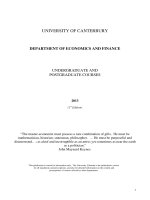
Note: 1. denotes the power curve for T = 10, and —— denotes the power curve for T = 50.
2. The first row is for the two-sided tests and the second row is for the one-sided tests.
FIGURE 14.1
Power curves under the unified approach for H
0
: ␥
0
+ ␳
0
+ ␭
0
= 1.
unified approach to get the power curves. The results are in Figure 14.1. For
the two-sided tests, the sum ␭
0
+ ␥
0
+ ␳
0
under the alternative hypothesis

ranges from 0.65 to 1.35 with a
0.7
200
increment; for the one-sided test with
H
1
: ␭
0
+ ␥
0
+ ␳
0
< 1, the sum ␭
0
+ ␥
0
+ ␳
0
ranges from 0.65 to 1.0 with a
0.35
200
increment. From Figure 14.2, we can see that the empirical sizes
18
are close to
the theoretical ones and the tests are more powerful when T = 50 than those
for the small T = 10. The power seemsreasonable for thelarge T = 50.We run
additional simulations where we use the corresponding estimation method
without any transformation. Figure 14.2 is the counterparts
19
of Table 14.1.

18
For the empirical size, the T = 10 case has 2.4%, 2.2%, 9.1%, and 8.8% from the first row to
the second row, and the T = 50 case has 1.6%, 1.7%, 6.5%, and 5.8%. As the significance level
are 1%, 1%, 5%, and 5% correspondingly, a larger T will yield empirical sizes closer to the
theoretical values.
19
For the first row in Table 14.2, when the sum ␭
0
+ ␥
0
+ ␳
0
is much larger than 1 (i.e., the
process is explosive), the estimates might not be available due to overflow without the unified
transformation. Hence, for the two-sided power curves, we allow the sum only up to 1.3.

P1: NARESH CHANDRA
November 12, 2010 18:3 C7035 C7035˙C014
A Unified Estimation Approach for Spatial Dynamic Panel Data Models 417
0.5 0.6 0.7 0.8 0.9 1 1.1 1.2 1.3 1.4 1.5
0
0.1
0.2
0.3
0.4
0.5
0.6
0.7
0.8
0.9

1
sum
α =1%
0.5 0.6 0.7 0.8 0.9 1 1.1 1.2 1.3 1.4 1.5
0
0.1
0.2
0.3
0.4
0.5
0.6
0.7
0.8
0.9
1
sum
α =5%
0.5 0.55 0.6 0.65 0.7 0.75 0.8 0.85 0.9 0.95 1
0
0.1
0.2
0.3
0.4
0.5
0.6
0.7
0.8
0.9
1
sum

α=1%
0.5 0.55 0.6 0.65 0.7 0.75 0.8 0.85 0.9 0.95 1
0
0.1
0.2
0.3
0.4
0.5
0.6
0.7
0.8
0.9
1
sum
α=5%
Note: 1. denotes the power curve for T = 10, and —— denotes the power curve for T = 50.
2. The first row is for the two-sided tests and the second row is for the one-sided tests.
FIGURE 14.2
Power curves under Yu, de Jong, and Lee (2007) for H
0
: ␥
0
+ ␳
0
+ ␭
0
= 1.
We can see that, when ␭
0
+␥

0
+␳
0
< 1, the test is more powerful by using the
corresponding method without any transformation; when ␭
0
+ ␥
0
+ ␳
0
> 1,
the power curves are irregular and we need to rely on the unified approach
for the inferences.
20
14.5 Conclusion
This chapter establishes asymptotic properties of QMLEs for SDPD models
with both time and individual fixed effects when both the number of individ-
uals nandthenumberoftimeperiods T can be large.Insteadofusingdifferent
20
For the empirical size, the T = 10 case has 34.8%, 0.3%, 44.9%, and 1.5% from the first row to
the second row in Table 14.2, and the T = 50 case has 1.1%, 0.8%, 4%, and 4%. Hence, when T
is small, the empirical sizes could be far away from the theoretical values.

P1: NARESH CHANDRA
November 12, 2010 18:3 C7035 C7035˙C014
418 Handbook of Empirical Economics and Finance
estimation methods depending on whether the DGP has time effects or not
and whether the DGP is stable or not, we propose a data transformation ap-
proachtoeliminateboththetimeeffectsandthepossibleunstableorexplosive
effects. The transformation is motivated by the possible co-integration rela-

tionship in the SDPD model, which is implied by the unit eigenvalues in the
spatial weights matrix W
n
. Unlike the co-integration in the multi-variate time
series, the co-integrating vector is known and does not need to be estimated.
With the proposed data transformation, the possible unstable or explosive
components and time effects can be eliminated.
Thetransformationusestheco-integratingmatrix.Theeffectivesamplesize
n
∗
after transformation corresponds to the co-integration rank, which is the
number of eigenvalues not equal to the unity. This transformation isof partic-
ular value when the process may contain explosive roots, as usual estimation
methods can be poorly performed under such a situation. For the unified ap-
proach, when T is relatively larger than n
∗
, the estimators are
√
n
∗
T consistent
and asymptotically centered normal; when n
∗
is asymptotically proportional
to T, the estimators are
√
n
∗
T consistent and asymptotically normal, but the
limit distribution is not centered around 0; when T is relatively smaller than

n
∗
, the estimators are consistent with rate T and have a degenerate limit dis-
tribution. We also propose a bias correction for our estimators. We show that
when T grows faster than n
∗1/3
, the correction will asymptotically eliminate
the bias and yield a centered confidence interval. Monte Carlo experiments
have demonstrated a desirable finite sample performance of the estimator. A
test statistic for testing possible spatial co-integration is also considered. In
Lee and Yu (2010b), this unified estimation approach is applied to study the
market integration in Keller and Shiue (2007) with the SDPD model and test
for the spatial co-integration.
Appendices
A Some Notes
A.1 The Eigenvalues of A
n
:Three Cases of the DGP
From Subsection 14.2.1, the eigenvalues matrix of A
n
can be decomposed as
D
n
=
␥
0
+␳
0
1−␭
0

J
n
+
˜
D
n
, where J
n
= diag{1
m
n
, 0, ···, 0} and
˜
D
n
= diag{0, ···, 0,
d
n,m
n
+1
, ···,d
nn
} with |d
ni
| < 1. Hence, A
h
n
= (
␥
0

+␳
0
1−␭
0
)
h
R
n
J
n
R
−1
n
+ B
h
n
with B
h
n
=
R
n
˜
D
h
n
R
−1
n
.Asd

ni
=
␥
0
+␳
0
␻
ni
1−␭
0
␻
ni
, the derivative of d
ni
=
␥
0
+␳
0
␻
ni
1−␭
0
␻
ni
as a function of ␻
ni
is
∂(
␥

0
+␳
0
␻
ni
1−␭
0
␻
ni
)
∂␻
ni
=
␳
0
+␥
0
␭
0
(1−␭
0
␻
ni
)
2
. Thus, d
ni
is a monotonicfunction of ␻
ni
. Our settingas-

sumes that |d
ni
| < 1 whenever d
ni
= 1. This requirement can be satisfied with
appropriaterestriction on the parameter space of ␳
0
, ␥
0
and ␭
0
as shownbelow.
The case with ␳
0
+ ␥
0
␭
0
= 0 implies that d
ni
is a constant function of ␻
ni
.
As |␭
0
| < 1 (implied by Assumptions 1 and 3), the derivative is zero if and

P1: NARESH CHANDRA
November 12, 2010 18:3 C7035 C7035˙C014
A Unified Estimation Approach for Spatial Dynamic Panel Data Models 419

only if ␳
0
+ ␥
0
␭
0
= 0, i.e., ␳
0
=−␭
0
␥
0
.Inthis situation, d
ni
=
␥
0
+␳
0
␻
ni
1−␭
0
␻
ni
= ␥
0
,
and all |d
ni

| < 1if|␥
0
| < 1.
21
The d
ni
is a strictly increasing function of ␻
ni
if
and only if ␳
0
+ ␭
0
␥
0
> 0; otherwise it is a strictly decreasing function of ␻
ni
when ␳
0
+ ␭
0
␥
0
< 0. Let ␥
0
+ ␳
0
+ ␭
0
= 1 +a, where a is a constant. We have

the stable case when ␥
0
+ ␳
0
+ ␭
0
< 1; the spatial cointegration case when
␥
0
+␳
0
+␭
0
= 1 but ␥
0
= 1; and the explosive case when ␥
0
+␳
0
+␭
0
> 1. The
condition ␳
0
+ ␥
0
␭
0
> 0(< 0) is equivalent to (1 − ␥
0

)(1 − ␭
0
) > −a (< −a)
because (1 −␥
0
)(1 −␭
0
) = ␳
0
+ ␥
0
␭
0
− a.
Assume that d
ni
is an increasing function of ␻
ni
.AsW
n
is row-normalized,
−1 ≤ ␻
ni
≤ 1 for all i.With the relation d
ni
=
␥
0
+␳
0

␻
ni
1−␭
0
␻
ni
on [−1, 1], d
ni
=
␥
0
−␳
0
1+␭
0
at ␻
ni
=−1, and d
ni
=
␥
0
+␳
0
1−␭
0
at ␻
ni
= 1. Hence, the smallest eigenvalue of A
n

will be greater than or equal to
␥
0
−␳
0
1+␭
0
, and the largest eigenvalue will occur at
␻
ni
= 1. Hence, the possible range of d
ni
with ␻
ni
in [−1, 1] is [
␥
0
−␳
0
1+␭
0
,
␥
0
+␳
0
1−␭
0
].
The smallest eigenvalue of A

n
will be greater than −1if
␥
0
− ␳
0
1 + ␭
0
> −1 ⇔ 1 +␥
0
+ ␭
0
> ␳
0
⇔ 1 − ␳
0
> −
a
2
.
Also, whenever ␻
ni
<
1−␥
0
␳
0
+␭
0
, the corresponding d

ni
< 1. This is so, because the
critical value ␻
∗
such that
␥
0
+␳
0
␻
∗
1−␭
0
␻
∗
= 1isat␻
∗
=
1−␥
0
␳
0
+␭
0
= 1 −
a
(␳
0
+␭
0

)
.
In summary, for any eigenvalue ␻
ni
of W
n
(with |␻
ni
|≤1), the correspond-
ing eigenvalue of A
n
is d
ni
=
␥
0
+␳
0
␻
ni
1−␭
0
␻
ni
. Under the situation(1−␥
0
)(1−␭
0
) > −a,
we have d

ni
< 1if␻
ni
< 1 −
a
␳
0
+␭
0
; and d
ni
> −1if1− ␳
0
> −
a
2
.
Hence, we have the following sufficient conditions for three cases in our
studies. Assume that |␭
0
| < 1 and (1 −␥
0
)(1 −␭
0
) > −a.
1. Stable case: a < 0. If ␳
0
+ ␭
0
> 0, all d

ni
≤ 1 (because ␻
ni
< 1 −
a
␳
0
+␭
0
); if
1 − ␳
0
> −
a
2
, −1 < d
ni
.
2. Spatial co-integration case: a = 0. When ␻
ni
= 1, d
ni
= 1; when ␻
ni
< 1
and 1 − ␳
0
> 0, then |d
ni
| < 1.

3. Explosive case: a > 0. When ␻
ni
= 1, d
ni
> 1; when ␻
ni
< 1 −
a
␳
0
+␭
0
=
1−␥
0
␳
0
+␭
0
, |d
ni
| < 1; furthermore, with 1 −␳
0
> −
a
2
, |d
ni
| < 1.
A.2 Decomposition

From Equation 14.2, by iterative substitution, we have
Y
nt
= A
t+1
n
Y
n,−1
+
t

h=0
A
h
n
S
−1
n
(c
n0
+ X
n,t−h
␤
0
+ V
n,t−h
+ ␣
t−h,0
l
n

).
21
For this special case, the model becomes Y
nt
= ␥
0
Y
n,t−1
+S
−1
n
(X
nt
␤
0
+c
n0
+␣
t0
l
n
+V
nt
). Hence,
this case is Y
nt
= ␥
0
Y
n,t−1

+ S
−1
n
X
nt
␤
0
+
␣
t0
1−␭
0
l
n
+ ⑀
nt
, where ⑀
nt
= ␭
0
W
n
⑀
nt
+ c
n0
+ V
nt
has the
panel disturbance structure in Kapoor, Kelejian, and Prucha (2007). This model is close to the

one considered in Su and Yang (2007) except for the resulting regressor term.

P1: NARESH CHANDRA
November 12, 2010 18:3 C7035 C7035˙C014
420 Handbook of Empirical Economics and Finance
As S
−1
n
l
n
=
1
1−␭
0
l
n
and A
n
= S
−1
n
(␥
0
I
n
+ ␳
0
W
n
) = (␥

0
I
n
+ ␳
0
W
n
)S
−1
n
, using
W
n
l
n
= l
n
,wehave A
h
n
S
−1
n
l
n
=
1
1−␭
0
(

␥
0
+␳
0
1−␭
0
)
h
l
n
.ByA
h
n
= (
␥
0
+␳
0
1−␭
0
)
h
R
n
J
n
R
−1
n
+ B

h
n
and R
n
J
n
R
−1
n
S
−1
n
= S
−1
n
R
n
J
n
R
−1
n
=
1
1−␭
0
R
n
J
n

R
−1
n
(see Proposition B.4 in Yu, de
Jong, and Lee 2007), the above equation can be written as
Y
nt
= A
t+1
n
Y
n,−1
+
t

h=0
B
h
n
S
−1
n
(c
n0
+ X
n,t−h
␤
0
+ V
n,t−h

) +
1
1 − ␭
0
t

h=0

␥
0
+ ␳
0
1 − ␭
0

h
×␣
t−h,0
l
n
+
1
1 − ␭
0
t

h=0

␥
0

+ ␳
0
1 − ␭
0

h
R
n
J
n
R
−1
n
(c
n0
+ X
n,t−h
␤
0
+ V
n,t−h
).
For A
t+1
n
Y
n,−1
,wehave A
t+1
n

Y
n,−1
= (
␥
0
+␳
0
1−␭
0
)
t+1
R
n
J
n
R
−1
n
Y
n,−1
+B
t+1
n
Y
n,−1
, where
B
t+1
n
Y

n,−1
=
∞

h=t+1
B
h
n
S
−1
n
(c
n0
+ X
n,t−h
␤
0
+ V
n,t−h
) +
1
1 − ␭
0
∞

h=t+1
␣
t−h,0
B
h

n
l
n
,
using B
n
A
n
= B
2
n
and B
n
S
−1
n
= S
−1
n
B
n
. The item with B
h
n
l
n
is zero. Because R
n
is the eigenvectors matrix of W
n

and its first column is l
n
,wehave R
−1
n
l
n
= e
n1
which is the first unit vector. As
˜
D
n
e
n1
= 0, it follows that B
n
l
n
= 0. Hence,
we can decompose Y
nt
as Y
nt
= Y
u
nt
+ Y
s
nt

+ Y
␣
nt
, which is Equation 14.3.
The Y
s
nt
represents a stable component as the eigenvalues of B
n
can be
less than unity in absolute value for many parameter values (see
Appendix A.1). The Y
␣
nt
captures the component due to time dummies. As
|
␥
0
+␳
0
1−␭
0
| < 1ifand only if −1 < ␥
0
+ ␳
0
+ ␭
0
< 1 because ␭
0

< 1, Y
u
nt
is also
stable when ␥
0
+␳
0
+␭
0
< 1. But when ␥
0
+␳
0
+␭
0
= 1(> 1), then
␥
0
+␳
0
1−␭
0
= 1
(> 1) and Y
u
nt
may represent the unstable or explosive components.
A.3 Data Transformation
We can transform Equation 14.1 by I

n
− W
n
into Equation 14.4, where the
remaining (I
n
− W
n
)c
n0
can be regarded as the individual effects. A spe-
cial feature of the transformed Equation 14.4 is that the variance matrix of
(I
n
− W
n
)V
nt
is equal to ␴
2
0

n
≡ ␴
2
0
(I
n
− W
n

)(I
n
− W
n
)

, which is singular.
Hence, there is a linear dependence among the elements of (I
n
− W
n
)V
nt
.An
effective estimation method shall eliminate the linear dependence. This can
be donewith the eigenvalues and eigenvectors decomposition (see,e.g., Theil
1971, Chapter 6).
Let [F
n
,H
n
]bethe orthonormalmatrix of eigenvectors and 
n
be thediago-
nalmatrixofnonzero eigenvalues of 
n
suchthat
n
F
n

= F
n

n
and
n
H
n
= 0.
That is, the columns of F
n
consist of eigenvectors of nonzero eigenvalues and
those of H
n
are for zero-eigenvalues of 
n
. Let n
∗
be the number of nonzero
eigenvalues. The F
n
is an n ×n
∗
matrix and 
n
is an n
∗
×n
∗
diagonal matrix.

Thus,

n
F
n
= F
n

n
,F

n
F
n
= I
n
∗
, 
n
H
n
= 0,H

n
H
n
= I
n−n
∗
,

F

n
H
n
= 0,F
n
F

n
+ H
n
H

n
= I
n
,F
n

n
F

n
= 
n
.
(14.28)

P1: NARESH CHANDRA

November 12, 2010 18:3 C7035 C7035˙C014
A Unified Estimation Approach for Spatial Dynamic Panel Data Models 421
Because 
n
H
n
= 0, it implies that (I
n
− W
n
)

H
n
= 0. In turn, W
n
(I
n
− W
n
) =
W
n
(F
n
F

n
+H
n

H

n
)(I
n
−W
n
) = W
n
F
n
F

n
(I
n
−W
n
).Denote W
∗
n
= 
−1/2
n
F

n
W
n
F

n

1/2
n
which is a n
∗
× n
∗
matrix. This matrix can be regarded as a spatial weights
matrix for the following transformed equation:
Y
∗
nt
= ␭
0
W
∗
n
Y
∗
nt
+ ␥
0
Y
∗
n,t−1
+ ␳
0
W
∗

n
Y
∗
n,t−1
+ X
∗
nt
␤
0
+ c
∗
n0
+ V
∗
nt
, (14.29)
where Y
∗
nt
= 
−1/2
n
F

n
(I
n
−W
n
)Y

nt
and other variables are defined correspond-
ingly. Note that this transformed Y
∗
nt
is an n
∗
dimensional vector. Hence, after
the transformation, the observations at time period t have only n
∗
degrees
of freedom. Equation 14.29 shall provide the structural parameters for esti-
mation. This equation is in the format of a typical SAR model in panel data,
where the number of observations is n
∗
T.
A.4 Determinant and Inverse of S
∗
n
(␭) ≡ I
n
∗
− ␭W
∗
n
We note that S
∗
n
= 
−1/2

n
F

n
S
n
F
n

1/2
n
.Let␮be ascalar. Because(I
n
−W
n
)·H
n
= 0,
[F
n
,H
n
]

(␮I
n
− W
n
)[F
n

,H
n
]
=

␮I
n
∗
− F

n
W
n
F
n
−F

n
W
n
H
n
−H

n
W
n
F
n
␮I

n−n
∗
− H

n
W
n
H
n

=

␮I
n
∗
− F

n
W
n
F
n
−F

n
W
n
H
n
0 (␮ −1)I

n−n
∗

.
Hence, |␮I
n
−W
n
|=(␮−1)
n−n
∗
|␮I
n
∗
−F

n
W
n
F
n
|. Because |␮I
n
∗
−W
∗
n
|=|␮I
n
∗

−

−1/2
n
F

n
W
n
F
n

1/2
n
|=|␮I
n
∗
− F

n
W
n
F
n
|, |␮I
n
− W
n
|=(␮ − 1)
n−n

∗
|␮I
n
∗
− W
∗
n
|.
As W
n
has (n − n
∗
) unit eigenvalues, the eigenvalues of W
∗
n
are exactly the
remaining eigenvalues of W
n
, which are less than unity in the absolute value.
Furthermore,
|S
∗
n
(␭)|=
1
(1 −␭)
n−n
∗
|S
n

(␭)|. (14.30)
Thus, the tractability in computing the determinant of S
∗
n
(␭)isexactly that of
S
n
(␭).WhenW
n
isconstructedas aweightsmatrix thatisrow-normalizedfrom
an original symmetric matrix, Ord (1975) has suggested a computationally
tractable method for the evaluation of |S
n
(␭)|at various ␭ for the ML method.
This is useful for evaluating the determinant of S
∗
n
(␭) even though the row
sums of W
∗
n
may not even be unity.
Furthermore, a SAR model is an equilibrium model in the sense that the
observed outcomes are determined by the equation. That is, the matrix S
∗
n
(␭)
shall be invertible. For the transformed equation (Equation 14.29), S
∗
n

(␭)is
invertible as long as the original matrices S
n
(␭)inEquation 14.1 is invertible.
We can see that
S
∗−1
n
(␭) = 
−1/2
n
F

n
S
−1
n
(␭)F
n

1/2
n
, (14.31)

P1: NARESH CHANDRA
November 12, 2010 18:3 C7035 C7035˙C014
422 Handbook of Empirical Economics and Finance
because
S
∗

n
(␭) · 
−1/2
n
F

n
S
−1
n
(␭)F
n

1/2
n
= 
−1/2
n
F

n
S
n
(␭)F
n
F

n
S
−1

n
(␭)F
n

1/2
n
= 
−1/2
n
F

n
S
n
(␭)(I
n
− H
n
H

n
)S
−1
n
(␭)F
n

1/2
n
= I

n
∗
− 
−1/2
n
F

n
S
n
(␭)H
n
H

n
S
−1
n
(␭)F
n

1/2
n
= I
n
∗
,
as H

n

W
n
= H

n
, H

n
S
−1
n
(␭) =
1
1−␭
H

n
and H

n
F
n
= 0.
A.5 About tr(G
∗
n
(␭))
We have G
∗
n

(␭) = 
−1/2
n
F

n
G
n
(␭)F
n

1/2
n
.Thisis sobecause,fromEquation14.31,
G
∗
n
(␭) = W
∗
n
S
−1∗
n
(␭) = 
−1/2
n
F

n
W

n
F
n
F

n
S
−1
n
(␭)F
n

1/2
n
= 
−1/2
n
F

n
W
n
(I
n
− H
n
H

n
)S

−1
n
(␭)F
n

1/2
n
= 
−1/2
n
F

n
W
n
S
−1
n
(␭)F
n

1/2
n
− 
−1/2
n
F

n
W

n
H
n
H

n
S
−1
n
(␭)F
n

1/2
n
= 
−1/2
n
F

n
W
n
S
−1
n
(␭)F
n

1/2
n

= 
−1/2
n
F

n
G
n
(␭)F
n

1/2
n
,
because H

n
S
−1
n
(␭)F
n
=
1
1−␭
H

n
F
n

= 0. Hence,
tr(G
∗
n
(␭)) = tr(F

n
G
n
(␭)F
n
) = tr[G
n
(␭)(I
n
− H
n
H

n
)] = tr(G
n
(␭)) −
n −n
∗
1 − ␭
,
(14.32)
where the last equality holds because H


n
W
n
= H

n
and H

n
S
−1
n
(␭) =
1
1−␭
H

n
implies that
tr(G
n
(␭)H
n
H

n
) = tr(H

n
G

n
(␭)H
n
) = tr(H

n
W
n
S
−1
n
(␭)H
n
) =
1
1 − ␭
tr(H

n
H
n
)
=
n −n
∗
1 − ␭
.
As G
∗2
n

(␭) = 
−1/2
n
F

n
G
n
(␭)F
n
F

n
G
n
(␭)F
n

1/2
n
,wehave
tr(G
∗2
n
(␭)) = tr(F

n
G
n
(␭)F

n
F

n
G
n
(␭)F
n
) = tr(G
n
(␭)F
n
F

n
G
n
(␭)F
n
F

n
)
= tr(G
n
(␭)(I
n
− H
n
H


n
)G
n
(␭)(I
n
− H
n
H

n
)).
Using H

n
G
n
(␭) =
1
(1−␭)
H

n
and H

n
H
n
= I
n−n

∗
,wehave [G
n
(␭)(I
n
− H
n
H

n
)]
2
=
[G
n
(␭)]
2
[I
n
− H
n
H

n
] and
tr(G
∗2
n
(␭)) = tr(G
2

n
(␭)) −
n −n
∗
(1 −␭)
2
, (14.33)
because H

n
G
2
n
(␭)H
n
=
1
(1−␭)
2
H

n
H
n
=
1
(1−␭)
2
I
n−n

∗
.Interms of the eigenval-
ues of W
n
,asW
n
= R
n
ϖR
−1
n
, tr(G
∗
n
(␭)) =

n
j=m
n
+1
ϖ
nj
1−␭ϖ
nj
and tr(G
∗2
n
(␭)) =

n

j=m
n
+1
ϖ
2
nj
(1−␭ϖ
nj
)
2
.

P1: NARESH CHANDRA
November 12, 2010 18:3 C7035 C7035˙C014
A Unified Estimation Approach for Spatial Dynamic Panel Data Models 423
Also, as J
∗
n
= (I
n
−W
n
)


+
n
(I
n
−W

n
) and (I
n
−W
n
)G
n
(␭) = G
n
(␭)(I
n
−W
n
),
Equation 14.32 implies that
tr(J
∗
n
G
n
(␭)) = tr(G
n
(␭)(I
n
− W
n
)(I
n
− W
n

)

F
n

−1
n
F

n
)
= tr(G
n
(␭)F
n
F

n
) = tr(G
n
(␭)(I
n
− H
n
H

n
))
= tr(G
∗

n
(␭)). (14.34)
For J
∗
n
,wehave tr(J
∗
n
) = tr((I
n
−W
n
)

F
n

−1
n
F

n
(I
n
−W
n
)) = tr(
−1
n


n
) = n
∗
by
using Equation 14.28. The J
∗
n
is an orthogonal projector. This is so, because
J
∗
n
is symmetric and J
∗
n
J
∗
n
= (I
n
−W
n
)


+
n
(I
n
−W
n

) ·(I
n
−W
n
)


+
n
(I
n
−W
n
) =
(I
n
− W
n
)


+
n

n

+
n
(I
n

− W
n
) = (I
n
− W
n
)


+
n
(I
n
− W
n
) = J
∗
n
.
B Lemmas for Some Statistics in the Model
The following lemmas can be found in Yu, de Jong, and Lee (2008). These
lemmas provide orders for relevant terms in the score and the Hessian matrix
ofthelog-likelihoodfunction.They include also aCLT for linear andquadratic
forms of disturbances. Denote U
nt
=

∞
h=1
P

nh
V
n,t+1−h
, where {P
nh
}
∞
h=1
is a
sequence of n ×n nonstochastic square matrices.
Assumption A1 The disturbances {v
it
}, i = 1, 2, ,nand t = 1, 2, ,T,are
i.i.d. across i and t with zero mean, variance ␴
2
0
and E|v
it
|
4+␩
< ∞ for some
␩ > 0.
Assumption A2

∞
h=1
abs(P
nh
)isUB.
Assumption A3 The elements of n × 1 vector D

nt
are nonstochastic and
bounded, uniformly in n and t.
Assumption A4 n is a nondecreasing function of T and T goes to infinity.
Lemma 14.1 Under Assumptions A1 and A4, for an n × n nonstochastic matrix
B
n
, uniformly bounded in row and column sums,
1
nT
T

t=1
V

nt
B
n
V
nt
− E(
1
nT
T

t=1
V

nt
B

n
V
nt
) = O
p

1
√
nT

, (14.35)
1
n
¯
V

nT
B
n
¯
V
nT
− E(
1
n
¯
V

nT
B

n
¯
V
nT
) = O
p

1
√
nT
2

, (14.36)
and
1
nT
T

t=1
˜
V

nt
B
n
˜
V
nt
− E(
1

nT
T

t=1
˜
V

nt
B
n
˜
V
nt
) = O
p

1
√
nT

, (14.37)
where E(
1
nT

T
t=1
V

nt

B
n
V
nt
) = O(1), E(
1
n
¯
V

nT
B
n
¯
V
nT
) = O(T
−1
) and E(
1
nT

T
t=1
˜
V

nt
B
n

˜
V
nt
) = O(1).

P1: NARESH CHANDRA
November 12, 2010 18:3 C7035 C7035˙C014
424 Handbook of Empirical Economics and Finance
Lemma 14.2 Under Assumptions A1, A2, and A4,

T
n
(
¯
U

nT,−1
¯
V
nT
− E(
¯
U

nT,−1
¯
V
nT
)) = O
p


1
√
T

, (14.38)
where

T
n
E(
¯
U

nT,−1
¯
V
nT
) =

n
T
1
n
␴
2
0
tr



∞
h=1
P
nh

+ O


n
T
3

.
For the lemma that follows, we will consider the following form:
Q
nT
=
T

t=1
(U

n,t−1
V
nt
+ D

nt
V
nt

+ V

nt
B
n
V
nt
− ␴
2
0
tr(B
n
)) =
T

t=1
n

i=1
z
nt,i
,
where B
n
is a n × n nonstochastic symmetric matrix which is UB, and z
nt,i
=
(u
i,t−1
+ d

nti
)v
it
+ b
n,ii
(v
2
it
− ␴
2
0
) + 2(

i−1
j=1
b
n,i j
v
jt
)v
it
, where b
n,i j
is the (i, j)
elementofB
n
andd
nti
istheithelement of D
nt

.Then,forthemeanandvariance
of Q
nT
, ␮
Q
nT
= 0 and
␴
2
Q
nT
= T␴
4
0
tr

∞

h=1
P

nh
P
nh

+ ␴
2
0
T


t=1
D

nt
D
nt
+T


␮
4
− 3␴
4
0

n

i=1
b
2
n,ii
+ 2␴
4
0
tr(B
2
n
)

+ 2␮

3
T

t=1
n

i=1
d
nti
b
n,ii
,
where ␮
s
= Ev
s
it
for s = 3, 4.
Lemma 14.3 Under Assumptions A1, A2, A3, A4, and that B
n
is UB, if the
sequence
1
nT
␴
2
Q
nT
is bounded away from zero, then,
Q

nT
␴
Q
nT
d
→ N(0, 1).
Denote Z
nt
= (Y
n,t−1
,W
n
Y
n,t−1
,X
nt
), we are going to provide some lemmas
related to (I
n
−W
n
)
˜
Z
nt
,(I
n
−W
n
)

¯
Z
nT
and
˜
V
nt
,
¯
V
nT
of the model Equation 14.1.
Lemma 14.4 Under Assumptions 1–7, for an n ×n nonstochastic UB matrix B
n
,
1
nT
T

t=1
˜
Z

nt
(I
n
− W
n
)


B
n
(I
n
− W
n
)
˜
Z
nt
− E
1
nT
T

t=1
˜
Z

nt
(I
n
− W
n
)

B
n
(I
n

− W
n
)
˜
Z
nt
= O
p

1
√
nT

, (14.39)

P1: NARESH CHANDRA
November 12, 2010 18:3 C7035 C7035˙C014
A Unified Estimation Approach for Spatial Dynamic Panel Data Models 425
and
1
nT
T

t=1
˜
Z

nt
(I
n

− W
n
)

B
n
(I
n
− W
n
)
˜
V
nt
− E
1
nT
T

t=1
˜
Z

nt
(I
n
− W
n
)


B
n
(I
n
− W
n
)
˜
V
nt
= O
p

1
√
nT

, (14.40)
where E
1
nT

T
t=1
˜
Z

nt
(I
n

− W
n
)

B
n
(I
n
− W
n
)
˜
Z
nt
is O(1) and E
1
nT

T
t=1
˜
Z

nt
(I
n
−
W
n
)


B
n
(I
n
− W
n
)
˜
V
nt
is O

1
T

.
Lemma 14.5 If B
n
(␪
0
))
∞
< 1 (resp: B
n
(␪
0
))
1
< 1), then the row sum (resp:

column sum) of

∞
h=0
B
h
n
(␪) and

∞
h=1
hB
h−1
n
(␪) are bounded uniformly in n and
in a neighborhood of ␪
0
.
C Concentrated QML of the Transformation Approach
C.1 Reduced Form of Equation 14.1
From Equation 14.1, we have Y
nt
= S
−1
n
(Z
nt
␦
0
+c

n0
+␣
t
l
n
+ V
nt
) and W
n
Y
nt
=
G
n
Z
nt
␦
0
+ G
n
c
n0
+ ␣
t
G
n
l
n
+ G
n

V
nt
.Byusing S
−1
n
= I
n
+ ␭
0
G
n
, Y
nt
= Z
nt
␦
0
+
␭
0
G
n
Z
nt
␦
0
+S
−1
n
c

n0
+␣
t
S
−1
n
l
n
+S
−1
n
V
nt
.With S
−1
n
l
n
=
1
1−␭
0
l
n
and (I
n
−W
n
)l
n

= 0,
˜
Y
nt
=
˜
Z
nt
␦
0
+ ␭
0
G
n
˜
Z
nt
␦
0
+
˜␣
t
1 − ␭
0
l
n
+ S
−1
n
˜

V
nt
,
and
(I
n
−W
n
)
˜
Y
nt
= (I
n
−W
n
)
˜
Z
nt
␦
0
+␭
0
(I
n
−W
n
)G
n

˜
Z
nt
␦
0
+(I
n
−W
n
)S
−1
n
˜
V
nt
. (14.41)
Similarly, as W
n
˜
Y
nt
= G
n
˜
Z
nt
␦
0
+ ˜␣
t

G
n
l
n
+ G
n
˜
V
nt
,
(I
n
− W
n
)W
n
˜
Y
nt
= (I
n
− W
n
)G
n
˜
Z
nt
␦
0

+ (I
n
− W
n
)G
n
˜
V
nt
, (14.42)
because (I
n
− W
n
)G
n
l
n
=
1
1−␭
0
(I
n
− W
n
)l
n
= 0.

P1: NARESH CHANDRA
November 12, 2010 18:3 C7035 C7035˙C014
426 Handbook of Empirical Economics and Finance
C.2 FOC and SOC of the Concentrated Log-Likelihood
Denote J
∗
n
= (I
n
− W
n
)


+
n
(I
n
− W
n
) and G
∗
n
= W
∗
n
S
∗−1
n
.Byusing trG

n
(␭) −
tr(G
∗
n
(␭)) =
n−n
∗
1−␭
and tr(G
2
n
(␭)) −tr(G
∗2
n
(␭)) =
n−n
∗
(1−␭)
2
(see Appendix A.5), the
first-order derivatives of Equation 14.10 are
∂ ln L
n,T
(␪)
∂␪
=













1
␴
2
T

t=1
(J
∗
n
˜
Z
nt
)

˜
V
nt
(␪)
1
␴
2

T

t=1
((J
∗
n
W
n
˜
Y
nt
)

˜
V
nt
(␪)) − TtrG
∗
n
(␭)
1
2␴
4
T

t=1
(
˜
V


nt
(␪)J
n
˜
V
nt
(␪) − n
∗
␴
2
)












, (14.43)
and the second order derivatives are
∂
2
ln L
n,T
(␪)

∂␪∂␪

=−








1
␴
2
T

t=1
˜
Z

nt
J
∗
n
˜
Z
nt
1
␴
2

T

t=1
˜
Z

nt
J
∗
n
W
n
˜
Y
nt
1
␴
4
T

t=1
˜
Z

nt
J
∗
n
˜
V

nt
(␪)
∗
1
␴
2
T

t=1

(W
n
˜
Y
nt
)

J
∗
n
W
n
˜
Y
nt
) + Ttr((G
∗
n
(␭))
2


1
␴
4
T

t=1
(W
n
˜
Y
nt
)

J
∗
n
˜
V
nt
(␪)
∗∗−
n
∗
T
2␴
4
+
1
␴

6
T

t=1
˜
V

nt
(␪)J
∗
n
˜
V
nt
(␪)








.
(14.44)
At ␪
0
,
1
√

n
∗
T
∂ ln L
n,T
(␪
0
)
∂␪
=












1
␴
2
0
1
√
n
∗

T
T

t=1
˜
Z

nt
J
∗
n
˜
V
nt
1
␴
2
0
1
√
n
∗
T
T

t=1
(G
n
˜
Z

nt
␦
0
)

J
∗
n
˜
V
nt
+
1
␴
2
0
1
√
n
∗
T
T

t=1
(
˜
V

nt
G


n
J
∗
n
˜
V
nt
− ␴
2
0
trG
∗
n
)
1
2␴
4
0
1
√
n
∗
T
T

t=1
(
˜
V


nt
J
∗
n
˜
V
nt
− n
∗
␴
2
0
)












,
(14.45)

P1: NARESH CHANDRA

November 12, 2010 18:3 C7035 C7035˙C014
A Unified Estimation Approach for Spatial Dynamic Panel Data Models 427
which is a linear and quadratic form of
˜
V
nt
. For the information matrix,

␪
0
,nT
=
1
␴
2
0

EH
nT
0
(k+3)×1
0
1×(k+3)
0

+






0
(k+2)×(k+2)
0
(k+2)×1
0
(k+2)×1
0
1×(k+2)
1
n
∗

tr(G

n
J
∗
n
G
n
) + tr((G
∗
n
)
2
)

1
␴

2
0
n
∗
tr(J
∗
n
G
n
)
0
1×(k+2)
1
␴
2
0
n
∗
tr(J
∗
n
G
n
)
1
2␴
4
0






−






0
(k+2)×(k+2)
∗∗
1
␴
2
0
n
∗
E(G
n
¯
V
nT
)

J
∗
n
¯

Z
nT
2
␴
2
0
n
∗
E[(G
n
¯
Z
nT
␦
0
)

J
∗
n
G
n
¯
V
nT
] +
1
n
∗
T

tr(G

n
J
∗
n
G
n
) ∗
1
␴
4
0
n
∗
E(
¯
Z

nT
J
∗
n
¯
V
nT
)

1
␴

4
0
n
∗
E[(G
n
¯
Z
nT
␦
0
)

J
∗
n
¯
V
nT
]

+
1
␴
2
0
n
∗
T
tr(J

∗
n
G
n
)
1
T
1
␴
4
0






.
C.3 About −
1
n
∗
T
∂
2
ln L
nT
(␪)
∂␪∂␪


Denote ␪ − ␪
0
 as the Euclidean norm of ␪ − ␪
0
, and 
1
as a neighborhood
of ␪
0
, then, we have
1
n
∗
T
∂
2
ln L
nT
(␪)
∂␪∂␪

−
1
n
∗
T
∂
2
ln L
nT

(␪
0
)
∂␪∂␪

=␪ −␪
0
·O
p
(1), (14.46)
1
n
∗
T
∂
2
ln L
nT
(␪
0
)
∂␪∂␪

+ 
␪
0
,nT
= O
p


1
√
n
∗
T

, (14.47)
sup
␪∈




1
n
∗
T
∂
2
ln L
nT
(␪)
∂␪∂␪

−
1
n
∗
T
E

∂
2
ln L
nT
(␪)
∂␪∂␪





ij
= O
p

1
√
n
∗
T

, (14.48)
and
sup
␪∈
1





1
n
∗
T
E
∂
2
ln L
nT
(␪)
∂␪∂␪

+ 
␪
0
,nT




ij
= sup
␪∈
1
␪ − ␪
0
·O(1) (14.49)
for all i, j = 1, 2, ···,k+ 4. These are Equation A.11 to Equation A.14 in Yu,
de Jong, and Lee (2008).
DProofs for Claims and Theorems

D.1Proof of nonsingularity of the information matrix
The result can be proved by using an argument by contradiction. For 
␪
0
≡
lim
T→∞

␪
0
,nT
, where 
␪
0
,nT
is Equation 14.12, we shall prove that 
␪
0
␣ = 0

P1: NARESH CHANDRA
November 12, 2010 18:3 C7035 C7035˙C014
428 Handbook of Empirical Economics and Finance
implies ␣ = 0, where ␣ = (␣

1
, ␣
2
, ␣
3

)

, ␣
2
, ␣
3
are scalars and ␣
1
is (k + 2) × 1
vector. If this is true, then, columns of 
␪
0
would be linear independent sothat

␪
0
would be nonsingular. Denote H
␦
= plim
T→∞
1
n
∗
T

T
t=1
˜
Z


nt
J
∗
n
˜
Z
nt
, H
␦␭
=
plim
T→∞
1
n
∗
T

T
t=1
˜
Z

nt
J
∗
n
G
n
˜
Z

nt
␦
0
, H
␭␦
= H

␦␭
and H
␭
= plim
T→∞
1
n
∗
T

T
t=1
(G
n
˜
Z
nt
␦
0
)

J
∗

n
G
n
˜
Z
nt
␦
0
. Then

␪
0
=
1
␴
2
0






H
␦
H
␦␭
0
(k+2)×1
H

␭␦
EH
␭
+ lim
n→∞
␴
2
0
n
∗

tr(G

n
J
∗
n
G
n
) + tr((G
∗
n
)
2
)

lim
n→∞
1
n

∗
tr( J
∗
n
G
n
)
0
1×(k+2)
lim
n→∞
1
n
∗
tr( J
∗
n
G
n
)
1
2␴
2
0







.
Hence, 
␪
0
␣ = 0 implies
H
␦
× ␣
1
+ H
␦␭
× ␣
2
= 0,
1
␴
2
0
H
␭␦
× ␣
1
+

1
␴
2
0
H
␭

+ lim
n→∞
1
n
∗

tr(G

n
J
∗
n
G
n
) + tr((G
∗
n
)
2
)


×␣
2
+ lim
n→∞
1
␴
2
0

n
∗
tr(J
∗
n
G
n
) × ␣
3
= 0,
lim
n→∞
1
n
∗
tr(J
∗
n
G
n
) × ␣
2
+
1
2␴
2
0
× ␣
3
= 0.

From the first equation, ␣
1
=−(H
␦
)
−1
H
␦␭
× ␣
2
;from the third equation,
␣
3
=−2lim
n→∞
␴
2
0
n
∗
tr(J
∗
n
G
n
) × ␣
2
.Byeliminating ␣
1
and ␣

3
, the remaining
equation becomes

1
␴
2
0

H
␭
− H
␭␦
H
−1
␦
H
␦␭


+ lim
n→∞
1
n
∗

tr(G

n
J

∗
n
G
n
) + tr((G
∗
n
)
2
) − 2
tr
2
(J
∗
n
G
n
)
n
∗

× ␣
2
= 0.
Using Equation 14.34 and that J
∗
n
is idempotent, denote C
n
= G

∗
n
−
tr(G
∗
n
)
n
∗
,we
have
tr(G

n
J
∗
n
G
n
) + tr((G
∗
n
)
2
) − 2
tr
2
(J
∗
n

G
n
)
n
∗
= tr(G
∗
n
G
∗
n
) + tr((G
∗
n
)
2
) − 2
tr
2
(G
∗
n
)
n
∗
=
1
2
tr(C


n
+C
n
)(C

n
+C
n
)

,
which is nonnegative. Hence, if the limit of EH
nT
is nonsingular or the limit
of
1
n
∗
(tr(G
∗
n
G
∗
n
) + tr((G
∗
n
)
2
) − 2

tr
2
(G
∗
n
)
n
∗
)isnonzero, we have ␣
2
= 0 and hence
␣ = 0. This proves the nonsingularity of 
␪
0
. 

P1: NARESH CHANDRA
November 12, 2010 18:3 C7035 C7035˙C014
A Unified Estimation Approach for Spatial Dynamic Panel Data Models 429
D.2Proof of Theorem 14.1
To prove
1
n
∗
T
ln L
n,T
(␪) − Q
n,T
(␪)

p
→ 0 uniformly in ␪ in any compact parameter
space :
From
˜
V
nt
(␪) ≡ S
n
(␭)
˜
Y
nt
−
˜
Z
nt
␦ − ˜␣
t
l
n
and
˜
V
nt
= S
n
˜
Y
nt

−
˜
Z
nt
␦
0
− ˜␣
t0
l
n
, using
J
∗
n
l
n
= 0,wehave J
∗
n
˜
V
nt
(␪) = J
∗
n
˜
V
nt
−(␭ −␭
0

)J
∗
n
W
n
˜
Y
nt
− J
∗
n
˜
Z
nt
(␦ −␦
0
). As 
is compact and ␴
2
is bounded away from zero in ,byLemma 14.1 and 14.4,
1
n
∗
T
ln L
n,T
(␪) − Q
n,T
(␪)
=−

1
2␴
2

1
n
∗
T
T

t=1
˜
V

nt
(␪)J
∗
n
˜
V
nt
(␪) −
1
n
∗
T
E
T

t=1

˜
V

nt
(␪)J
∗
n
˜
V
nt
(␪)

p
→ 0
uniformly in ␪ in .
To prove Q
n,T
(␪) is uniformly equicontinuous in ␪ in any compact parameter
space :
For Q
n,T
(␪)inEquation 14.11, as J
∗
n
˜
V
nt
(␪) = J
∗
n

[S
n
(␭)
˜
Y
nt
−
˜
Z
nt
␦] and
˜
Y
nt
=
S
−1
n
˜
Z
nt
␦
0
+ S
−1
n
˜
V
nt
+

˜␣
t0
1−␭
0
l
n
,
J
∗
n
˜
V
nt
(␪) = J
∗
n
[S
n
(␭)S
−1
n
˜
Z
nt
␦
0
−
˜
Z
nt

␦ + S
n
(␭)S
−1
n
˜
V
nt
]
because J
∗
n
l
n
= 0. Hence,
E
1
n
∗
T
T

t=1
˜
V

nt
(␪)J
∗
n

˜
V
nt
(␪) =
1
n
∗
T
E
T

t=1
(S
n
(␭)S
−1
n
˜
Z
nt
␦
0
−
˜
Z
nt
␦)

J
∗

n
(S
n
(␭)
×S
−1
n
˜
Z
nt
␦
0
−
˜
Z
nt
␦) +
1
n
∗
T − 1
T
␴
2
0
tr
×(S
−1

n

S

n
(␭)J
∗
n
S
n
(␭)S
−1
n
) +
2
n
∗
T
E
T

t=1
×(S
n
(␭)S
−1
n
˜
Z
nt
␦
0

−
˜
Z
nt
␦)

J
∗
n
S
n
(␭)S
−1
n
˜
V
nt
. (14.50)
With these terms, similar to Lee and Yu (2010a), it can be shown that Q
n,T
(␪)
is uniformly equicontinuous in ␪ in any compact parameter space .
To prove the identification:
As tr J
∗
n
= n
∗
,E


T
t=1
˜
V

nt
J
∗
n
˜
V
nt
= n
∗
(T − 1)␴
2
0
from Lemma 14.1. Hence,
1
n
∗
T
ElnL
n,T
(␪)−
1
n
∗
T
ElnL

n,T
(␪
0
) =−
1
2
(ln␴
2
−ln ␴
2
0
)+
1
n
∗
ln |S
n
(␭)|−
1
n
∗
ln |S
n
|−
n−n
∗
n
∗
(ln(1 − ␭) − ln(1 − ␭
0

)) − (
1
2␴
2
1
n
∗
T

T
t=1
E
˜
V

nt
(␪)J
∗
n
˜
V
nt
(␪) −
T−1
2T
). By us-
ing S
n
(␭)S
−1

n
= I
n
+ (␭
0
− ␭)G
n
,from Equation 14.50,
1
n
∗
T
ElnL
n,T
(␪) −
1
n
∗
T
ElnL
n,T
(␪
0
) = T
1,n
(␭, ␴
2
) −
1
2␴

2
T
2,n,T
(␦, ␭) + O(T
−1
), where
T
1,n
(␭, ␴
2
) =−
1
2
(ln␴
2
− ln ␴
2
0
) +
1
n
∗
ln |S
n
(␭)|−
1
n
∗
ln |S
n

|−
n −n
∗
n
∗
×(ln(1 −␭) −ln(1 −␭
0
)) −
1
2␴
2
(␴
2
n
(␭) − ␴
2
),

P1: NARESH CHANDRA
November 12, 2010 18:3 C7035 C7035˙C014
430 Handbook of Empirical Economics and Finance
and
T
2,n,T
(␦, ␭) =
1
n
∗
T
T


t=1
E{[
˜
Z
nt
(␦
0
− ␦) + (␭
0
− ␭)G
n
˜
Z
nt
␦
0
]

J
∗
n
×[
˜
Z
nt
(␦
0
− ␦) + (␭
0

− ␭)G
n
˜
Z
nt
␦
0
]},
where ␴
2
n
(␭) =
␴
2
0
n
∗
tr(S
−1
n
S

n
(␭)J
∗
n
S
n
(␭)S
−1

n
). Consider the pure spatial process
Y
nt
= ␭
0
W
n
Y
nt
+␣
t
l
n
+V
nt
forasingleperiod t.Withsimilardatatransformation
as in Equation 14.5, the log-likelihood function of this process is
ln L
p,n
(␭, ␴
2
) =−
n
∗
2
ln 2␲ −
n
∗
2

ln ␴
2
− (n −n
∗
) ln(1 −␭) + ln |S
n
(␭)|
−
1
2␴
2
V

nt
(␭)J
∗
n
V

nt
(␭), (14.51)
where V
nt
(␭) = S
n
(␭)Y
nt
. Let E
p
(·)bethe expectation operator for Y

nt
based
on this pure spatial autoregressive process. It follows that
E
p
(
1
n
∗
ln L
p,n
(␭, ␴
2
)) − E
p
(
1
n
∗
ln L
p,n
(␭
0
, ␴
2
0
))
=−
1
2

(ln␴
2
− ln ␴
2
0
) +
1
n
∗
ln |S
n
(␭)|−
1
n
∗
ln |S
n
|−
n −n
∗
n
∗
(ln(1 −␭)
− ln(1 −␭
0
)) −
1
2␴
2
(␴

2
n
(␭) − ␴
2
),
which equals to T
1,n
(␭, ␴
2
). By the information inequality, ln L
p,n
(␭, ␴
2
) −
ln L
p,n
(␭
0
, ␴
2
0
) ≤ 0. Thus, T
1,n
(␭, ␴
2
) ≤ 0 for any (␭, ␴
2
).
For T
2,n,T

(␦, ␭), it is a quadratic function of ␦ and ␭. Under the assumed
condition that lim
T→∞
EH
nT
is nonsingular, lim
T→∞
T
2,n,T
(␦, ␭) > 0 when-
ever (␦, ␭) = (␦
0
, ␭
0
). So, (␦, ␭)isglobally identified. Given ␭
0
, ␴
2
0
is also the
unique maximizer of T
1,n
(␭
0
, ␴
2
) for any given n
∗
.Inthe event that n
∗

→∞,
␴
2
0
is the unique maximizer of lim
T→∞
T
1,n
(␭
0
, ␴
2
).Hence, (␦, ␭, ␴
2
)isglobally
identified.
By combining the results above together, the consistency follows. 
D.3Proof of Theorem 14.2
When the limit of EH
nT
is singular, ␦
0
and ␭
0
cannot be identified from
T
2,n,T
(␦, ␭)inAppendix D.2. Identification requires that the limit of T
1,n
(␭, ␴

2
)
is strictly less than zero whenever (␭, ␴
2
) = (␭
0
, ␴
2
0
). Thus, the identification
will just be from the likelihood function Equation 14.51. By concentrating out

P1: NARESH CHANDRA
November 12, 2010 18:3 C7035 C7035˙C014
A Unified Estimation Approach for Spatial Dynamic Panel Data Models 431
␴
2
in Equation 14.51, we have the concentrated log-likelihood function
ln L
p,n
(␭) =−
n
∗
2
(ln(2␲) +1) −
n
∗
2
ln ˆ␴
2

nt
(␭) − (n −n
∗
) ln(1 −␭) + ln |S
n
(␭)|
=−
n
∗
2
(ln(2␲) +1) −
n
∗
2
ln ˆ␴
2
nt
(␭) + ln |S
∗
n
(␭)|
from Equation 14.30, where ˆ␴
2
nt
(␭) =
1
n
∗
V


nt
(␭)J
∗
n
V
nt
(␭). Also, we have the cor-
responding Q
n
(␭) = max
␴
2
E(ln L
p,n
(␭, ␴
2
)) =−
n
∗
2
(ln(2␲)+1) −
n
∗
2
ln ␴
2
n
(␭) +
ln |S
∗

n
(␭)|. Identification of ␭
0
requires that lim
n→∞
1
n
∗
[Q
n
(␭) − Q
n
(␭
0
)] = 0
whenever ␭ = ␭
0
, which is equivalent to
1
n
∗
ln


␴
2
0
S
∗−1
n

S
∗−1
n


−
1
n
∗
ln


␴
2
n
(␭)S
∗−1
n
(␭)S
∗−1
n
(␭)


= 0 for ␭ = ␭
0
.
After ␭
0
is identified, ␴

2
0
is then identified. Also, given ␭
0
, ␦
0
can then be
identified fromlim
T→∞
T
2,n,T
(␦, ␭).Combined with uniform convergence and
equicontinuity, the consistency follows. 
D.4Proof of Theorem 14.3
From Equation 14.13,
J
∗
n
˜
Z
nt
= J
∗
n
˜
Z
(c)
nt
− (J
∗

n
¯
U
nT,−1
,J
∗
n
W
n
¯
U
nT,−1
, 0
n×k
), (14.52)
where J
∗
n
˜
Z
(c)
nt
is uncorrelated with V
nt
and the remaining term is correlated
with V
nt
when t ≤ T − 1. For the score decomposition
1
√

n
∗
T
∂ ln L
n,T
(␪
0
)
∂␪
=
1
√
n
∗
T
∂ ln L
(c)
n,T
(␪
0
)
∂␪
−
nT
in Equation 14.14, the first term is a linear and quadratic
form of V
nt
, and the asymptotic distribution can be derived from the CLT for
martingale difference arrays (Lemma 14.3). Hence,
1

√
n
∗
T
∂ ln L
n,T
(␪
0
)
∂␪
+ 
nT
d
→ N(0, 
␪
0
+ 
␪
0
).
For 
nT
,from Equation 14.36 in Lemma 14.1 and Equation 14.38 in Lemma
14.2, we have 
nT
=

n
∗
T

a
␪
0
,n
+ O(

n
∗
T
3
) + O
p
(
1
√
T
) where a
␪
0
,n
specified in
Equation 14.18 is O(1).
The Taylor expansion gives
√
n
∗
T(
ˆ
␪
nT

− ␪
0
) = (−
1
n
∗
T
∂
2
ln L
n,T
(
¯
␪
nT
)
∂␪∂␪

)
−1
1
√
n
∗
T
×
∂ ln L
n,T
(␪
0

)
∂␪
, where ¯␪
nT
lies between ␪
0
and
ˆ
␪
nT
. Similar toLee and Yu (2010a), we
have
ˆ
␪
nT
−␪
0
= O
p
(max(
1
√
n
∗
T
,
1
T
)). Using the fact that (−
1

n
∗
T
∂
2
ln L
n,T
(
¯
␪
nT
)
∂␪∂␪

)
−1
=

−1
␪
0
,nT
+ O
p
(max(
1
√
n
∗
T

,
1
T
)), given that 
␪
0
,nT
is nonsingular and its inverse is

P1: NARESH CHANDRA
November 12, 2010 18:3 C7035 C7035˙C014
432 Handbook of Empirical Economics and Finance
of order O(1), we have
√
n
∗
T(
ˆ
␪
nT
− ␪
0
) =

−
1
n
∗
T
∂

2
ln L
n,T
(
¯
␪
nT
)
∂␪∂␪


·

1
√
n
∗
T
∂ ln L
(c)
n,T
(␪
0
)
∂␪
− 
nT

= 
−1

␪
0
,nT
·
1
√
n
∗
T
∂ ln L
(c)
n,T
(␪
0
)
∂␪
+ O
p

max

1
√
n
∗
T
,
1
T


·
1
√
n
∗
T
∂ ln L
(c)
n,T
(␪
0
)
∂␪
− 
−1
␪
0
,nT
· 
nT
−O
p

max

1
√
n
∗
T

,
1
T

· 
nT
,
which implies that
√
n
∗
T(
ˆ
␪
nT
− ␪
0
) + 
−1
␪
0
,nT
· 
nT
+ O
p

max

1

√
n
∗
T
,
1
T

· 
nT
= (
−1
␪
0
,nT
+ o
p
(1)) ·
1
√
n
∗
T
∂ ln L
(c)
n,T
(␪
0
)
∂␪

. (14.53)
As 
␪
0
= lim
T→∞

␪
0
,nT
exists, then using
nT
=

n
∗
T
a
␪
0
,n
+O(

n
∗
T
3
)+O
p
(

1
√
T
)
with a
␪
0
,n
= O(1) and
1
√
n
∗
T
∂ ln L
(c)
n,T
(␪
0
)
∂␪
d
→ N(0, 
␪
0
+ 
␪
0
), the result in the
theorem follows. 

D.5Proof for Theorem 14.4
Theorem 14.3 states that
√
n
∗
T(ˆ␪
nT
−␪
0
) +

n
∗
T
b
␪
0
,nT
+ O
p
(max(

n
∗
T
3
,
1
√
T

))
d
→
N(0, 
−1
␪
0
(
␪
0
+ 
␪
0
)
−1
␪
0
). As the bias corrected estimator is
ˆ
␪
1
nT
=
ˆ
␪
nT
+
1
T
(−

1
n
∗
T
E
∂
2
ln L
nT
(
ˆ
␪
nT
)
∂␪∂␪

)
−1
·a
n
(
ˆ
␪
nT
) wherea
n
(␪) = a
␪,n
,wehave
√

n
∗
T(
ˆ
␪
1
nT
−␪
0
)
d
→
N(0, 
−1
␪
0
(
␪
0
+ 
␪
0
)
−1
␪
0
)if

n
∗

T



−
1
n
∗
T
E
∂
2
ln L
nT
(
ˆ
␪
nT
)
∂␪∂␪


−1
a
n
(
ˆ
␪
nT
) − 

−1
␪
0
,nT
a
n
(␪
0
)


p
→ 0 (14.54)
and
n
∗
T
3
→ 0. Similar to Lee and Yu (2010a), Equation 14.54 can be proved
under the assumed regularity conditions. 
References
Alvarez, J., and M. Arellano. 2003. The time series and cross-section asymptotics of
dynamic panel data estimators. Econometrica 71:1121–1159.
Amemiya, T. 1971. The estimation of the variances in a variance-components model.
International Economic Review 12:1–13.

P1: NARESH CHANDRA
November 12, 2010 18:3 C7035 C7035˙C014
A Unified Estimation Approach for Spatial Dynamic Panel Data Models 433
Anderson, T. W. 1959. On asymptotic distributions of estimates of parameters of

stochastic difference equations. Annals of Mathematical Statistics 30:676–687.
Baltagi, B., S. H. Song, and W. Koh. 2003. Testing panel data regression models with
spatial error correlation. Journal of Econometrics 117:123–150.
Baltagi, B., S. H. Song, B. C. Jung, and W. Koh. 2007. Testing for serial correlation, spa-
tial autocorrelation and random effects using panel data. Journal of Econometrics
140:5–51.
Hahn, J., and G. Kuersteiner. 2002. Asymptotically unbiased inference for a dynamic
panel model with fixed effects when both n and T are Large. Econometrica
70:1639–1657.
Hahn, J., and W. Newey. 2004. Jackknife and analytical bias reduction for nonlinear
panel models. Econometrica 72:1295–1319.
Hamilton, J. 1994. Times Series Analysis. Princeton, NJ: Princeton University Press.
Horn, R., and C. Johnson. 1985. Matrix Algebra. New York: Cambridge University
Press.
Kapoor, M., H. H. Kelejian, and I. R. Prucha. 2007. Panel data models with spatially
correlated error components. Journal of Econometrics 140:97–130.
Kelejian, H. H., and I. R. Prucha. 1998. A generalized spatial two-stage least squares
procedure for estimating a spatial autoregressive model with autoregressive
disturbance. Journal of Real Estate Finance and Economics 17(1):99–121.
Kelejian, H. H., and I. R. Prucha. 2001. On the asymptotic distribution of the Moran I
test statistic with applications. Journal of Econometrics 104:219–257.
Keller,W.,and C.H. Shiue.2007. Theorigin ofspatial interaction.JournalofEconometrics
140:304–332.
Korniotis, G. M. 2005. A dynamic panel estimator with both fixed and spatial effects.
Manuscript, Department of Finance, University of Notre Dame, South Bend, IN.
Lee, L. F. 2004. Asymptotic distributions of quasi-maximum likelihood estimators for
spatial econometric models. Econometrica 72:1899–1925.
Lee, L. F. 2007. GMM and 2SLS estimation of mixed regressive, spatial autoregressive
models. Journal of Econometrics 137:489–514.
Lee, L. F., and J. Yu. 2010a. A spatial dynamic panel data model with both time and

individual fixed effects. Econometric Theory 26:564–597.
Lee, L. F., and J. Yu. 2010b. Some recent developments in spatial panel data models.
Regional Science and Urban Economics 40:255–271.
Nielsen, B. 2001. The asymptotic distribution of unit root tests of unstable autoregres-
sive processes. Econometrica 69:211–219.
Nielsen, B. 2005. Strong consistency results for least squares estimators in general
vector autoregressions with deterministic terms. Econometric Theory 21:534–561.
Ord, J. K. 1975. Estimation methods for models of spatial interaction. Journal of the
American Statistical Association 70:120–297.
Phillips, P. C. B., and T. Magdalinos. 2007. Limit theory for moderate deviations from
a unit root. Journal of Econometrics 136:115–130.
Phillips, P.C. B., and H. R.Moon.1999. Linear regression limit theory for nonstationary
panel data. Econometrica 67:1057–1111.
Rothenberg, T. J. 1971. Identification in parametric models. Econometrica 39:577–591.
Sims, C. A., J. H. Stock, and M. W. Watson. 1990. Inference in linear time series models
with some unit roots. Econometrica 58:113–144.
Su, L., and Z. Yang. 2007. QML estimation of dynamic panel data models with spatial
errors. Manuscript, Singapore Management University.
Theil, H. 1971. Principles of Econometrics. New York: John Wiley & Sons.

P1: NARESH CHANDRA
November 12, 2010 18:3 C7035 C7035˙C014
434 Handbook of Empirical Economics and Finance
Wallace, T.D., and A. Hussain.1969. The useoferror componentsmodelsin combining
cross-section and time-series data. Econometrica 37:55–72.
White, J. S. 1958. The limiting distribution of the serial correlation coefficient in the
explosive case I. Annals of Mathematical Statistics 29:1188–1197.
White, J. S. 1959. The limiting distribution of the serial correlation coefficient in the
explosive case II. Annals of Mathematical Statistics 30:831–834.
White, H. 1994. Estimation, Inference and Specification Analysis. New York: Cambridge

University Press.
Yu, J., R. de Jong, and L. F. Lee. 2007. Quasi-maximum likelihood estimators for spatial
dynamic panel data with fixed effects when both n and T are large: a nonstation-
ary case. Manuscript, The Ohio State University, Columbus, OH.
Yu, J., R. de Jong, and L. F. Lee. 2008. Quasi-maximum likelihood estimators for spatial
dynamic panel data with fixed effects when both n and T are large. Journal of
Econometrics 146:118–134.
Yu, J., and L. F. Lee. 2010. Estimation of unit root spatial dynamic panel data models.
Econometric Theory, forthcoming. doi:10.1017/s0266466609990600

P1: GOPAL JOSHI
November 3, 2010 17:3 C7035 C7035˙C015
15
Spatial Panels
Badi H. Baltagi
CONTENTS
15.1 Introduction 435
15.2 Spatial Error Component Regression Model 437
15.3 A Generalized Spatial Error Component Model 441
15.4 Forecasts Using Panel Data with Spatial Error Correlation 446
15.5 Panel Unit Root Tests and Spatial Dependence 448
15.6 Extensions 450
15.7 Acknowledgment 451
References 452
15.1 Introduction
Economistsare interestedinspill-overeffectsandexternalities.Spatialmodels
allow simple econometric methods for modeling these spill-over effects. For
example, you spend more money on police in one neighborhood, you may
increase the crime in an adjacent neighborhood. This externality is dependent
on contiguity of the neighborhoods, their common borders, or the distance

betweentheseneighborhoods. The sameideacanbeappliedfor the analysis of
welfare or trade. If Californiais generous in providing welfare to its residents,
this may attract welfare recipients from adjacent states. Gravity models of
trade use distance, common border, common language, culture and history,
common colonizer, common currency, to see if these things enhance trade.
These may be interpreted as distances that are economic, historic, or cultural
in nature. In sum, these metrics can be used in a spatial economic model to
explain crime or trade or dependency on welfare.
Spatial models deal with correlation across spatial units usually in a cross-
section setting; see Anselin (1988, 2001) and Anselin and Bera (1998) for a
nice introduction to this literature. Panel data models allow the researcher
to control for heterogeneity across these units; see Baltagi (2008a). Spatial
panel models can control for both heterogeneity and spatial correlation; see
for example Baltagi, Song, and Koh (2003) for a joint test of spatial correlation
435

P1: GOPAL JOSHI
November 3, 2010 17:3 C7035 C7035˙C015
436 Handbook of Empirical Economics and Finance
and heterogeneity using panel data. Recent spatial panel data applications
in economics include household level survey data from villages observed
over time to study nutrition (see Case 1991); per capita expenditures on po-
lice to study their effect on reducing crime across counties (see Kelejian and
Robinson 1992); the productivity of public capital like roads and highways in
the private sector across U.S. states (see Holtz-Eakin 1994); hedonic housing
equations using residentialsales(seeBellandBockstael 2000); unemployment
clustering with respect to different social and economic metrics (see Conley
and Topa 2002); spatial price competition in the wholesale gasoline markets
(see Pinkse, Slade, and Brett 2002); and foreign direct investment (see Baltagi,
Egger and Pfaffermayr 2007).

Usually one does not worry about cross-section correlation in randomly
drawn samples at the individual level. However, when one starts looking at a
cross-section of countries, regions, states, counties, etc., these aggregate units
arelikelytoexhibitcross-sectional correlation that have to be dealt with. There
is an extensiveliterature using spatialstatisticsthat deals with thistypeof cor-
relation. Spatial dependence models may use a metric of economic distance
which provides cross-sectional data with a structure similar to that provided
by the time index in time series. With the increasing availability of micro
as well as macro level panel data, spatial panel data models are becoming
increasingly attractive in empirical economic research. The recent literature
on spatial panel data models with error components adopts two alternative
spatial autoregressive error processes. One specification assumes that only
the remainder error term is spatially correlated but the individual effects are
not (Anselin 1988; Baltagi, Song, and Koh 2003; Anselin, Le Gallo, and Jayet
2008; we refer to this as the Anselin model). The other specification assumes
that both the individual and remainder error components follow the same
spatial error process (see Kapoor, Kelejian, and Prucha 2007; we refer to this
as the KKP model). Maximum likelihood (ML) estimation, even in its sim-
plest form entails substantial computational problems when the number of
cross-sectional units N is large. Kelejian and Prucha (1999) suggested a gener-
alized moments (GM) estimation method which is computationally feasible
even when N is large. Kapoor, Kelejian, and Prucha (2007) generalized this
GM procedure from cross-section to panel data and derived its large sam-
ple properties when T is fixed and N →∞. Baltagi, Egger, and Pfaffermayr
(2008a) introduced a generalized spatial panel data model which nests these
two alternative processes in a more general model. They deriveLM tests ofthe
generalized model against its restricted alternatives and study their size and
power performance against LR tests. In a companion paper, Baltagi, Egger,
and Pfaffermayr (2008b) compare the performance of ML estimates of these
models under misspecification and suggest a pretest estimator based on the

LM tests derived by Baltagi, Egger, and Pfaffermayr (2008a). They show that
misspecified MLE can cause substantial loss in MSE where as the pretest es-
timator performs well, ranking a close second to the true MLE. Monte Carlo
experiments are performed to shed some light on the performance of say the
AnselinMLEwhenthetrue specificationisthatofKKP,andviceversa. Also, to

P1: GOPAL JOSHI
November 3, 2010 17:3 C7035 C7035˙C015
Spatial Panels 437
see how robust is the MLE of the general spatial panel model to overspecifi-
cation, i.e., if the true model is KKP or Anselin. Conversely, how the Anselin
and KKP maximum likelihood estimates are affected by underspecification of
the general model. Since the researcher does not know the true model, the
Monte Carlo experiments show that the pretest estimator is a viable second
best alternative to the true MLE in practice.
The outline of this chapter is as follows: Section 15.2 introduces the spatial
error component regression model and the associated methods of estimation
in these models including maximum likelihood and generalized method of
moments. Section 15.3 introduces an encompassing spatial error component
model and the associatedtestsfor the restricted models. Section 15.4 discusses
predictioninthecontextofspatialpanelmodels,whileSection15.5studiesthe
performance of various panel unit root tests when spatial correlation across
the panel is present. Section 15.6 gives some recent developments in this area
and further thoughts for future research.
15.2 Spatial Error Component Regression Model
One can model the spatial correlation as well as the heterogeneity across
countries using a spatial error component regression model:
y
ti
= X


ti
␤ + u
ti
,i= 1, ,N; t = 1, ,T, (15.1)
where y
ti
is the observation on the ith country for the tth time period, X
ti
denotes the (k × 1) vector of observations on the nonstochastic regressors
and u
ti
is the regression disturbance. In vector form, the disturbance vector is
assumed to have random country effects as well as spatially autocorrelated
remainder disturbances, see Anselin (1988):
u
t
= ␮ + ⑀
t
(15.2)
with
⑀
t
= ␳W⑀
t
+ ␯
t
(15.3)
where ␮


= (␮
1
, , ␮
N
) denote the vector of random country effects which
are assumed to be IIN(0, ␴
2
␮
). ␳ is the scalar spatial autoregressive coefficient
with | ␳ |< 1. W is a known (N × N) spatial weight matrix whose diagonal
elements arezero.
1
W also satisfiesthe conditionthat (I
N
−␳W) isnonsingular.
1
In the simplest case, the weights matrix is binary, with w
ij
= 1 when i and j are neighbors
and w
ij
= 0 when they are not. By convention, diagonal elements are null: w
ii
= 0 and the
weights are usually standardized such that the elements of each row sum to 1. Alternatively,
W could be based on physical distances such as port to port or capital to capital, or commuting
distances; see Anselin (1988) for more details on the properties of this W matrix.

P1: GOPAL JOSHI
November 3, 2010 17:3 C7035 C7035˙C015

438 Handbook of Empirical Economics and Finance
␯

t
= (␯
t1
, , ␯
tN
), where ␯
ti
is assumed to be IIN(0, ␴
2
␯
) and also independent
of ␮
i
. One can rewrite ⑀
t
as
⑀
t
= (I
N
− ␳W)
−1
␯
t
= B
−1
␯

t
(15.4)
where B = I
N
−␳W and I
N
is an identity matrix of dimension N. The model
can be rewritten in matrix notation as
y = X␤ +u (15.5)
where y is now of dimension (NT × 1), X is (NT × k), ␤ is (k × 1) and u is
(NT ×1). X isassumed to be of full column rankand its elements are assumed
to be bounded in absolute value. The error can be written in vector form as
u = (␫
T
⊗ I
N
)␮ +(I
T
⊗ B
−1
)␯ (15.6)
where ␯

= (␯

1
, , ␯

T
). Under these assumptions, the variance–covariance

matrix for u is given by
 = ␴
2
␮
(J
T
⊗I
N
)+␴
2
␯
(I
T
⊗(B

B)
−1
), and J
T
is ␣(T×T) matrix of ones. (15.7)
This matrix can be rewritten as
 = ␴
2
␯

¯
J
T
⊗ (T␾I
N

+ (B

B)
−1
) + E
T
⊗ (B

B)
−1

= ␴
2
␯
 (15.8)
where ␾ = ␴
2
␮
/␴
2
␯
,
¯
J
T
= J
T
/T and E
T
= I

T
−
¯
J
T
. Using results in Wansbeek
and Kapteyn (1983), 
−1
is given by

−1
=
¯
J
T
⊗ (T␾I
N
+ (B

B)
−1
)
−1
+ E
T
⊗ B

B. (15.9)
Also, ||=|T␾I
N

+(B

B)
−1
|·|(B

B)
−1
|
T−1
. Under the assumption of normal-
ity, the log-likelihood function for this model was derived by Anselin (1988,
p. 154) as
L =−
NT
2
ln 2␲␴
2
␯
−
1
2
ln ||−
1
2␴
2
␯
u



−1
u
=−
NT
2
ln 2␲␴
2
␯
−
1
2
ln[|T␾I
N
+ (B

B)
−1
|] +
(T − 1)
2
ln |B

B|
−
1
2␴
2
␯
u



−1
u (15.10)
with u = y − X␤. For a derivation of the first-order conditions of MLE as
well as the LM test for ␳ = 0 for this model; see Anselin (1988). As an exten-
sion to this work, Baltagi, Song, and Koh (2003) derived the joint LM test for

P1: GOPAL JOSHI
November 3, 2010 17:3 C7035 C7035˙C015
Spatial Panels 439
spatial error correlation as well as random country effects. Additionally, they
derived conditional LM tests, which test for random country effects given
the presence of spatial error correlation. Also, spatial error correlation given
the presence of random country effects. These conditional LM tests are an
alternative to the one directional LM tests that test for random country effects
ignoring the presence of spatial error correlation or the one directional LM
tests for spatial error correlation ignoring the presence of random country
effects. Extensive Monte Carlo experiments are conducted to study the per-
formance of these LM tests as well as the corresponding Likelihood Ratio
tests. Baltagi, Song, Jung and Koh (2007) generalize the Baltagi, Song, and
Koh (2003) paper by allowing for serial correlation over time for each spa-
tial unit and spatial dependence across these units at a particular point in
time. In addition, the model allows for heterogeneity across the spatial units
through random effects. Testing for any one of these symptoms ignoring the
other two is shown to lead to misleading results. Baltagi, Song, and Kwon
(2009) extend these LM statistics to a panel data regression model with het-
eroskedastic as well as spatially correlated disturbances. A joint LM test for
homoskedasticity and no spatial correlation is derived. In addition, a con-
ditional LM test for no spatial correlation given heteroskedasticity, as well
as a conditional LM test for homoskedasticity given spatial correlation, are

also derived. These LM tests are compared with marginal LM tests that ig-
nore heteroskedasticity in testing for spatial correlation, or spatial correla-
tion in testing for homoskedasticity. Monte Carlo results show that these LM
tests as well as their LR counterparts, perform well even for small N and T.
However, misleading inference can occur when using marginal rather than
joint or conditional LM tests when spatial correlation or heteroskedasticity is
present.
Baltagi and Liu (2008) derive a joint LM test which simultaneously tests
for the absence of spatial lag dependence and random individual effects in a
panel data regression model. This is an extension of the above model to allow
for spatial lag dependence in the dependent variable, i.e.,
y
t
= ␭Wy
t
+ X
t
␤ + u
t
,i= 1, ,N; t = 1, ,T
where y

t
=
(
y
t1
, ,y
tN
)

is a vector of observations on the dependent vari-
ables for N regions or households at time t = 1, ,T. ␭ is a scalar spatial au-
toregressive coefficient and W is a known N ×N spatial weight matrix whose
diagonal elements are zero. W also satisfies the condition that (I
N
− ␭W)is
nonsingular for all |␭| < 1. X
t
is an N×k matrix of observations on k explana-
tory variablesattimet. u

t
= (u
t1
, ,u
tN
) isa vector of disturbances following
an error component model as described in Equation 15.2. It turns out that this
LM statistic is the sum of two standard LM statistics. The first one tests for
the absenceof spatiallag dependence ignoring the random individual effects,
and the secondone tests forthe absence of randomindividual effects ignoring
the spatial lag dependence. Baltagi and Liu (2008) derive two conditional LM