Private Real Estate Investment: Data Analysis and Decision Making (Academic Press Advanced Finance Series)_2 ppt
Bạn đang xem bản rút gọn của tài liệu. Xem và tải ngay bản đầy đủ của tài liệu tại đây (517.55 KB, 31 trang )
is not strictly linear, but appears linear on a piecewise basis. The aggregation
of various uses, each with a different transportation cost (and, therefore, a
different slope), creates this shape. From this we may speculate that different
individual users within any one sector each may also have slightly different
transportation costs, and the aggregate of the linear bid rent curves of these
different users produces a curve for any specific use that is also not a straight
line (Figure 1-7). Under these conditions one might reasonably assume that
the functional form of the bid rent curve for all individual users would be
R ¼ e
Àax
, where x is distance from the center of the city, the exponent a is a
decay rate that may be observed in the market as one moves away from the
center, and e is the base of the natural logarithm.
EMPIRICAL VERIFICATION
Suppose we collect data on actual rent paid by users alon g a line in a certain
direction moving away from the center of the city (or any high rent point),
TABLE 1-2 Land Mass in Square Miles Allocated to Different Uses
com area 28.27
indI area 50.27
res area 1884.96
indII area 1884.96
agr area 2513.27
52535
Distanc
e
140
104
90
30
10
Rent
FIGURE 1-6 Bid rent surface for the entire city.
8 Private Real Estate Investment
such as reflected in Table 1-3. The first element in each pair is the distance
from the center, the second is the rent paid at that point, and the third is the
natural log of the rent, a useful conversion for further analysis.
A plot of the distance and rent data in Figure 1-8 shows a nearly linear
decay in rent as distance increases. We are interested in the relationship
between distance and rent. A common method for investigating the
relationship between two variables is linear regression analysis. For this,
we use the natural log of rent as the dependent variable.
Figure 1-9 shows a plot of the data in Table 1-3. Not surprisingly, it
appears linear because taking the natural log of a curved function has the
effect of ‘‘linearizing’’ the function.
We then fit the regression model (Equation 1-3):
Log R½¼Log ke
Àxd
ÂÃ
¼ Log k½Àxd ð1-3Þ
where k is the regression constant, x is the slope, and d is distance from the
center. The intercept and slope terms are shown in the regression equation:
Log R½¼6:71003 À0:0155191x
(A complete regression analysis appears among the electronic files for this
chapter.)
Exponentiating
2
both sides of the regression equation produces the
conclusion that one may estimate rent based on a fixed intercept multiplied
1234567
Distance
0.2
0.4
0.6
0.8
1
Rent
R= e
−
ax
FIGURE 1-7 A well-behaved, smooth bid rent curve.
2
There is some doubt that ‘‘exponentiating’’ is a word. The Oxford English Dictionary does not
carry ‘‘exponent’’ as a verb. However, we need a word for the cumbersome statement ‘‘using each
side of the entire equation, each, as an exponent for the base of the natural log ’’ For this we
press ‘‘to exponentiate’’ into service.
Why Location Matters
9
TABLE 1-3 Rent Data
Distance Rent LN (rent)
0 821 6.71052
1 808 6.69456
2 795 6.67834
3 783 6.66313
4 771 6.64769
5 759 6.632
6 748 6.6174
7 736 6.60123
8 725 6.58617
9 714 6.57088
10 703 6.55536
11 692 6.53959
12 681 6.52356
13 671 6.50877
14 660 6.49224
15 650 6.47697
16 640 6.46147
17 630 6.44572
18 621 6.43133
19 611 6.4151
20 602 6.40026
21 592 6.38351
5101520
Distanc
e
650
700
750
800
Rent
FIGURE 1-8 Plot of rent vs. distance.
10 Private Real Estate Investment
times the base of the natural logarithm taken to an exponent that is composed
of the product of the decay rate (as a negative number) and the distance.
R ¼ 820:597e
À0:0155191x
Hence, if one is at the center, where distance is zero (x ¼ 0), the rent is the
intercept.
R ¼ 820:597 when x ¼ 0
On the other hand, if one is ten miles from the center (x ¼ 10), the rent is
R ¼ 702:638 when x ¼ 10
Recall Figure 1-7 and its pronounced convexity to the origin. This
noticeable convexity is because the decay rate (.5) was fairly large. Figure 1-10
reflects the decay rate derived from our regression. As the decay rate is quite
small and the range of distance is short, the curve appears linear.
The same curve is more pronounced over a longer distance (Figure 1-11).
So we see that while the curve is a function of the decay rate, for small decay
rates its curvature is only apparent over longer distances.
0 5 10 15 20
Distance
6.4
6.45
6.5
6.55
6.6
6.65
6.7
Log [Rent ]
FIGURE 1-9 Plot of natural log of rent vs. distance.
Why Location Matters 11
AN ECONOMIC TOPOGRAPHICAL MAP
The world is not flat and neither are its land economics. The story becomes
more realistic when one considers the theory in three dimensions. After all,
there are an infinite number of directions away from any particular high rent
location. One would expect the decay rate to vary in different directions.
A stylized version of this uses the trigonometry employed in topography.
3
1234567
Distance
760
780
800
820
Rent
R=820.597e
−ax
FIGURE 1-10 Bid rent curve suggested by regression analysis.
50 100 150 200
Distance
200
400
600
800
Rent
R=820.597 e
−ax
Distance 0–200
FIGURE 1-11 Regression bid rent curve over a longer distance.
3
A more complete elaboration of this process with interactive features may be found at
www.mathestate.com.
12 Private Real Estate Investment
The so-called ‘‘path of progress’’ is the direction in which the decline in
rent is the slowest, thus the decay rate is the slowest because higher rent is
persistent in that direction. In that direction the decline is relatively flat. The
opposite case is that of the steepest decay rate. As rents decline fastest, the
decay rate is larger in the direction people are not locating.
The three-dimensional parametric plots in Figure 1-12 show the economic
topography where a ¼ .1 (Figure 1-12a) or a ¼ .02 (Figure 1-12b) to simulate
the way rent changes as one travels around the land.
RELAXING THE ASSUMPTIONS
All models are only approximations of reality. Unfortunately, we attempt
better approximations at the expense of generality. Nonetheless, the exercise
of testing the model unde r more realistic assumptions is useful.
One way to move closer to what we actually observe is to relax some of
the assumptions. The first might be the idea that the urban business environ-
ment is monocentric. In Figure 1-13a we see the potential for two high rent
areas in a given market. This representation suggests that the secondary point
of high activity might be somewhat flat at the top, representing an econo-
mic oasis of activity where rents are generally high in a small area. This is
the relaxation of the assumption that the greatest activity takes place at the
absolute center. Rotating Figure 1-13a to see the rear of it in Figure 1-13b
reveals an area of depressed rent. Clearly, there are as many portrayals of
this condition as there are different cities on earth.
Figure 1-13 could also depict the relaxation of the no transaction costs
assumption. Zoning, a constraint on freedom of choice in how one uses one’s
land, is essentially a transaction cost. If government imposes zoning that
prohibits land use in a certain area, the consequence can be higher rent for
that use in the area where that use is permitted. Another explanation for a plot
like Figure 1-13 might be non-uniform transportation costs in one direction
caused by natural barriers such as a river or mountain that must be crossed.
One might also see an impact on the rent gradient as transportation costs
differ in directions served by mass transit.
Whether these graphical depictions represent reality is an interesting
debate. One can challenge the notion that the market is symmetrical around a
point, calling into question whether the most intense activity takes place on a
single spot. Clearly, over time ‘‘clusters’’ of similar businesses gather in certain
areas. Particular areas become ‘‘attractors’’ for certain kinds of industries. The
list of exceptions to the basic theory is long. The primary value of the sort of
analysis undertaken in this chapter is to provide a logical framework for
location decisions and guide the thoughtful land consumer to a rational
Why Location Matters 13
choice of location. As one delves more de eply into the exceptions to the
general principal, one gets closer to what we observ e in practice at the
expense of a loss of generality. Regardless, with each special case we see
repeated the importance distance plays in the decision. Apparent exceptions
often just change the place from which we are distant, not the actual
–20
0
20
North–South
(
a
)
–20
0
20
East–West
0
0.25
0.5
0.75
1
Ren
t
−50
−25
0
25
50
North–South(b)
−
50
−25
0
25
50
East–West
0
0.25
0.5
0.75
1
Ren
t
FIGURE 1-12 Economic topography maps with different values for a.
14 Private Real Estate Investment
–25
0
25
North–South
(a)
–25
0
25
East–West
0.25
0.5
0.75
Rent
0
25
−25
0
25
0.25
0.5
0.75
Rent
−25
North–South
(b)
East–West
FIGURE 1-13 Market with two high rent districts.
Why Location Matters
15
importance of distance. Thus, the connection between location and distance
remains key.
This book wi ll discus s the careful use of data often. In the case of market
rents, one must be mindful of the fact that no dataset supplants a careful
market survey in the local area of a target acquisition. However, as real estate
markets become more efficient and data is more robust, the sort of models
developed here will assist buyers in ‘‘getting up to speed’’ in an unfamiliar
market. Having been instructed by the CEO of an REIT or real estate fund to
visit a new city and investigate real estate opportunities there, an acquisition
team may first consult data before landing in a market where local players
dominate transactions.
A WINDOW TO THE FUTURE
Table 1-3 shows rent data collected along a line stretching away from a high
rent location. Real estate data always has some location attribute. In the past
that attribute was its street address. Later, a zip code was added. Recently,
longitude and latitude points have been included. Each of these steps moves
us closer to a time when the theoretical graphs shown in this chapter can be
displayed as actual data points and the economic topographical map will
represent a real world situation.
Data represents reality, and there will be times when reality conflicts with
theory. In Figure 1-14a we see a void where a lake, a public park, or a block of
government buildings might be. In Figure 1-14b we see a number of missing
data points throughout, each of which represents a location where rent is not
reported. One of these could be owner occupied housing, another a church or
a school, but some will be where rent is being paid and no inquiry has been
made. In time as data collection is more streamlined and coverage is more
complete, the grid will become finer and the picture more complete.
There are a number of excellent data gatherers and providers; some are
independent firms, and some are in-house for major real estate companies. It
is to these industry support groups we direct a final appeal. As real estate data
becomes more plentiful, observations of rent across the land will become
more compact, filling in the grids necessary to describe the actual shape of the
bid rent surface. For highly developed countries with efficient markets in
financial assets, one would expect that real estate data gatherers and providers
will deliver not only the raw information, but analytics based on that
information. For countries with nascent market economies where data
collection is just beginning, one hopes that those interested in market
development will use the models above as templates to guide their database
design at the early stages.
16 Private Real Estate Investment
REFERENCES
1. Alonzo, W. Location and Land Use. Cambridge, MA: Harvard University Press.
2. Geltner, D. M., & Miller, N. G. Commercial Real Estate Analysis and Investments. Upper Saddle
River, NJ: Prentice Hall.
3. Kline, M., Mathematics for the Non-Mathematician. New York: Dover Publications, Inc.
4. von Thunen, J. H. (1966). The Isolated State. New York: Pergamon Press.
5. www.mathestate.com.
(a)
(b)
FIGURE 1-14 Viewing the location decision through data.
Why Location Matters
17
This page intentionally left blank
CHAPTER
2
Land Use Regulation
We now understand better than before how small groups can
wield power in excess of their relative voting strength and
thus change the structure of property rights to their
advantage, perhaps at the expense of the majority of voters.
Thrainn Eggertsson in Economic
Behavior and Institutions,p.62
INTRODUCTION
Chapter 1 dealt with how market participants make land use decisions in their
own best interests based solely on a combination of revenues and costs
together with a distance factor. That discussion naively ignored the regulatory
environment. The brief reference to zoning laws at the end of Chapter 1 opens
the door for the more involved discussion of how regulation affects patterns
of land use. This chapter examines land use from the standpoint of the
community. If one finds that the bid rent curve in a particular area, rather
than having a smooth downward sloping shape, is a series of jagged lines not
necessarily pointing in any direction, it may be that market participants are
constrained by regulators who decide what is best for land users regardless
of economic considerations. Indeed, one of the harshest criticisms of govern-
ment planning is that the motives of policymakers are political rather than
economic. Thus, land use often proceeds not on the basis of its most efficient
use, but on the basis of the size and level of protest of vocal groups who have
the power to elect or re-elect officials who do their bidding.
In this chapter we will:
Introduce the idea of ‘‘utility’’ at the level of a local community operating
as a governmental jurisdiction.
Build and test a model that chooses the proper level of regulation that
optimizes community satisfaction.
Explore the consequences of over-regu lation and its affect on other
municipal servi ces.
19
Review a case study using actual data in a real setting to illustrate how
land users may deal with local government in the face of increased
regulatory activity.
WHO SHALL DECIDE—THE PROBLEM
OF EXTERNALITIES
The landscape is littered with spectacular government-inspired land use
failures such as federal housing projects and rent control, but one also
observes the occasional successful urban renewal . No conclusion is likely to
be reached here, nor is it our purpose to advocate for a specific position.
Rather, the goal of this chapter is to provide the reader with (1) a way of
thinking about land use regulation and (2) a rational model to describe a
conflict between property owners and a regulatory agency. The chapter will
propose a theoretical model that permits one to optimize the conditions of
regulation in a general sense. Following that, an actual municipal decision is
illustrated with a case study based on real data.
The theory of rent determination advanced in Chapter 1 was develo ped in
a simpler time. Urbanization on a large scale to accommodate a burgeoning
population introduces complexities. Observe a transaction between two
economic agents, in our case landlord and tenant. Do their choices affect
only them? Perhaps they do not.
Economists have a name for the effect transactions have on third parties:
externalities. When I buy a car from a dealer I get a car and the dealer gets my
money. A trade has been completed. But when I drive the car I emit pollutants
into the air that you breathe. You have been affected by the decision of a car
buyer and seller to engage in a transaction to which you were not a party.
The transaction imposed a cost on you in the form of soiling the air you
breathe. This is known as The Problem of Social Cost.
1
This chapter addresses
the social cost issues affecting real estate and how land use is determined
in the presence of social costs.
An advanced civilization is a society of rules. To deal with competing
interests, cultural differences, and the occasional rogue operator, we come
together as a community to establish what constitutes socially acceptable
behavior. The business aspect of society has a set of norms reached through
negotiation over many years. The study of this is an active area of research
called ‘‘Institutional Economics’’ or ‘‘Law and Economics.’’ Academics in this
field study the economic consequences of passing laws to regulate human
1
Coase, R.H. (1960). The problem of social cost. Journal of Law and Economics, 3, 1–44.
20 Private Real Estate Investment
economic behavior. Among the more interesti ng findings are the unintended
consequences of placing barriers in the way of those who would otherwise
seek what is best for their own self-interest.
The underlying conflict may be simplified as one in which we must choose
between what is good for the individual versus what is good for the
community. Part of the debate is: Who shall decide? In economics,
institutional factors are constraints on freedom of choice. The choice we
are interested in here is the choice of how land may be used. The unanswered
question is: Shall the choice be made by the landowner or the community in
which the land is located?
Tariffs and trade agreements govern how commerce crosses international
boundaries. Laws prohibiting collusive and coercive activities govern
domestic trade at a national level. Our interest lies in local government.
For the private real estate investor, local land use regulation is a significant
aspect of the decision making process. In urban settings it is no overstatement
to say that real estate investment success is, in large part, dependent on an
understanding of the regulatory environment in which the local real estate
market exists. Whether zoning or rent control, real estate investors ignore
local politics at their peril.
Several general ideas make this subject important.
First, the unique fixed-in-location aspect that makes real estate different
from financial assets provides both stability for investors and a fixed target
for policymakers. Businesses that can easily move out of an oppressive
jurisdiction retrain policymakers who might otherwise enact ruinous
legislation. But the fact that structures are not on wheels and their owners
cannot merely roll their buildings across the county line, taking their
businesses with them, represents a temptation to local government.
Second, directly affecting residential investment, housing is a politically
charged topic. Economists consider housing a ‘‘merit good,’’ meaning that part
of society has decided that all its members ‘‘deserve’’ a minimum standard of
housing regardless of their economic status or ability to pay for it. Out of that
mentality arises a host of subsidies, programs, controls, and standards
designed to shape the market into someth ing that fits the will of a few elected
officials, not necessarily market participants.
Third, and often working against the housing issues just mentioned, are
the parochial views of the community’s established citizenry. Popularized as
‘‘NIMBYism,’’
2
this manifests itself in the form of local planning groups
populated by activists who profess a heightened environmental sensitivity and
concern for preservation of ‘‘the neighborhood.’’ These groups often merely
oppose everything that represents change. The unintended consequences of
2
NIMBY ¼‘‘Not In My Back Yard’’
Land Use Regulation
21
this activity are interesting to study. They can be as benign as imposing a brief
delay in obtaining a building permit to extreme outcomes such as litigation
that bankrupts a developer pursuing a politically unpopular project.
In a modern city the list of development constraints and regulations is a
long one. A builder must comply with the general plan, zoning, minimum lot
size, open space requirements, minimum setbacks from lot lines, maximum
floor area ratios, building height limitations, grading limitations on slopes,
minimum landscaped area, view corridors, off street parking, curb cuts,
building codes, fire prevention and sup pression regulations, and traffic
counts, just to name a few. In areas designated as special districts they may
also have to deal with architectural and design requirements. Some property
owners must get government permission to change the color of their building
when they repaint it. Charles M. Tiebout (1956) saw a market concept at
work for cities. He proposed a model for residential homeowners that views
the universe of potential locations as a group of municipalities competing for
citizen-taxpayers who ‘‘vote with their feet’’ by moving into communities
offering the best (most efficient) mix of services and taxes (benefits and costs)
and out of those communities offering less efficient combinations.
Thus, under the Tiebout hypothesis, communities that fail to provide
services de manded at a market price (reasonable taxes) are punished
by an exodus of tax-paying citizens. On the positive side, communities
that provide high-quality services at or below market prices attract
tax-paying citizens.
These dynamics influence the choices of commercial land users as well.
The recent past has seen a rise in the interest of state and local jurisdictions
in being competitive in the regulatory arena. These range from as little
as advertising their communities as ‘‘business friendly’’ to as much as
offering major tax concessions for many years after construction of a
commercial facility.
There is no particular reason to choose for our study one form of land use
regulation over another. Zoning, environmental protection, or ren t control,
each has compelling arguments for and against. The method of thinking
proposed here is a classical microeconomics approach that leads to the
conclusion that the best answer is the one that accomplishes th e most good
for the most people. One should recognize, however, that the implementation
of a rational model in a political environment represents a daunting challenge.
People are often not rational. Does that m ean we should abandon all use of
rational models? No, often there is an opportunity to present a well-formed
argument to cooler heads. Such an argument may not only be well received,
it may carry the day when it is time to vote a project up or down.
There are hundreds, if not thousands, of examples from the residential field
to draw from. Rather than take one of those and its somewhat straightforward
22 Private Real Estate Investment
analysis, the setting for the analysis here comes from the commercial area.
This presents additional challenges that deserve attention and at the same
time illustrates how a somewhat esoteric land use conflict can be modeled.
THE IDEA OF UTILITY
Central to the development of a theoretical model of this type is the use of an
abstraction known as utility, a term economists employ to describe a more
general form of happiness or betterment. Our model needs a yardstick that
describes the gratification that comes with success and that yardstick is utility.
We can quantify this and with further analysis describe situations that are
better or worse in terms of increased or diminished utility. The utility
abstraction may seem foreign to non-economists, thus the analogy to
happiness or betterment. While perhaps ill de fined, most of us know when
we are more or less happy or satisfied. Utility is just the word economists use
to describe that feeling, nothing more. As we wish to mathematically model
this result, ‘‘disutility,’’ means negative or smaller amounts of utility. This
translates roughly to unhappiness or less happiness, of course something to
be avoided. Clearly, unhap piness is inferior to happiness, and thu s, any
mathematical result having a lower value represents a tendency toward
unhappiness. Utility is ordinal, not cardinal. That is, the actual number we
produce in any calculation has no meaning by itself (unless one believes there
is a unit of measure known as ‘‘utils’’). This frustrates those who have labored
to ‘‘get the numbers right’’ in other investment settings by calculating the
‘‘right’’ answer in the form of some specific number. What matters where any
number is concerned is the ranking of various values of utility computed
under differing conditions. Thus, I may know that I am happier than my
brother-in-law, but I probably would not say that he has a happiness value
of 80 unless I was convinced I have a happiness value of, say, 95. (The
‘‘happiness’’ metaphor tends to be stretched rather thin at about this point.)
Once we accept the utility abstraction, the next step is to construct a way
in which utility is achieved. This leads to a ‘‘pr oduction function,’’ which is
nothing more than a rule by which people ‘‘manufacture’’ utility. Returning
to our happiness metaphor, most readers have heard someone say that our
success or happiness is the sum of all of our choices. In such a case the
production function or rule we use is merely to add up all the choices
(implicitly subtracting the bad choices that may be seen as adding negative
numbers) we have made. The net sum of these then determines our happiness.
Such a rule becomes more complex in a real estate setting, but nonetheless
is still just some sort of rule. The rule we often use for economic choices has
two essential properties, both of which are fairly intuitive. First, we assume
Land Use Regulation 23
we are always interested in more happiness, thus the utility function is always
rising. This is formally known as the property of non-satiation. Second,
despite its constant increase, the rate at which it increases slows as utility
increases. This is formally referred to as diminishing marginal returns,
meaning that while we are happier with each new increment of utility, we are
not as much happier with the next increment as we were with the increment
last received.
A silly example may help here. Suppose I love bananas to the point of
craving. If, like Groucho, I have no bananas, I may be willing to pay quite a
tidy sum for a single banana. I would trade perhaps a lot of money for the
utility I receive from eating a banana. Suppose that tomorrow I inherit from
my deceased rich uncle a large productive banana plantation providing me
an ample supply of bananas. I still have the craving love of bananas, but what
has changed is what I am willing to trade for yet another banana. Because
my utility function for bananas exhibits diminishing marginal returns with
increased ownership of bananas, the amount I am willing to pay for another
banana when I already have millions of bananas is, although a positive
amount due to the non-satiation principle, very small.
However you approach an understanding of it, utility is a useful abstraction
for considering the cost and benefits of different choices we face. The reader is
encouraged to find a comfort level with this abstraction as it is one we will
return to again in this book.
With the free market lessons of Ch apter 1 in mind, we proceed with the
counterexample: political land use determination.
THE MODEL
Suppose a community wishes to protect the environment (Env), specifically
the visual environment, by regulating the commercial advertising (A) of local
businesses. We assume that community retail merchants advertise via outdoor
signage. Regulation comes in the form of restricting the height, size, mass,
design, shape, illumination, position, color, copy, etc. of signs. Resources the
community spends on aesthetic regulation reduce scarce resources in the
form of tax revenue available for other services the municipality must furnish
such as police and fire protection (M). One characterization of the latter
would be ‘‘hard benefits’’ rendered by the city to its residents. On the other
hand, regulation of the aesthetics of the local visual environment may be
termed ‘‘soft benefits.’’
Citizens derive utility (U) from having visually uncluttered or appealing
commercial vistas (Env ) and from the receipt of municipal services (M).
A conflict exists between merchants who wish to maximize advertising to
24 Private Real Estate Investment
saturation ðA
0
Þ and residents who wish to regulate signage as close to zero as
possible. A tradeoff exists because the reduction of advertising brings about
the related, but not exactly equivalent, reduction of municipal income from
taxes. Tax revenue is a function of (1) sales, which, in turn, are a function of
advertising, and (2) property values. As property values are, through rent, an
indirect function of sales, we impound all tax effects into the sales tax and
ignore for simplicity the dual source of municipal revenue. Thus, the city’s tax
revenue must be allocated between paying for the soft benefits afforded
by aesthetic regulation and the hard benefits of non-aesthetic-regulation
municipal servi ces.
The city derives its income from taxe s levied on sales (S) at a tax rate (q)
set exogenously by the state. Merchants who emp loy signs to advertise their
businesses to passing consumers generate sales, in part, on the basis of the
productivity (g) of their advertising, which is related to characteristics of the
individual signs such as size, height, etc. One of the ways the city may
regulate advertising is by reducing the efficiency of signs by restricting these
characteristics.
The city must maximize utility by choosing the correct amount of allowable
advertising (A*). All other variables are exogenous.
Our notation guide is as follows:
A ¼ Advertising
q ¼ Tax rate
U ¼ Utility
M ¼ Municipal services
Env ¼ Environmental protection
S ¼ Sales
a ¼ Proportion of utility arising from citizens’ preference for environ-
mental regulation, 0 < a < 1
1–a ¼ Proportion of utility arising from citizens’ preference for non-
environmental regulation community services
b ¼ Citizens’ negative utility from the appearance of advertising
g ¼ Merchants’ productivity of advertising, g > 0
A
0
¼ The maximum imaginable amount of advertising possibl e—full
saturation, full coverage by any measure, an amount beyond which
it is impossible to go
The city derives revenue from sales taxe s levied on sales generated by
businesses. Businesses depend on advertising to promote sales. Equation (2-1)
describes sales, S, as a function of advertising, A, where g represents the
productivity of advertising:
S ¼
A
g
ð2-1Þ
Land Use Regulation 25
Equation (2-2) describes municipal services (M) in the form of an annual
budget wherein revenue is derived from taxing sales (in the interests of
simplicity property taxes are not considered here even though increases in
sales increases property values and therefor e property taxes):
M ¼ qS ð2-2Þ
Citizens find advertising objectionable and have a production function
(rule) for environmental protection based on their disutility of advertising:
Env ¼ðA
0
À AÞ
b
ð2-3Þ
The disutility is subtle. The term ‘‘A’’ must be viewed as ‘‘allowed advertising.’’
The controversy surrounds the difference between the maximum amount of
advertising, A
0
, and that which is allowed, A. Merchants want A to be as high
as possible, as close to full saturation, A
0
, as they can get. This makes the term
(A
0
ÀA) approach zero. Residents want A to be as low as possible, making the
difference between the maximum and the allowed advertising (A
0
ÀA)as
large as possible. The condition A ¼ 0 may be viewed as ‘‘full regulation,’’
the case of no advertising allowed. Plotting Env, the term(A
0
ÀA)
b
, for an
arbitrary value of A
0
and two different values of b against A, shows that the
amount of environmental protection (Env) residents achieve falls with the
increase of A. The exponent b indicates the intensity with which residents
derive disutility from the (A
0
ÀA) term thus determines the rate at which
Env falls with the rise in A (see Figure 2-1).
The utility function describes the total utility that citizens receive from
(1) municipal services and (2) env ironmental protection in the form of
200 400 600 800 1000
A
50
100
150
200
250
Env
b = .8
b = .7
FIGURE 2-1 Decline in Env with different b as advertising rises.
26 Private Real Estate Investment
aesthetic regulation. Equation (2-4) describes that utility, U, where a is the
citizens’ preference for env ironmental regulation (0 < a < 1):
U ¼ Env
a
M
ð1ÀaÞ
¼ðA
0
À AÞ
b
ÀÁ
a
ðA
g
qÞ
1Àa
ð2-4Þ
Note above that the first term is environmental protection (Env) and the
second term is municipal services (M). We wish to maximize this function.
It is mathematically helpful and common practice to take the Log of both
sides of the utility function.
3
Log½U¼ab Log½A
0
À Aþð1 ÀaÞðg Log½AþLog½qÞ ð2-5Þ
OPTIMIZATION AND COMPARATIVE STATICS
Comparative statics allows us to examine how the model output changes with
changes in the inputs. This is accomplished by taking the partial derivative of
the Logged function. Because Log[Utility] is monotonically increasing in
utility, we will sometimes discuss the change in utility even though it is the
Log of utility that we actually differentiate.The partial derivative of utility with
respect to tax rate describes how utility changes with changes in tax rate.
Taking the partial derivative of Log[U] w.r.t. q produces a positive sign,
indicating that as tax rate rises, utility rises.
4
Log U½
q
¼
1 Àa
q
ð2-6Þ
The partial derivative of utility with respect to advertising is our real
interest. This describes how utility changes with changes in advertising.
Taking the partial derivative of Log[U] w.r.t. A produces
Log U½
A
¼
ab
A ÀA
0
þ
g Àag
A
ð2-7Þ
We want to know the value of A at which the community achieves the
optimal (most) utility. Setting Equation (2-7) equal to zero creates an implicit
3
Maximizing the Log of the function also maximizes the function because the Log is monotonic
and concave for all positive log bases.
4
This ignores the interplay between taxes and the level of sales which is not our story.
Land Use Regulation
27
equation
ab
A ÀA
0
þ
g Àag
A
¼ 0 ð2-8Þ
Transferring the second term on the left of Equation (2-8) to the right-hand
side produces Equation (2-9) and sets marginal cost equal to marginal benefit.
Optimality is achieved in economic settings such as this when marginal cost
equals margina l benefit.
ab
A ÀA
0
¼
ag Àg
A
ð2-9Þ
Solving Equation (2-8) for optimum A results in an unambiguous solution
for A*, the optimal amount of allowed advertising:
A
Ã
¼À
A
0
a À1ðÞg
abÀ gðÞþg
ð2-10Þ
Remember the ordinal nature of utility. If we achieve an optimum, this
represents ‘‘peak’’ utility, the highest possible. All change from that point
must be in a direction resulting in diminished utility.
A GRAPHIC ILLUSTRATION
To creat e graphics that illustrate this process we define the marginal benefit
and marginal cost as functions of advertising. The intersection of marginal
cost and marginal benefits curves marks the optimal advertising (A*), which
maximizes utility for the community (Figure 2-2).
A*
Benefit or Cost
Optimal Advertising
Marginal Benefit
Marginal Cost
FIGURE 2-2 Optimal advertising at the intersection of marginal benefit and marginal cost.
28 Private Real Estate Investment
Figure 2-3 shows how an increase in g moves the marginal benefit function
in and an increase in b moves the marginal cost function out (dotted lines
represent the new functions).
Optimal utility is achieved at A*, optimal advertising . B is the result of
increases in b (such as election of a city council member hostile to business)
moving the marginal cost curve inward, while the marginal benefit curve does
not change. C is a reduction of g (resulting from a vote of the city council to
increase regulations by reducing sign size, height, etc.), leading to a
downward shift of the marginal benefit curve with the marginal cost curve
unchanged. D is the most drastic result (the new city council member
influences an even more draconian level of regulation), where b is increased
and g is lowered at the same time. At D, allowed advertising is the farthest
from optimal, thus utility is the lowest of the four.
Recalling that the optimum is the peak, we next illustrate utility as a
function of advertising.
As mentioned previously, regulation of commercial signage usually comes
in the form of reducing some physical aspect of it. We can view that as
modifying the sign ordinance so as to improve public vistas (Env) at the
expense of the efficiency (g) of advertising. Thus, advertising is implicitly
limited by reducing g. Table 2-1 provides a set of arbitrary values for certain
variables. Note the value for g.
Inserting the appropriate values into Equation (2-10) produces a numeric
value for A* of 43.0556. Inserting that answer an d the appropriate values from
Table 2-1 into Equation (2-4) produces utility of 358,071.
Locating 358,071 on the plot in Figure 2-4 shows th at indeed utility peaks
at that value. Notice the importance of domain and range values with changes
BCA∗D
Advertisin
g
Marg. Benefit or Cost
Optimal and Sub–Optimal
Conditions
Marginal Cost (Increase b )
Marginal Benefit (Increase g )
Marginal Cost (Optimal)
Marginal Benefit (Optimal)
FIGURE 2-3 Change in advertising from the optimal with changes in g and b.
Land Use Regulation 29
in parameters. Remember also that the actual values have no meaning except
in reference to other values calculated in the same way. The importance of
the general model is that it achieves an optimum for all combinations of
numerical values given the parameters. What we are interested in is what
happens when equilibrium is disturbed. Assume you are considering a certain
community for locating your business. You find the present condition
(equilibrium for our purposes) of sign regulation as plotted in Figure 2-4.
How does a change in the political landscape change your decision to locate?
How does it change the fortunes of market participants? How does that
change of fortune affect other business owners’ decisions to locate in the
community? Taking aesthetic regulation as just one example of the
restrictions on freedom of choice imposed by government, what would you
expect the aggregate effect of numerous restrictions to be?
A reduction in the value of g from the 3.1 shown in Table 2-1 to 2.3
results in a reduction in both allowed advertising, A ¼ 35.9375, and, as
expected, utility, U ¼ 82,218, as shown in Figure 2-5.
Combining the last two plots in Figure 2-6 shows the cost, in terms of lost
utility, of reducing the effectiveness of advertising,g. It is this argument that
TABLE 2-1 Numeric Values for Variables in Functions for Utility
and Optimal Advertising
ab gA
0
q
.5 4.1 3.1 100 .07
43.0556
Advertising
358,071.
Utility
FIGURE 2-4 Maximum utility when allowed advertising, A, is optimal advertising, A*.
30 Private Real Estate Investment
may persuade the one vote an investor needs from the local council. If the
vote is close and swing vote is rational, this argument may only need to ring
true with that one member.
Utility, U, changes with the change in allowed advertising, A, the efficiency
of advertising, g, and community disutili ty for advertising (as expressed
35.9375
82,218.
FIGURE 2-5 Utility from reduced advertising.
A*A′ Advertising
Utility
Cost of Reducing g
Utility Lost
FIGURE 2-6 Reduction in advertising from the optimal and resultant loss in utility.
Land Use Regulation
31
through Env), b. The effect on utility of a change in allowed advertising is
greatest when the efficiency is highest. This is reasonable as the merchants
lose more and tax revenue falls more.
IMPLICATIONS
The implications of this exercise should be clear.
1. People make decisions on the margins. Marginal analysis is a very
powerful tool for measuring the net effect of a tradeoff between two
alternatives. Many, if not all, eco nomic choices between two alternatives
may be modeled on a cost–benefit basis provided one makes plausible
assumptions about how people generate well-being, happiness or
utility.
2. Any item on the list of development constraints mentioned in the
introduction to this chapter could be substituted for the one illustrated
here. The aggregate of all such constraints, if applied by a heavy-handed
legislative body, can operate as a strong disincentive to entreprene urial
activity in a community.
3. Arguments for change and arguments for preservation are often equally
persuasive, especially when couched in an emotional framework.
Alternatively, a balanced, methodical approach to resolving these issues
is preferable when rational people of good intent must agree on how
change is to be implemented.
A CASE STUDY IN AESTHETIC REGULATION
The developer who appears at the city council meeting waving his arms and
talking about utility functions runs the risk of having Security escort him
outside the city hall. The power of the general result above is often lost in
the day-to-day implementation of policy. What follows is an example of how
the thinking described above may be employed to construct a good argument
in a specific case.
The fact situation involves an independent hardware store in a
municipality in California. The store has been in the same location for
over 15 years. The Excel worksheet that accompanies this chapter provides
a detailed historical record of sales for the past five years. The store is
located in a commercial project of approximately 22,000 square feet, of
which the store itself comprises 40% of the area available for lease. The
remaining 60% is leased to other tenants at approximately the same rental
32 Private Real Estate Investment