Báo cáo toán học: " Optimized spectrum sensing algorithms for cognitive LTE femtocells" pdf

RESEARCH Open Access
Optimized spectrum sensing algorithms for
cognitive LTE femtocells
Mahmoud A Abdelmonem
*
, Mohammed Nafie, Mahmoud H Ismail and Magdy S El-Soudani
Abstract
In this article, we investigate to perform spectrum sensing in two stages for a target long-term evolution (LTE)
signal where the main objective is enabling co-existence of LTE femtocells with other LTE femto and macrocells. In
the first stage, it is required to perform the sensing as fast as possible and with an acceptable performance under
different channel conditions. Toward that end, we first propose sensing the whole LTE signal bandwidth using the
fast wave let transform (FWT) algorithm and compare it to the fast Fourier transform-based algorithm in terms of
complexity and performance. Then, we use FWT to go even deeper in the LTE signal band to sense at multiples of
a resource block resolution. A new algorithm is proposed that provides an intelligent stopping criterion for the
FWT sensing to further reduce its complexity. In the second stage, it is required to perform a finer sensing on the
vacant channels to reduce the probability of collision with the primary user. Two algorithms have been proposed
for this task; one of them uses the OFDM cyclic prefix for LTE signal detection while the other one uses the
primary synchronization signal. The two algorithms were compared in terms of both performance and complexity.
1. Introduction
Spectrum scarcity has become one of the serious pro-
blems facing the wireless communications regulatory
bodies especially when the wireless applications and
standards are increasing significantly. At the same time,
a recent study by the United States Federal Communica-
tions Commission (FCC) shows that most of the allo-
cated spectrum in the US is under-utilized [1].
Cognitive radio ( CR) technology enables other second-
ary users to co-exist with the primary users of a wireless
system and to make use of the non-utilized portions of
the spectrum, also known as the white spaces, thus
making a more efficient utilization of the spectrum

[2-4].
One of the most recent wireless standards, where the
use of CR is possible, is the long-term evolution (LTE)
used for broadband wireless access. LTE could provide
data rates up to 100 Mb ps in the downlink and 50
Mbps in the uplink in a 20-MHz bandwidth; thanks to
itspowerfulphysicallayerwhichusesorthogonalfre-
quency divisio n multiple access (OFDMA), multi-input
multi-output technology aswellasadvancedchannel
coding techniques [5].
Within the context of LTE, CR technolo gy can po ssi-
bly be used whe n femtocells a re deployed. These are
autonomous small cellular base stations designed for use
in subscribers’ homes and small business environments.
They radiate very low power (< 10 mW) and can typi-
cally support two to six simultaneous mobile users [6,7].
Recently, femtocells have attracted strong interest within
the telecommunication industry due to the unique bene-
fits they offer, both for the operators as well as the end
users. The small, low-cost, and low power home base
station improves the indoor coverage and net work capa-
city, increases the average revenue per user, and
enhances customers’ loyalty [7]. These are very attrac-
tive benefits for the operators. As for the end users, the
femtocell solution provides better in-building call quality
and reduced calling cost at home. The battery life is also
improved because of the low power radiation [6].
On the other hand, several technical challenges are
expected due to the mass deployment of femtocells,
these include:

1- RF interference: femtocells operate in the licensed
spectrum owned by mobile operators and they may
share the same spectrum with the macrocell net-
work. RF interference could happen between neigh-
boring femtocells, femtocel ls to macrocells, and vice
* Correspondence:
Department of Electronics and Communications Engineering, Faculty of
Engineering, Cairo University, Giza 12613, Egypt
Abdelmonem et al. EURASIP Journal on Wireless Communications and Networking 2012, 2012:6
/>© 2012 Abdelmonem et al; licensee Springer. This is an Open Access article dis trib uted under the terms of the Creative Commons
Attribution Licens e (http://creativec ommo ns.org/licenses/by/2.0), which permits unrestricted use, distribution, and reproduction in
any medium, provided the original wor k is prop erly cited.
versa [8]. The spectrum has to be efficiently allo-
cated in the femtocell network to mitigate the inter-
ference problem. In [9-12], interference avoidance
strategies were developed in a coexisting environ-
ment of macrocells and femtocells.
2- Self-optimization and auto-configuration: The
femtocell is expected to operate in a plug and play
fashion to ease installation, conf igurat ion, and man-
agement. Methods for self-optimization and auto-
configuration have been investigated in [13,14] to
optimize the coverage of femtocells and minimize
the impact on the macrocell network.
3- Integration and interoperability with the co re net-
work: Femtocells extend the operator’s cellular net-
work into homes, providing high data rate services.
Thus, i ntegration and inter-operability with the
operator’s existing network and services are impor-
tant concerns for the operators [14].

The main problem with femotocells deployment is the
RF interference that could happen between neighboring
femtocells or between femtocells and macrocells. An
attractive solution to this problem is to avoid interfer-
ence by carefully controllingtransmissionpowersoas
to only just cover the user’s home. Yet, this method can-
not guarantee interference-free operation since the fem-
tocell must also provide complete coverage in the user’s
home. If the user places the femtocell too close to an
outside wall or a window, it may not be able to give full
coverage while avoiding leakage to a neighbor at the
same time. Thus, it could be much better if the LTE
femtocell could detect if the frequency band it intends
to use is already occupied by another nearby femtocell
before starting to operate [15]. A promising solution to
this problem is spectrum sensing. It is the res ponsibility
of the n ew femtocell user, namely, the secondary user,
to scan the white spaces in the LTE spectrum and then
to transmit in these white spaces, without interfering
with the other neighboring LTE users; namely the pri-
mary users.
In a CR system, when the secondary users are sensing
a channel, the sampled received signals of the secondary
users represent one of two hypotheses; Hypothesis H
1
in
which the primary user is active and hypothesis H
0
in
which the primary user is inactive.

H
1
: y(n)=s(n)+u(n),
(1)
H
0
: y(n)=u(n),
(2)
where s(n)istheprimaryuser’s signal, u(n)isthe
noise, which is assumed to be Gaussian independent
and identically distributed (i.i.d.) random variables with
zero mean and variance s
2
. In channel sensing, we are
interested in the probability of detection, P
d
,andthe
probability of false alarm, P
f
. P
d
and P
f
are defined as
the probabilities that a sensing algorithm detects a pri-
mary user under hypothesis H
1
and H
0
, respectively.

There are three important requirements in the sensing
process; the first is to keep the probability of detection
( P
d
) of the LTE signal as high as possible, in order to
achieve reliable communications for the primary user.
The second requirement is to keep the probability of
false alarm (P
f
) as low as possible to achieve efficient
radio utilization for the secondary user. Finally, the sen-
sing process and consequently, a correct decision,
should be accomplished as fast as possible. A challen-
ging task is to achieve a compromise between the three
previously mentioned requirements in order to achieve
an acceptable performance in both additive wh ite Gaus-
sian noise channels (AWGN) and fading channels with
different Doppler frequencies (f
d
).
In order t o meet the above requirements, it is usually
assumed that the sensing p rocess is performed in two
stages as shown in [16]:
1. The first stage is coarse sensing, where we are
more concerned with expediting the sensing process
while maintaining an acceptable receiver operating
characteristic (ROC) in terms of P
d
and P
f

. Examples
of widely used coarse sensing algorithms are energy
detection in the time domain or the frequency
domain [17], Wavelet-based sensing [18] as well as
others.
2. The second stage is fine sensing, where another
finer stage of sensing is employed in order to double
check for the white spaces after the coarse sensing
stage to achieve reliable communication for the pri-
mary user. Examples of fine sensing algorithms are
radio identification-based sensing [19], cyclostatio-
narity feature detection [20,21] as well as sensing
based on known signal preambles [22,23].
When designing the spectrum sensing module in a CR
system, two important points have to be well consid-
ered. The first point is the challenges associated with
the spectrum sensing process like the sensing time,
which puts a challenge on the CR design as there is a
tradeoff between the sensing reliability and the sensing
speed [24], the hidden node problem where the CR may
not be able to detect the primary transmitter due to
shadowing, hence sensing information from other CR
users is required for more reliable primary user detec-
tion;thisiswhatiscalled“cooperativ e sensing” [25].
Finally, the hardware requirements where spectrum sen-
sing for CR applications require operation over wide
bands that need wideband RF sections as well as high
sampling rate and consequently high resolution analog-
Abdelmonem et al. EURASIP Journal on Wireless Communications and Networking 2012, 2012:6
/>Page 2 of 19

to-digital converters with large dynamic range and high-
speed signal processors [ 26]. The second point is select-
ing the most suitable sensing algorithm according to the
sensing requirements and the propert ies of the signal to
be sensed. There are various spectrum sensing algo-
rithms in the literature; for example, energy de tector-
based sensing [17], waveform-based sensing [27], cyclos-
tationarity-based sensing [20,21], radio identification-
based sensing [19,28], and matched-filtering. When
selecting a sensing method, some tradeoffs s hould be
considered. The characteristics of the primary users are
the main factors in selecting a method. Cyclostationary
features contained in the wave form, existence of regu-
larly transmitted pilots, and timing/frequency character-
istics are all important. Other factors include the
required accu racy, sensing duration requirements, com-
putational complexity, and network requirements.
In this article, we use CR to solve the interference
problem arising from the autonomous deployment of
femtocells via rel iable and efficien t spectrum sensing. In
this study, we choose the fast wavelet transform (FWT)
algorithm in order to perform the coarse sensing stage
and compare its performance against the fast Fourier
transform (FFT)-based coarse detection in terms of both
performance and complexity. The reaso n behind c hoos-
ing FWT over other coarse sensing techniques is its
ability to decompose the sensing process into a number
of stages where a stopping criterion could be applied at
a certain stage to reduce the complexity. In particular, a
new intelligent decomposition (ID) algorithm is devel-

oped, where we provide a stopping criterion for the
FWT algorithm based on environmental parameters and
pre-defined thresholds. This algorithm uses a location
awareness module to get the wireless channel para-
meters used for sensing. In addition, a confidence metric
was added to indicate the amount of confidence in the
decision taken.
The coarse sensing algorithm first scans the whole
spectrum to search for the unoccupied LTE channels
with the resolution of a complete LTE channel. If none
exists, the FWT engine would go further in the LTE
spectrum to search with the resolution of a resource
block (RB) w ith a very slight ad ditional complexity;
this constitutes another benefit of using FWT over
FFT. All this information is then transmitted to the
MAC layer that performs the scheduling among the
cognitive users.
In the fine sensing stage, two algorithms are proposed;
oneofthemusesthecyclicshiftpropertyoftheLTE
OFDM signal while the other uses one of t he LTE syn-
chronization signals, namely, the primary synchroniza-
tion signal. Fine sensing based on the primary
synchronization signal is chosen because it has less
complexity as compared to the use of othe r L TE
synchronization signals such as the secondary synchro-
nization signal or the LTE reference signals (pilots), as
will be shown later in the sequel. Also, it is shown to
perform very well under different wireless LTE channel
models. Some optimizations are also done to the cyclic
prefix algorithm to enhance its perform ance and reduce

the complexity. Finally, end-to-end results are presented
showing the performance of both the coarse and fine
sensing results collectively for different coarse and fine
sensing algorithm pairs under various LTE channel
conditions.
The rest of this article is organized as follows: Section
2 e xplains t he LTE coarse sensing stage along with its
results while Section 3 ex plains the fine sensing stage as
well as the end-to-end system results. Section 4 con-
cludes the study.
2. LTE coarse spectrum sensing
The LTE downlink and uplink transmission schemes are
based on OFDMA and single carrier frequency division
multiple access (SC-FDMA), respectively [29]. The basic
LTE scheduling unit in both downlink and uplink is
called an RB and consists of 12 subcarriers with a spa-
cing of 15 kHz (corresponding to 180 kHz overall) in
the frequency domain and six or seven consecutive
OFDM symbols (SC-FDMA symbols for the uplink) in
the time domain. The number of available RBs in the
frequency domain varies depending on the channel
bandwidth, which increases from 6 to 100 when the
bandwidth changes from 1.4 to 20 MHz, respectively. In
the time domain, each RB spans a slot, with a duration
equivalent to six or seven symbols (0.5 ms). Two slots
corresp ond to one subframe and ten subframes typically
form a frame (10 ms). LTE supports both time division
duplexing (TDD) and frequency division duplexing
(FDD). For TDD, a subframe within a frame can be allo-
cated to downlink or uplink transmissions. In the case

of FDD, because the downlink and uplink transmissions
are separated i n the frequency domain, there is no allo -
cation of subframes in time.
In this section, we are mainly concerned with the
coarse sensing part of the LTE spectrum sensing mod-
ule. First, we give a brief summary on wavelets in gen-
eral explaining the FWT algorithm to be used for
sensing. Aft er that, we move to a novel proposed algo-
rithm that uses the wa velet packet transform algorithm
to perform the coarse sensing stage assuming that the
primary signal is an LTE signal.
2.1 Fast wavelet transform
A wavelet is a waveform of effectively limited duration
that has an average value of zero. Comparing sine waves
which are the basis of Fourier analysis with wavelets,
sinusoids do not have limited duration. In addition,
Abdelmonem et al. EURASIP Journal on Wireless Communications and Networking 2012, 2012:6
/>Page 3 of 19
sinusoids are smooth and predictable while wavelets
tend to be irregular and asymmetric [30].
The continuous wavelet transform (CWT) is defined
as the summation of the signal multipli ed by scaled and
shifted versions of the wavelet function. The results of
the CWT are many wavelet coefficients C, which are
functions of scale and position. Here, we show how the
CWT is performed in five steps:
1. Start with a wavelet and compare it to a section at
the start of the signal.
2. Calculate a number, C, which represents how
much correlation exists between the wavelet and this

section of the signal, the higher C is, the more the
similarity.
3. Shift the wavelet to the right and repeat steps 1
and 2 till the end of the signal.
4. Scale (stretch) the wavelet and repeat steps 1
through 3.
5. Repeat steps 1 through 4 for all scales.
Higher scales correspond to more stretched wavelets.
The more stretched the wavele t, the longer the portion
of the signal with which it is being compared, and thus
the coarser the signal features being measured by the
wavelet c oefficients. Similarly, lower scales correspond
to more compressed wavelets and thus measuring the
finer signal details [30].
The CWT can operate at every scale, from that of the
original signal up to some maximum scale that is deter-
mined by trading off the need for detailed analysis with
available computational power. On the other hand, dis-
crete wavelet transform (DWT) operates on discrete
levels of scale.
The F WT is a computationally efficient implementa-
tion of the DWT that exploits the relationship between
the DWT coefficients at adjacent scales [30]. In wavelet
analysis, we often speak of approximations and details.
The approximations are the high-scale, low-frequency
components of the signal. The details are the low-scale,
high-frequency components. I n an FWT filtering pro-
cess, a signal is split into an approximation and a detail.
The approximation is then itself split into a second-level
approximation and detail, and the process is repeated.

In Discrete Wavelet Packet Transform (DWPT), the
details as well as the approximations can be split as
shown in Figure 1. DWPT could be used for fast spec-
trum sensing [18] as it divides the spectrum into an
approximation part and a detail part after the first stage,
then in the second stage; each part is divided again and
so on. At the final stage, the DWPT coefficients shall
indicate the amount of energy in each channel thus
used to indicate whether the channel exists or not after
comparing it to a certain threshold. In the sequel, the
term FWT shall be used to indicate the computationally
efficient implementation of the DWPT instead of DWT.
Using FWT has added many benefits to the spectrum
sensing process as shown in the upcoming sections
where we can go deeper while sensing the LTE spec-
trum till an RB resolution wit h a slight additional com-
plexity. In addition, a stopping criterion could be a dded
to the FWT sensing module to further reduce its com-
plex ity which is our main concern in the coarse sensing
stage.
2.2 FWT LTE sensing performance versus FFT
In order to investigate the performance of using FWT in
LTE coarse spectrum sensing and compare it with that
of FFT, we revert to simulations. In our simulations, we
assume we have eight LTE channels with 5 MHz each
as shown in Figure 2. Consequently, three wavelet
decomposition stages will be needed to scan the eight
channels. Table 1 shows the downlink LTE signal para-
meters used in our spectrum sensing mode l. Let N be
the number of samples of the signal to be sensed , N

ch
be the number of LTE channels we need to sense, M be
Figure 1 A three stage DWPT process.
Abdelmonem et al. EURASIP Journal on Wireless Communications and Networking 2012, 2012:6
/>Page 4 of 19
the number of wavelet decomposition stages, where M =
log
2
(N
ch
), and L be the wavelet filter length which
equals twice the filter order. Daubechies (dbX ) wavelets
[30] are used where X is the filter order so for example
in case of using db4 wavelets, L = 8. It can be shown
that the complexity of the FFT algorithm is in the order
of N ×log
2
(N), while for FWT, the complexity is in the
order of N × M × L [30]. In our simulations, the sensing
duration is 2.5 ms (five LTE slots). For the FWT sen-
sing, a single FWT operation is performed every LTE
OFDM symbol, thus we perform 5 × 7 FWT operations,
whileforFFTsensingthewholesignal(thefiveLTE
slots) is divided into FFT blocks according to the FFT
size and then the average FFT of these blocks is the out-
put of the FFT sensing module.
According to the above, let us have a more detai led
viewonthecomparison.ThecomplexityoftheFWT
module is in the order of: 2× (Number of samples per
LTE OFDM symbol) × 7 × 5 × M × L, while for FFT

the complexity is in the order of (Number of FFT blocks
per five LTE slots) × FFT_size × log
2
(FFT_Size). Table 2
shows a detailed comparison between the two algo-
rithms in terms of their computational complexity for a
sensing duration of 2.5 ms.
In Figure 3, the ROC over an AWGN channel f or
both FWT- and FFT-based sensing is shown while vary-
ing the FFT size and the F WT filter length. The results
of the simulations show that db2 wavelets have almost
the same complexity as the 256-point FFT; however,
db2 g ives better performance in both high P
d
and low
P
f
. On the contrary, although db4 needs more computa-
tions than the 512-point FFT, it is better than the 512-
point FFT only in case o f higher P
d
,whichismore
important for maintaining the QoS of primary users,
whileincaseoflowerP
f
, which is also important to
achieve better spectral efficiency, db4 is slightly worse.
Thus, we can deduce that the enhancement in the sen-
sing performance due to increasing the wavelet filter
orderislessthanthatduetoincreasing the FFT size.

So, wavelets are preferred over FFT in case of lower fil-
ter o rders and vice versa. But since we are talking about
the coarse sens ing stage, o ur main concern is to achieve
an acceptable performance with the least possible com-
plexitytosavethesensingtimeandthecomputational
requirements, hence, the choice of wavelets is the logical
choice here.
2.3 RB resolution sensing algorithm
A n ew sensing algorithm designed specifically for LTE
systems is now proposed. It uses the FWT algorithm to
go even deeper in the LTE spectrum t ill it reaches mul-
tiples of an RB resolution. The flow chart for the whole
system is shown in Figure 4. In our simulations, the spa-
cing between the LTE channels is 5 MHz while the
actual BW is 4.5 MHz, so there is a 0.25-MHz guard
band on both sides. In order to perform RB sensing on
a certain LTE channel, the following algorithm is pro-
posed:
1. Resample the LTE signal to extend the visible BW
to 5.76 MHz, where the number of RBs becomes 32
which is an integer pow er of 2 in order to be cap-
able of applying the FWT algorithm.
2. Shift the signal spectrum b y the amount equal to
the guard band to align the spectrum to its edge.
3. Apply a 5-stage FWT sensing till we reach the RB
resolution.
In Fi gure 5, we can see the s ignal spectrum extended
to span 32 RB (i.e., 5.76 MHz), where the first 25 RBs
belong to the LTE signal under consideration while the
last 7 RBs are t he ones added d ue to the bandwidth

Table 1 LTE system parameters used in the spectrum
sensing model
LTE system parameters
Duplex mode FDD
FFT size 2048
Number of RBs 25
Number of carriers per RB 12
Number of useful carriers 300
Subcarrier spacing 15 kHz
LTE channel BW 4.5 MHz
Modulation per subcarrier QPSK
Number of LTE channels 8
System sampling frequency 80 MHz
0 0.5 1 1.5 2 2.5 3 3.5
4
x 10
7
0
0.2
0.4
0.6
0.8
1
1.2
1.4
x 10
-3
Frequency (Hz)
|H(f)|
Figure 2 PSD for 8 LTE channels where channels 1, 4 and 7 are

occupied and the remaining ones are empty.
Abdelmonem et al. EURASIP Journal on Wireless Communications and Networking 2012, 2012:6
/>Page 5 of 19
extension mentioned above, also the RBs number 1, 2, 3,
4, 17, 18, 19, and 20 are considered unoccupied.
Two main challenges are associated with the proposed
algorithm:
1. The first one is that since the sensing resolution is
increased to an RB (i.e., 180 kHz), we will need to
perform five FWT stages so the signal is down-
sampled five times leaving a small number of s am-
ples per LTE RB to be used for detection. A solution
might be increasing the number of the input signal
samples which means increasing the sensing time.
Since it is require d to perf orm fast sensing in the
coarse stage, the resolutioninoursimulationsis
reduced to four RBs instead of one to avoid this
problem.
2. The second issue is related to the transmission of
the pilot signals i n OFDM symbols number 0 and 4
within the slot on a one-out-of-six basis (i.e., each
RB has two pilots in these symbols) as shown in
[29], where the output will be higher than normal
due to the additional pilot energy. This has two pos-
sible solutions:
i. Properly choosing the decision threshold to
mitigate the higher energy due to pilots.
ii. During transmission there is a need for a
cooperating LTE base station to transmit zeros
in non-assigned RBs.

In our coarse sensing simulations, the presence of
the primary, secondary synchronization signals as well
as the physical broadcast channel has been neglected.
The r esults for the four RBs sensing are shown in Fig-
ure 6 where FWT and FFT are c ompared for different
FWT f ilter orders and FFT sizes. As mentioned before,
wavelets are preferred over FFT in case of lower filter
orders and vice versa. But since we are talking about
the coarse sensing stage, our main concern is to
0 0.2 0.4 0.6 0.8 1
0
0.1
0.2
0.3
0.4
0.5
0.6
0.7
0.8
0.9
1
Pf
Pd
db2 FWT
db4 FWT
512 point FFT
256 point FFT
Figure 3 ROC for FWT versus FFT in a 0 dB SNR AWGN channel.
Table 2 FWT versus FFT sensing complexity comparison
FWT FFT

A single FWT operation per LTE OFDM symbol (5
slots × 7 FWT operations)
The five LTE slots are divided into FFT blocks according to the FFT size, the average FFT of
these blocks is the output of the FFT sensing module
Complexity = 2 × (Number of samples per LTE
OFDM Symbol) × 7 × 5 × M × L
Complexity = (Number of FFT blocks per 5 LTE slots) × FFT_Size × log
2
(FFT_Size)
Daubechies (dbN) wavelets are used where N is the
filter order
256 and 512 point FFT modules are used
1598520 computations for db2 FWT
3197040 computations for db4 FWT
1599488 computations for 256-point FFT
1797120 computations for 512-point FFT
Abdelmonem et al. EURASIP Journal on Wireless Communications and Networking 2012, 2012:6
/>Page 6 of 19
achieve an acceptable performance with the least possi-
ble complexity to save the sensing time and the com-
putational requirements.
2.4 ID algorithm
Since the complexity of the sensing algorithm is one of
our main concerns, a new algorithm is now proposed to
further reduce the FWT complexity. This is a generic
algorithm that could be applied in case the sensing reso-
lution is the whole LTE channel or multiples of an RB
as described in the previous section.
The main idea behind this algor ithm as shown in Fig-
ure 7 is to compute a certain metric for the F WT out-

put after each wavelet decomposition stage and compare
it with a pre-defin ed threshold to determine whether
this section is vacant or occupied. In this case, it is not
necessary to apply wavelet filtering on this section so
the complexity is further reduced.
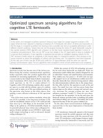
The block diagram of the algorithm is shown in Figure
8. A more detailed description is shown below:
1- The approximation and detail after every FWT
decomposition stage shall be denoted by the name
section. So, first of all, the power of each section is
computed.
2- Then the number of channels per section in this
stage is computed as (Total Number of LTE Chan-
nels)/2
(Decomposition Stage)
. and then used to get the
power per LTE channel.
3- It is assumed that there exists another location
awareness module not implemented here, this mod-
ule provides us with some important parameters
like:
A. Large-scale environmental parameters:
• Average LTE signal power, which depends on
the distance from the transmitter and the
Figure 4 LTE sensing algorithm flow chart.
Abdelmonem et al. EURASIP Journal on Wireless Communications and Networking 2012, 2012:6
/>Page 7 of 19
transmitted power. In case of femtocells, this
parameter will be different from the case of a
macro cell.

• Shadowing margin, which depends on the
environment whether it is urban, sub-urban, or a
rural area.
B. Small scale en vironmental parameters such as t he
fading margin that depends on the wireless channel
between the femtocell and the u ser, this parameter
also varies depending on whether we are considering
femto or macro cells.
C. Sensing parameters:
• Positive margin: Used to calculate the upper
threshold value above which the section is con-
sidered to be occupied.
• Negative margin: Used tocalculatethelower
threshold value below which the section is con-
sidered to be vacant, this value should be more
conservative than the positive threshold as it will
decide for this section and its channels to be
vacant.
Regarding the operation of the location awareness
module; we assume that this module has previous infor-
mation regarding the network paramet ers and especially
the cell transmission power; it can also determine the
location of t he user with respect to the cell using a cer-
tain determination mechanism (such as GPS). It can
also estimate the type of t he wireless channel over
which the user communicates using a certain channel
estimation techniques. Consequently, it can use a certain
look up table that maps the estimated channel para-
meters to the corresponding shadowing and fading mar-
gins. An example of the location awareness engine

0 5 10 15 20 25 30
0
0.02
0.04
0.06
0.08
0.1
0.12
0.14
0.16
0.18
Resource Block Index
|H(f)|
Figure 5 LTE channel spectrum with some RBs unoccupied in
the OFDM symbols other than 0 and 4 which do not have
pilots.
0 0.2 0.4 0.6 0.8
1
0
0.1
0.2
0.3
0.4
0.5
0.6
0.7
0.8
0.9
1
Pf

Pd
db2 FWT
db4 FWT
db10 FWT
512 point FFT
256 point FFT
128 point FFT
Figure 6 ROC for FWT versu s FFT based sensing in case of a 4 RB resolution sensing in an AWGN channel at -8 dB SNR and sensing
duration of 2.5 ms.
Abdelmonem et al. EURASIP Journal on Wireless Communications and Networking 2012, 2012:6
/>Page 8 of 19
architecture is shown in [31].
4- Then the upper and lower thresholds are com-
puted as follows:
• Upper threshold = Average power + Fading
margin + Positive sensing margin
• Lower threshold = Average power - Fading
margin - Negative sensing margin - Shadowing
margin
5- These thresholds are used to decide for the chan-
nel state:
• If Power > Upper threshold, the section state is
consid ered occupied, thus no further wavelet fil-
tering is applied as the LTE channels in this sec-
tion will be considered occupied.
• If Power < Lower threshold, the section state is
considered vacant thus no further wavelet filter-
ing is applied and the LTE channels in this sec-
tion will be considered vacant.
• Otherwise, the section state is considered nor-

mal so we shall continue applying wavelet filter-
ing as in the normal case.
&RPSXWH
6HFWLRQ
$SSUR[LPDWLRQ
3RZHU
&RPSXWH
6HFWLRQ'HWDLO
3RZHU
$SSUR[LPDWLRQ
'HWDLO
&RPSXWH1XPEHURI
&KDQQHOV6HFWLRQ
'HFRPSRVLWLRQ
6WDJH
1XPEHU2I
7UDQVPLWWHUV
&RPSXWH
$SSUR[LPDWLRQ
3RZHUSHU
&KDQQHO
&RPSXWH
'HWDLO
3RZHUSHU
&KDQQHO
/RFDWLRQDZDUHQHVV
PRGXOH
6HQVLQJ
SDUDPHWHUV
&RPSXWHXSSHUDQGORZHU

WKUHVKROGV
&RPSDUHZLWKWKH
8SSHUDQGORZHU
WKUHVKROGV
&RPSXWHWKH
ZHLJKWHGDYHUDJH
RIWKHFKDQQHO
VWDWHVDQGILOOWKH
VWDWHPDWUL[
/DUJHVFDOH
SDUDPHWHUV
6PDOOVFDOH
SDUDPHWHUV
Figure 8 Detailed block diagram for the ID algorithm using FWT.
,QSXW
6LJQDO
'$
'
$$ ''$'
'$'$$'
$
$'$ ''$ '''$''$$$ '$$
&KDQQHO2FFXSLHG
&KDQQHO9DFDQW
Figure 7 ID algorithm using FWT.
Abdelmonem et al. EURASIP Journal on Wireless Communications and Networking 2012, 2012:6
/>Page 9 of 19
6- The declared “state” is used to fill a “state matrix”
upon which we make our decision to apply wavelet
filtering or not as described above. The state matrix

has two dimensions: section and decomposition
stage a s shown in Figure 9. The section dimension
(horizontal) represents th e part of the LTE spectrum
being sensed, while t he decomposition stage dimen-
sion (vertical) represents the FWT current decompo-
sition stage.
The algorithm performance depends on the location
awareness module accuracy as well the wireless environ-
ment in which the sensing is done. In our simulations,
the following assumptions have been made:
- The channel is an AWGN channel thus the fading
and shadowing margins equal to zero.
- The average power received from the base station
is known.
The positive and negative sensing margins are cha n-
ged to span a range of upper and lower sensing thresh-
olds. These two thresholds control three main
performance metrics: probability of detection, prob abil-
ity of false alarm, and the average number of FWT
operations. When the differe nce between the upper and
lower sensing thresholds increases, the average number
of FWT operations increases as in this case the prob-
ability that the ID algorithm decides for a channel to be
vacant or occupied will decrease. At the same t ime, the
performance w ill be better than the case when the dif-
ference between the upper and lower sensing thresholds
is reduced. So, as shown in Fi gure 10, each curve repre-
sents a certain value for the difference between the
upper and lower sen sing thresholds, thus a certain value
for the average number of FWT operations. A trade off

has to be made between the performance (P
d
and P
f
)
and the computation al complexity (average number of
FWT operations) of the sensing algorithm. To conclude,
the number of decomposition levels is determined heur-
istically taking into consideration the following:
- The application using the algorithm and how much
sensitive it is to the sensing false alarm rate that
leads to some waste of bandwidth.
- The application of the primary user and how much
sensitive it is to a missed detection by the cognitive
user that consequently affects the primary user QOS.
- The hardware requirements and power consump-
tion requirements of the sensing module.
It also has to be taken into consideration that deciding
for the whole section to be vacant is a critical decision
as this means that all of its channels will be considered
vacant as well, thus the secondary use r can use them
after passing the fine sensing stage. That is why the
neg ative sensing threshold should be more conservative
than the positive one as it will affect the lower threshold
below which the section is considered vacant. This algo-
rithm shows a clear advantage of FWT over FFT as it
could not be applied on FFT.
The simulation results have shown that the perfor-
mance of the ID algorithm is quite close to the normal
algorithm in case of a regular pattern for LTE channel

occupancy(i.e.,11001100),whichmeanswe
achieve the same performance with reduced complexity
asshowninFigure11incaseofanAWGNchannel
and Figure 12 in case of multipath fading channels.
While in case of a random pattern the performance var-
ies as shown before in Figure 10.
A further enhancement to the ID algorithm is now i n
order. It is possible to compute a weighted average of
the channel states to take the final decision. This weight
is a function of the difference between the channel
power and the predefined threshold. In case the channel
power is far below or above the threshold, a higher
Figure 9 An example for the state matrix of the ID algorithm for a 3-stage FWT sensing.
Abdelmonem et al. EURASIP Journal on Wireless Communications and Networking 2012, 2012:6
/>Page 10 of 19
weight is given to the corresponding state whic h is
vacant or occupied, respectively.
Two different weights are defined:
- Confidence Metric Algorithm 1 uses the difference
between the channel power and the predefined
threshold,
-ConfidenceMetricAlgorithm2usesthesquareof
the difference between the channel power and the
predefined threshold.
Figure 13 shows the performance of the confidence
metric algorithm added to the ID algorithm. From the
0 0.1 0.2 0.3 0.4 0.
5
0.75
0.8

0.85
0.9
0.95
1
Pf
Pd
Without ID, 7 FWT Operations
With ID, 6.9 FWT Operations
With ID, 3.11 FWT Operations
Figure 11 ID algorithm performance versus the normal FWT algorithm for three decomposition stages in an AWGN channel at -5 dB
SNR and FWT sensing duration of 0.5 ms in case of a regular pattern for LTE channel occupancy.
0 0.2 0.4 0.6 0.8 1
0
0.1
0.2
0.3
0.4
0.5
0.6
0.7
0.8
0.9
1
Pf
Pd


Normal FWT (7 Operations)
Avg FWT Operations = 6.3
Avg FWT Operations = 6

Avg FWT Operations = 5.5
Avg FWT Operations = 4
Figure 10 ID algorithm performance versus the normal FWT algorithm for three decomposition stages in an AWGN channel at -5 dB
SNR and FWT sensing duration of 0.5 ms.
Abdelmonem et al. EURASIP Journal on Wireless Communications and Networking 2012, 2012:6
/>Page 11 of 19
figure, one can conclude the following:
-ForhigherP
d
, the confidence metric algorithm
gives better results. In case of spectrum sensing,
higher P
d
is more important than lower P
f
,asin
case of a missed detection this will lead to collision
with the primary user, which is unaccep table for CR
systems.
0 0.02 0.04 0.06 0.08 0.1 0.1
2
0.4
0.5
0.6
0.7
0.8
0.9
1
Pf
Pd

No Confidence Metric Alg
Confidence Metric Alg 1
Confidence Metric Alg 2
Figure 13 Confidence metric algorithm performance after being added to the original ID algorithm in an AWGN channel at -5 dB SNR
and FWT sensing duration of 0.5 ms in case of an irregular pattern for LTE channel occupancy.
0 0.05 0.1 0.15 0.
2
0.4
0.5
0.6
0.7
0.8
0.9
1
Pf
Pd
Without ID, 7 FWT Operations
With ID, 3.8 FWT Operations
With ID, 5.5 FWT Operations
With ID, 5.7 FWT Operations
Figure 12 ID algorithm performance versus the normal FWT algorithm for three decomposition stages in an EPA channel, 5 Hz
Doppler at -5 dB SNR and FWT sensing duration of 0.5 ms in case of a regular pattern for LTE channel occupancy.
Abdelmonem et al. EURASIP Journal on Wireless Communications and Networking 2012, 2012:6
/>Page 12 of 19
- In case of l ower probability of false alarm, using
confidence metric algorithm gives a worse perfor-
mance than the normal algorithm. This observation
may vary according to the values of the chosen

thresholds. In case we choose different threshold
values, we could end up with the algorithm being
better in case of lower probability of false alarm.
The optimal calculation of the thresholds is out of
scope of this study and co uld be added in the fu ture
study.
- In general, using algorithm 1 is better than algo-
rithm 2 where using the square of the differen ce
enlarges the large differences and reduces the small
differences, which might lead to false decisions as
compared to using the difference alone without
squaring.
After discussing the optimizations done to the FWT
algorithm in order to reduce the algorithm complexity
and after comparing FWT versus FFT in terms of the
number of computations done in each operation for a
given performance in Section 2.2, we can now have a
more global view in Table 3 regarding when we should
use FWT for the coarse sensing stage and when to use
it from a practical perspective as well.
3. LTE fine spectrum sensing
Referring to the main system flow chart in Figure 4, we
have shown that the coarse sensing module mainly con-
centrates on quick detectio n of empty spaces to be used
by the CR user. But in order to have a more reliable
detection for t he empty spaces, we need to perform fine
sensing on them. In this section, two fine sensing algo-
rithms are propo sed; one of them uses the cyclic shift
property of the LTE OFDM signal while the other one
uses one of the LTE synchronization signals. A detailed

explanation is given for the two proposed fine sensing
algorithms along with their results and en hancements.
Finally, the end-to-en d system results are shown in case
of different coarse and fine sensing module pairs.
3.1 Cyclic prefix correlation sensing
3.1.1 Normal CP algorithm
In this algorithm, CP correlation usin g a sliding window
is performed over a number o f OFDM symbols. The
peak indices are the n investigated and the decision for
LTE signal existence is based on a majority vote for the
number of peaks. The normal cyclic prefix configuration
is assumed where the first OFDM symbol in the slot has
a CP composed of 160 samples compared to 144 sam-
ples for the remaining 6 OFDM symbols.
Assuming the following:
- Input signal is X(n)
- The correlator output is Y(n)
- The correlation window size is 160 which is the
maximum CP length. The FFT size is denoted by
the symbol N
FFT
. It is important to note here that if
the window size is taken to be 144, the algorithm
will be suboptimum in case of the first OFDM sym-
bol in the slot because the first symbol has a CP of
length 160 samples, while f or the other symbols, the
CP length is 144 samples. In that case, we are not
making use of the whole 160 samples in the CP of
this symbol. For the remaining symbols, the correla-
tion will be optimum in case of a 144 length window

because we sha ll use the whole 14 4 CP samples in
the correlation.
The CP correlation is as follows:
Y(sample) =
n=Window Size

n=1
X(sample + n) × X
∗
(sample + n + NFFT)
(3)
Every tick (time sample), the sliding window is shifted
by one sample and the new correlator out put is com-
puted. The peaks of th e correlator output are comp ared
against a predefined threshol d after which a decision is
made whether an LTE signal is present or not. From an
implementation point of view, the above algorithm
could be further simplified as follows: instead of per-
forming 160 multiplications and additions for each
Table 3 A global comparison between FWT and FFT coarse sensing methods
FWT FFT
Better at obtaining a higher P
d
which is important to satisfy the required
primary user QoS. Used when the primary user QoS is of higher concern
Better at obtaining a lower P
f
which is important to achieve better
spectral efficiency. Used when the spectral efficiency is of higher
concern

The sensing resolution could be simply increased to reach RB resolution
by applying further FWT decompositions
To increase the sensing resolution we need to increase the FFT size
An ID algorithm could be applied at each wavelet decomposition stage
to reduce the number of FWT operations with an acceptable
performance
The ID algorithm is not applicable to FFT where the operation is
performed in one stage
In case the LTE receiver is an SDR and has a programmable FFT core, we
lose the option of reusing this core which is used in the LTE OFDM
receiver to perform spectrum sensing
When the receiver is an SDR with a programmable FFT core, we can
simply reuse the same FFT core used in the LTE OFDM receiver to
perform spectrum sensing thus reducing complexity
Abdelmonem et al. EURASIP Journal on Wireless Communications and Networking 2012, 2012:6
/>Page 13 of 19
correlator o utput, one can simply add one sample and
subtract one sample using an iterative equation. In this
case, we have only two additions and multiplications per
output sample excluding the first correlator output sam-
ple. In other words, in case of the first output sample
(sample = 0), the correlator output is given by:
Y(0) =
n=Window Size

n=1
X(n) × X
∗
(n + NFFT)
(4)

0 0.2 0.4 0.6 0.8 1
0
0.1
0.2
0.3
0.4
0.5
0.6
0.7
0.8
0.9
1
Pf
Pd


ETU 70Hz -5dB
ETU 300Hz -5dB
EPA 5Hz -10dB
EVA 5Hz -8dB
EVA 30Hz -8dB
Figure 14 ROC for CP correlation sensing in different wireless LTE channel models.
0 0.2 0.4 0.6 0.8 1
0
0.1
0.2
0.3
0.4
0.5
0.6

0.7
0.8
0.9
1
Pf
Pd
CP correlation with Folding, ETU 70 Hz -8 dB
CP correlation without Folding, ETU 70 Hz -8 dB
Figure 15 ROC for CP correlation with folding versus without folding in an ETU channel at -8 dB SNR with 70 Hz Doppler frequency.
Abdelmonem et al. EURASIP Journal on Wireless Communications and Networking 2012, 2012:6
/>Page 14 of 19
While in case of the other samples greater than zero:
Y(sample) = Y(sample − 1) + X(sample + Window Size)
× X
∗
(sample + Window Size + NFFT)
− X(sample − 1) × X
∗
(sample − 1+NFFT)
(5)
In our simulations, the second approach is used due
to its reduced complexity. In Figure 14, the ROC is
shown for CP correlation sensing. The algorithm was
tested in case of the following LTE channel models:
Extended Ty pical Urban (ETU), Extended Vehicular A-
model, and Extended Pedestrian A-model (EPA) at dif-
ferent noise levels.
3.1.2 CP algorithm with folding
In this algorithm, we use the same CP correlation
method but instead of inserting the correlator resul ts in

a buffer equal to the i nput signal length, the buffer size
this time is chosen to be equal to N
FFT
+ correlation
window size. The correlation output for the current
symbol is folded with that of the previo us symbol and
so on. The input-output relation will be as follows:
Y(output sample) =
n=Correlation Window Size

n=1
X(input sample + n) × X
∗
(input sample + n + NFFT)
(6)
where
output sample = mod
(
input sample, correlation buffer size
)
(7)
correlation buffer size = NFFT + correlation window size
(8)
Figure 15 compares the performance of the two CP
correlation algorithms. Thefigureshowsanobvious
improvement for using the folding algorithm against
without f olding especially in multipath fading channels
like the ETU channel. In addition to the better perfor-
mance, this algorithm requires a smaller correlation buf-
fer size which means lower hardware complexity as well.

3.2 Primary sync correlation sensing
In LTE, there are three known signals transmitted in the
downlink: the Primary synchronization signal (P-SCH),
the Secondary synchronization signal (S-SCH), and the
reference signals (Pilots). Our main target in this section
is to design an algorithm that detects the LTE signal
reliably and with the l east possible complexity using the
above mentioned known signals. We can simply corre-
late the received signal with a replica from the synchro-
nization signals and compare the correlation peak
against a certain threshold to indicate the existence of
an LTE signal. The question now is which one of the
above three signals could be used. As for the P-SCH,
although it is generated as an OFDM signal, it could be
entirely detected in the time-domain with no need for
an FFT operation. The S-SCH, however, is typically
detected in the frequency domain. Moreover, in LTE,
there are 504 cell IDs which are divided into 168 group
IDs, where each group contains three identities. The
168 groups are encoded into the S-SCH whereas the P-
SCH signal index determines the identity within the
group [32].
It is clear from the above that using P-SCH is m uch
simpler than the S-SCH for two reasons:
1- Only three correlations need to be carried out
instead of 168 correlations if S-SCH is used.
2- Detection could be performed in the time domain
with no need for FFT processing before correlation.
Using the LTE Referenc e signals (pilots) for fine sen-
sing will be very difficult as it requires the knowledge of

the slot and symbol index in addition to the w hole cell
ID.ThatiswhytheP-SCHischosentoperformthe
fine sensing algorithm for LTE.
In LTE, several bandwidths (up to 20 MHz) are sup-
ported and the minimum system bandwidth (1.25 MHz)
corresponds to six RBs. With 15 kHz subca rrier spacing,
the synchronization signal may occupy at most 72 sub-
carriers to comply with the minimum bandwidth in the
LTE bandwidth sets. It would typically be generated by
a 128-point FFT. However, to allow matched filter
impl ementations with lengths shorter than 128 samples,
the P-SCH signals are defined as OFDM signals with up
to 64 subcarriers, including the DC subcarrier. Such a
signal can be detected by a matched filter of length 64.
In the frequency domain of the P -SCH, 62 active sub-
carriers are used, centered around the null DC subcar-
rier as follows:
d
u
(
n
)
=
⎧
⎪
⎪
⎨
⎪
⎪
⎩

e
−j
∂un
(
n +1
)
63
, n = 0, 1, 2, ,30
e
−j
∂u
(
n +1
)(
n +2
)
63
, n = 31, 32, , 61
(9)
Numerous investigations were done in 3GPP for the
selection of the sequence indices u. It was concluded
that the sensitivity to large frequency offsets was smal-
lest when the indices are selected close to half the
sequence length. The sequence indices have been cho-
sen as u = 25, 29, and 34. Also it can easily be proved
that the signal obtained from u = 29 is a complex conju-
gated version of u = 34, this property will lead to a
reduction in the matched filt er complexity as the two
corresponding matched filters can be implemented with
the multiplication complexity of just one filter as shown

below:
Assume that the received signal ‘r’ shall be correlated
with a locally generated replica of the P-SCH ‘s’
r × s =Re{r}×Re {s}−Im {r}×Im {s} + j
(
Re {r}×Im {s}×Re {s}
)
(10)
Abdelmonem et al. EURASIP Journal on Wireless Communications and Networking 2012, 2012:6
/>Page 15 of 19
r × s∗ =Re{r}×Re {s} +Im{r}×Im {s} + j
(
Im {r}×Re {s}−Re {r}×Im {s}
)
(11)
We can see from the above equations [33] that the
difference lies only in the signs and that we can perform
the multiplications only once. The P-SCH signal is also
centrally symmetric, which me ans that the number of
multiplications in the corresponding matched filter
could be reduced. There are 62 centrally symmetric
samples of the P-SCH signal. These sample pairs can be
added prior to multiplication, so the matched filter can
be implemented by almost half the multiplications
required in the direct implementation.
0 0.05 0.1 0.15 0.
2
0.6
0.65
0.7

0.75
0.8
0.85
0.9
0.95
1
Pf
Pd


ETU 70Hz -15dB
ETU 300Hz -15dB
EPA 5Hz -20dB
EVA 5Hz -20dB
EVA 30Hz -8dB
Figure 16 ROC of the P-SCH correlation algorithm in different LTE channel models.
0 0.2 0.4 0.6 0.8 1
0
0.1
0.2
0.3
0.4
0.5
0.6
0.7
0.8
0.9
1
Pf
a

Pd


ETU 300Hz -5dB CP Sensing (0.5msec)
ETU 300Hz -15dB Prim Sync Sensing (10msec)
Figure 17 ROC of the P-SCH correlation algorithm versus CP correlation sensing in an ETU channel.
Abdelmonem et al. EURASIP Journal on Wireless Communications and Networking 2012, 2012:6
/>Page 16 of 19
To conclude, complexity reduction is done in two
ways:
1- Minimizing the number of multiplications by half
for each matched filter through addition of sym-
metric samples.
2- Making it possible to det ect the three P-SCH sig-
nals with a multiplication complexity corresponding
to only two matched filters.
Figure 16 shows the performance of the P-SCH corre-
lation algorithm in different LTE channel models. Also
Figure 17 compares the performance of the P-SCH cor-
relation algorithm against CP correlation. Regarding the
performance of the P-SCH correlation sensing algorithm
in multipath fading channels, the simulation results
show that the algorithm is quite immune against delay
spread, Doppler spread and noise. I t also outperforms
the CP correlation algorithm even when the P-SCH
algorithm is operati ng at an SNR lower than that of the
CP algorithm. However, it is important to note that the
sensingdurationis10mswheretheP-SCHsignalsare
5 ms apart. On the other hand, although the perfor-
mance of the CP correla tion algorithm is not as good as

P-SCH sensing, the sensing duration could be reduced
to as low as 0.5 ms. So, there exists a compromise
between the sensing performance and sensing duration.
Increasing the sensing duration of t he CP correlation
sensing algorithm to 10 ms is not practical as this will
mean performing too many unnecessary CP correlations
(Number of OFDM symbols per slot (7) × number of
slots (20) = 140 CP correlations), w hile in case of P-
SCH sensing, we have only two P-SCH signals in a 10
ms duration.
3.3 End-to-end system results
In this section, we show some results of the proposed
end-to-end LTE spectrum sensing architecture proposed
including both the coarse and fine sensing modules col-
lectively. Figure 18 compares between using an FFT
coarse sensing module alone versus using the fine CP
correlation sensing after the coarse sensing. It is quite
clear that the fine sensing module has improved the
spectrum sensing performance. It also shows the gain of
using the P-SCH correlation fine sensing module after
the coarse FWT sensing module versus using the coarse
sensing module alone in an AWGN channel. Finally Fig-
ure 19 shows the performance of the FWT and P-SCH
correlation modules collectively in case of multipath fad-
ing LTE channel models.
4. Conclusions
In this article, spectrum sensing is performed for an
LTE signal in two stages; a coarse stage and a fine stage.
Analgorithmisproposedthatusesthewaveletpacket
transform algorithm to perform the coarse sensing stage

0 0.2 0.4 0.6 0.8 1
0
0.1
0.2
0.3
0.4
0.5
0.6
0.7
0.8
0.9
1
Pf
Pd
FWT alone
FWT + P-SCH Correlation
FFT + Fine CP correlation
FFT alone
Figure 18 A graph showing the effect of FFT coarse sensing module alone versus using the fine CP correlation sensing after the
coarse sensing for a 2.5 m sensing duration. FWT coarse sensing module is also investigated alone versus using the fine P-SCH correlation
sensing after the coarse sensing for a 10-ms sensing duration. Both simulations are done in an AWGN channel, -5 dB SNR.
Abdelmonem et al. EURASIP Journal on Wireless Communications and Networking 2012, 2012:6
/>Page 17 of 19
assuming that the primary signal is an LTE signal. The
challenges associated with the pro posed algorithm are
mentioned as well as a comparison with FFT-based
coarse detection in terms of both performance and com-
plexity has been introduced. The comparison shows that
FWT and FFT have almost the same performance.
Simulations have shown that reducing the sensin g reso-

lution of the FWT algorithm to an RB requires sharp fil-
ters and is impractical, that is why sensing is done at
multiples of an RB. Also, a new ID algorithm has led to
a further reduction in the FWT complexity where we
provide a stop ping criterion for t he normal FWT algo-
rithm based on en vironmental parameters and pre-
defined thresholds, this provides FWT sensing with an
advantage over FFT sensing as the algorithm is not
applicable to FFT. The results of this algorithm have
shown t hat a compromise has to be made b etween the
FWT complexity and the required probability of detec-
tion and false alarm. Optimally setting the thresholds of
this algorithm is a subject of future research. A confi-
dence metric has b een added to the ID algorith m which
mainly applies a weighted average of the sensed channel
states to arrive at the final decision. This weight i s a
function of the difference b etween the chann el power
and the predefined threshold. The confidence metric
algorithm outperforms the normal one in case high P
d
is required, which is the most important parameter in
case of spectrum sensing for CR systems.
In the fine sensing stage, two algorithms are proposed.
The first algorithm is the CP correlation sensing. An
iterative structure with fewer multiplications is com-
pared versus the normal structure in terms of compl ex-
ity where both algorithms provide the same
performance. Also, simulat ions results have shown that
using folding in CP correlation reduces the correlation
buffer size and increases the sensing gain especially in

multipath channels. The sec ond proposed fine sensing
algorithm requires one of the know n LTE synchroniza-
tion signals, we have shown that using the P-SCH is the
most suitable as the S-SCH and p ilots require far more
complexity. The P-SCH correlation algorithm was
proved to be more reliable than the CP correlation algo-
rithms in different LTE channel models. Finally, the
end-to-end system results show the gain obtained in
case of using the fine sensing module after the coarse
oneversususingthecoarsemodulealonefordifferent
coarse and fine module pairs.
Acknowledgements
This article has been presented in part at the 17th IEEE International
Conference on Telecommunications (ICT) 2010, Doha, Qatar, April 2010.
Competing interests
The authors declare that they have no competing interest s.
Received: 20 July 2011 Accepted: 9 January 2012
Published: 9 January 2012
0 0.2 0.4 0.6 0.8 1
0
0.1
0.2
0.3
0.4
0.5
0.6
0.7
0.8
0.9
1

Pf
Pd
FWT + P-SCH, EPA 5 Hz -5 dB
FWT + P-SCH, EVA 70 Hz -5 dB
FWT + P-SCH, ETU 300 Hz -5 dB
Figure 19 ROC of FWT coarse sensing with fine P-SCH correlation sensing in different wireless LTE channel models, 10-ms sensing
duration.
Abdelmonem et al. EURASIP Journal on Wireless Communications and Networking 2012, 2012:6
/>Page 18 of 19
References
1. Federal Communications Commission, Spectrum Policy Task force Report,
ET Docket No. 02-135. (November 2002)
2. S Haykin, Cognitive radio: brain-empowered wireless communications. IEEE
J Sel Areas Commun. 23(2), 201– 220 (2005)
3. J Mitola III, GQ Maguire Jr, Cognitive radio: making software radios more
personal. IEEE Personal Commun. 6,13–18 (1999). doi:10.1109/98.788210
4. J Mitola III, Cognitive radio for flexible mobile multimedia communications.
Mob Netw Appl. 6, 435–441 (2001). doi:10.1023/A:1011426600077
5. E Dahlman, S Parkvall, J Sköld, P Beming, 3G Evolution HSPA and LTE for
Mobile Broadband, 1st edn. (Academic Press, Oxford, 2007)
6. L Wang, Y Zhang, Z Wei, Mobility management schemes at radio network
layer for LTE femtocells, in Proceedings of IEEE Vehicular Technology
Conference, Barcelona, pp. 1–5 (2009)
7. R Rakken, Femtocells for Wireless in the Home and Office, Femto Forum
(2010)
8. R Agumamidi, Concept and Challenges of Femtocells, Project Report,
Department of EE, Pennsylvania State University (2010)
9. V Chandrasekhar, JG Andrews, Uplink capacity and interference avoidance
for two-tier cellular networks, in IEEE, GLOBECOM 2007, Washington, DC, pp.
3498–3509 (2007)

10. D López-Pérez, A Valcarce, G de la Roche, J Zhang, OFDMA femtocells: a
roadmap on interference avoidance. IEEE Commun Mag. 47,41–48 (2009)
11. ME Sahin, I Guvenc, M Jeong, H Arslan, Handling CCI and ICI in OFDMA
femtocell networks through frequency scheduling. IEEE Trans Consum
Electron. 55, 1936–1944 (2009)
12. P Kulkarni, W Hau Chin, T Farnham, Radio resource management
considerations for LTE femto cells. ACM SIGCOMM Comput Commun
Rev.40(1), 26–30
13. H Claussen, Performance of macro and co-channel femtocells in a
hierarchical cell structure, in IEEE PIMRC 2007, Athens, Greece, pp. 1–5 (2007)
14. Y Li, Cognitive interference management in 4G autonomous femtocells,
PhD Thesis, (University of Toronto, ECE Department, 2010)
15. J Lotze, SA Fahmy, B Ozgul, J Noguera, LE Doyle, Spectrum sensing on LTE
femtocells for GSM spectrum re-farming using Xilinx FPGA. SDR Forum, SDR
Technical Conference and Product Exposition, Washington, DC (2009)
16. Draft Standard for Wireless Regional Area Networks Part 22, Cognitive
Wireless RAN Medium Access Control (MAC) and Physical Layer (PHY)
specifications: Policies and procedures for operation in the TV Bands. IEEE
P802.22™/D0.4.4
17. T Yucek, H Arslan, A survey of spectrum sensing algorithms for cognitive
radio applications. IEEE Commun Surv Tutor. 11(1), 116–130 (2009)
18. Y Youn, H Jeon, J Hwan Choi, H Lee, Fast spectrum sensing algorithm for
802.22 WRAN systems, in IEEE ISCIT 2006, Thailand, pp. 960–964 (2006)
19. T Yucek, H Arslan, Spectrum characterization for opportunistic cognitive
radio systems, in IEEE Military Communications Conference 2006, Washington,
DC, USA, pp. 1–6 (2006)
20. N Khambekar, L Dong, V Chaudhary, Utilizing OFDM guard interval for
spectrum sensing, in IEEE Wireless Communications and Networking 2007,
Hong Kong, pp. 38–42 (2007)
21. K Kim, IA Akbar, KK Bae, J-S Um, CM Spooner, JH Reed, Cyclostationary

approaches to signal detection and classification, in IEEE International
Symposium on New Frontiers in Dynamic Spectrum Access Networks 2007,
Dublin, Ireland, pp. 212–215 (2007)
22. S Tu, K Chen, R Prasad, Spectrum Sensing of OFDMA systems for cognitive
radios, in The 18th annual IEEE International Symposium on Personal, Indoor
and Mobile Radio Communications (PIMRC’07), Athens, Greece, pp.
3410–3425 (2007)
23. H Chen, W Gao, DG Daut, Signature based spectrum sensing algorithms for
IEEE 802.22 WRAN, in IEEE Comm Society ICC 2007, Glasgow, Scotland, pp.
6487–6492 (June 2007)
24. A Ghasemi, ES Sousa, Spectrum sensing in cognitive radio networks:
requirements, challenges and design trade-offs. IEEE Commun Mag. 46,
32–39 (2008)
25. E Peh, Y Liang, Optimization for cooperative sensing in cognitive radio
networks, in IEEE, WCNC 2007, Hong Kong, pp. 3411–3415 (2007)
26. H Arslan, in Cognitive Radio, Software Defined Radio, and Adaptive Wireless
Systems, (Springer, New York, 2007)
27. H Tang, Some physical layer issues of wide-band cognitive radio, in IEEE
International Symposium on New Frontiers in Dynamic Spectrum Access
Networks 2005, Baltimore, MD, USA, pp. 151–159 (2005)
28. AF Cattoni, I Minetti, M Gandetto, R Niu, PK Varshney, CS Regazzoni, A
spectrum sensing algorithm based on distributed cognitive models, in SDR
Forum Technical Conference, Orlando, FL, USA, pp. 1–6 (2006)
29. 3GPP, E-UTRA Physical Channels and Modulation, (Release 8). (2008)
30. RC Gonzalez, RE Woods, in Digital Image Processing, vol. Ch. 7, 2nd edn.
(Prentice-Hall, Upper Saddle River, NJ, 2002)
31. H Celebi, H Arslan, Utilization of location information in cognitive wireless
networks. IEEE Wirel Commun Mag. 14,6–13 (2007)
32. K Manolakis, D Estevez, V Jungnickel, W Xu, A closed concept for
synchronization and cell search in 3GPP LTE systems, in IEEE, WCNC 2009,

Hungary, pp. 1–6 (2009)
33. BM Popovic, F Berggren, Primary synchronization signal in E-UTRA, in IEEE
International Symposium on Spread Spectrum Techniques and Applications,
Bologna, Italy, pp. 426–430 (2008)
doi:10.1186/1687-1499-2012-6
Cite this article as: Abdelmonem et al.: Optimized spectrum sensing
algorithms for cognitive LTE femtocells. EURASIP Journal on Wireless
Communications and Networking 2012 2012:6.
Submit your manuscript to a
journal and benefi t from:
7 Convenient online submission
7 Rigorous peer review
7 Immediate publication on acceptance
7 Open access: articles freely available online
7 High visibility within the fi eld
7 Retaining the copyright to your article
Submit your next manuscript at 7 springeropen.com
Abdelmonem et al. EURASIP Journal on Wireless Communications and Networking 2012, 2012:6
/>Page 19 of 19