Báo cáo toán học: " Minimal and maximal solutions to first-order differential equations with state-dependent deviated arguments" pptx

This Provisional PDF corresponds to the article as it appeared upon acceptance. Fully formatted
PDF and full text (HTML) versions will be made available soon.
Minimal and maximal solutions to first-order differential equations with
state-dependent deviated arguments
Boundary Value Problems 2012, 2012:7 doi:10.1186/1687-2770-2012-7
Ruben Figueroa ()
Rodrigo Lopez Pouso ()
ISSN 1687-2770
Article type Research
Submission date 13 May 2011
Acceptance date 20 January 2012
Publication date 20 January 2012
Article URL />This peer-reviewed article was published immediately upon acceptance. It can be downloaded,
printed and distributed freely for any purposes (see copyright notice below).
For information about publishing your research in Boundary Value Problems go to
/>For information about other SpringerOpen publications go to

Boundary Value Problems
© 2012 Figueroa and Lopez Pouso ; licensee Springer.
This is an open access article distributed under the terms of the Creative Commons Attribution License ( />which permits unrestricted use, distribution, and reproduction in any medium, provided the original work is properly cited.
Boundary Value Problems manuscript No.
(will be inserted by the editor)
Minimal and maximal solutions to first-order
differential equations with state-dependent
deviated arguments
Rub´en Figueroa
∗
and Rodrigo L´opez Pouso
Department of Mathematical Analysis, University of Santiago de Compostela,
Spain
∗

Corresp onding author: ruben.fi
E-mail address:
RLP:
Abstract
We prove some new results on existence of solutions to first-order ordinary
differential equations with deviated arguments. Delay differential equations
are included in our general framework, which even allows deviations to de-
pend on the unknown solutions. Our existence results lean on new definitions
of lower and upper solutions introduced in this article, and we show with an
example that similar results with the classical definitions are false. We also
introduce an example showing that the problems considered need not have
the least (or the greatest) solution between given lower and upper solutions,
2 Rub´en Figueroa
∗
and Rodrigo L´opez Pouso
but we can prove that they do have minimal and maximal solutions in the
usual set–theoretic sense. Sufficient conditions for the existence of lower and
upper solutions, with some examples of application, are provided too.
1 Introduction
Let I
0
= [t
0
, t
0
+ L] be a closed interval, r ≥ 0, and put I
−
= [t
0
− r, t

0
] and
I = I
−
∪ I
0
. In this article, we are concerned with the existence of solutions
for the following problem with deviated arguments:







x

(t) = f (t, x(t), x(τ(t, x))) for almost all (a.a.) t ∈ I
0
,
x(t) = Λ(x) + k(t) for all t ∈ I
−
,
(1)
where f : I × R
2
−→ R and τ : I
0
× C(I) −→ I are Carath´eodory functions,
Λ : C(I) −→ R is a continuous nonlinear operator and k ∈ C(I

−
). Here C(J)
denotes the set of real functions which are continuous on the interval J.
For example, our framework admits deviated arguments of the form
τ(t, x) = sin
2
(x(t)) t
0
+ (1 − sin
2
(x(t))) (t
0
+ L),
or
τ(t, x) = t −

I
|x(s)| ds
1 +

I
|x(s)| ds
r.
We define a solution of problem (1) to be a function x ∈ C(I) such that
x
|I
0
∈ AC(I
0
) (i.e., x

|I
0
is absolutely continuous on I
0
) and x fulfills (1).
In the space C(I) we consider the usual pointwise partial ordering, i.e.,
for γ
1
, γ
2
∈ C(I) we define γ
1
≤ γ
2
if and only if γ
1
(t) ≤ γ
2
(t) for all t ∈ I.
A solution of (1), x
∗
, is a minimal (respectively, maximal) solution of (1) in
Title Suppressed Due to Excessive Length 3
a certain subset Y ⊂ C(I) if x
∗
∈ Y and the inequality x ≤ x
∗
(respectively,
x ≥ x
∗

) implies x = x
∗
whenever x is a solution to (1) and x ∈ Y . We say
that x
∗
is the least (respectively, the greatest) solution of (1) in Y if x
∗
≤ x
(respectively, x
∗
≥ x) for any other solution x ∈ Y . Notice that the least
solution in a subset Y is a minimal solution in Y , but the converse is false in
general, and an analgous remark is true for maximal and greatest solutions.
Interestingly, we will show that problem (1) may have minimal (ma-
ximal) solutions between given lower and upper solutions and not have
the least (greatest) solution. This seems to be a peculiar feature of equa-
tions with deviated arguments, see [1] for an example with a second-order
equation. Therefore, we are obliged to distinguish between the concepts
of minimal solution and least solution (or maximal and greatest solutions),
unfortunately often identified in the literature on lower and upper solutions.
First-order differential equations with state-dependent deviated argu-
ments have received a lot of attention in the last years. We can cite the
recent articles [2–7] which deal with existence results for this kind of prob-
lems. For the qualitative study of this type of problems we can cite the
survey of Hartung et al. [8] and references therein.
As main improvements in this article with regard to previous works in
the literature we can cite the following:
(1) The deviating argument τ depends at each moment t on the global
behavior of the solution, and not only on the values that it takes at the
instant t.

4 Rub´en Figueroa
∗
and Rodrigo L´opez Pouso
(2) Delay problems, which correspond to differential equations of the form
x

(t) = f(t, x(t), x(t − r)) along with a functional start condition, are
included in the framework of problem (1). This is not allowed in articles
[3–6].
(3) No monotonicity conditions are required for the functions f and τ, and
they need not be continuous with respect to their first variable.
This article is organized as follows. In Section 2, we state and prove
the main results in this article, which are two existence results for problem
(1) between given lower and upper solutions. The first result ensures the
existence of maximal and minimal solutions, and the second one establishes
the existence of the greatest and the least solutions in a particular case. The
concepts of lower and upper solutions introduced in Section 2 are new, and
we show with an example that our existence results are false if we consider
lower and upper solutions in the usual sense. We also show with an example
that our problems need not have the least or the greatest solution between
given lower and upper solutions. In Section 3, we prove some results on the
existence of lower and upper solutions with some examples of application.
2 Main results
We begin this section by introducing adequate new definitions of lower and
upper solutions for problem (1).
Title Suppressed Due to Excessive Length 5
Notice first that τ(t, γ) ∈ I = I
−
∪ I
0

for all (t, γ) ∈ I
0
× C(I), so for
each t ∈ I
0
we can define
τ
∗
(t) = inf
γ∈C(I)
τ(t, γ) ∈ I, τ
∗
(t) = sup
γ∈C(I)
τ(t, γ) ∈ I.
Definition 1 We say that α, β ∈ C(I), with α ≤ β on I, are a lower and
an upper solution for problem (1) if α
|I
0
, β
|I
0
∈ AC(I
0
) and the following
inequalities hold:
α

(t) ≤ min
ξ∈E(t)

f(t, α(t), ξ) for a.a. t ∈ I
0
, α ≤ inf
γ∈[α,β]
Λ(γ) + k on I
−
,(2)
β

(t) ≥ max
ξ∈E(t)
f(t, β(t), ξ) for a.a. t ∈ I
0
, β ≥ sup
γ∈[α,β]
Λ(γ) + k on I
−
,(3)
where
E(t) =

min
s∈[τ
∗
(t),τ
∗
(t)]
α(s), max
s∈[τ
∗

(t),τ
∗
(t)]
β(s)

(t ∈ I
0
),
and [α, β] = {γ ∈ C(I) : α ≤ γ ≤ β}.
Remark 1 Definition 1 requires implicitly that Λ be bounded in [α, β].
On the other hand, the values
min
ξ∈E(t)
f(t, α(t), ξ) and max
ξ∈E(t)
f(t, β(t), ξ),
are really attained for almost every fixed t ∈ I
0
thanks to the continuity of
f(t, α(t), ·) and f(t, β(t), ·) on the compact set E(t).
Now we introduce the main result of this article.
Theorem 1 Assume that the following conditions hold:
(H
1
) (Lower and upper solutions) There exist α, β ∈ C(I), with α ≤ β on I,
which are a lower and an upper solution for problem (1).
6 Rub´en Figueroa
∗
and Rodrigo L´opez Pouso
(H

2
) (Carath´eodory conditions)
(H
2
) − (a) For all x, y ∈ [min
t∈I
α(t), max
t∈I
β(t)] the function
f(·, x, y) is measurable and for a.a. t ∈ I
0
, all x ∈ [α(t), β(t)] and all
y ∈ E(t) (as defined in Definition 1) the functions f (t, ·, y) and f(t, x, ·)
are continuous.
(H
2
) − (b) For all γ ∈ [α, β] = {ξ ∈ C(I) : α ≤ ξ ≤ β} the function
τ(·, γ) is measurable and for a.a. t ∈ I
0
the operator τ(t, ·) is continuous
in C(I) (equipped with it usual topology of uniform convergence).
(H
2
) − (c) The nonlinear operator Λ : C(I) −→ R is continuous.
(H
3
) (L
1
−bound) There exists ψ ∈ L
1

(I
0
) such that for a.a. t ∈ I
0
, all x ∈
[α(t), β(t)] and al l y ∈ E ( t) we have
|f(t, x, y)| ≤ ψ(t).
Then problem (1) has maximal and minimal solutions in [α, β].
Proof. As usual, we consider the function
p(t, x) =















α(t), if x < α(t),
x, if α (t) ≤ x ≤ β(t),
β(t), if x > β(t),
and the modified problem








x

(t) = f (t, p(t, x(t)), p(τ (t, x), x(τ(t, x)))) for a.a. t ∈ I
0
,
x(t) = Λ(p(·, x(·))) + k(t) for all t ∈ I
−
.
(4)
Title Suppressed Due to Excessive Length 7
Claim 1: Problem (4) has a nonempty and compact set of solutions. Consider
the operator T : C(I) −→ C(I) which maps each γ ∈ C(I) to a continuous
function T γ defined for each t ∈ I
−
as
T γ(t) = Λ(p(·, γ(·))) + k(t),
and for each t ∈ I
0
as
T γ(t) = Λ(p(·, γ(·))) + k(t
0
) +

t

t
0
f(s, p(t, γ(s)), p(τ (s, γ), γ(τ(s, γ))))ds.
It is an elementary matter to check that T is a completely continuous opera-
tor from C(I) into itself (one has to take Remark 1 into account). Therefore,
Schauder’s Theorem ensures that T has a nonempty and compact set of fixed
points in C(I), which are exactly the solutions of problem (4).
Claim 2: Every solution x of (4) satisfies α ≤ x ≤ β on I and, therefore, it
is a solution of (1) in [α, β]. First, notice that if x is a solution of (4) then
p(·, x(·)) ∈ [α, β]. Hence the definition of lower solution implies that for all
t ∈ I
−
we have
α(t) ≤ Λ(p(·, x(·))) + k(t) = x(t).
Assume now, reasoning by contradiction, that x  α on I
0
. Then we can
find
ˆ
t
0
∈ [t
0
, t
0
+ L) and ε > 0 such that α(
ˆ
t
0
) = x(

ˆ
t
0
) and
α(t) > x(t) for all t ∈ [
ˆ
t
0
,
ˆ
t
0
+ ε]. (5)
Therefore, for all t ∈ [
ˆ
t
0
,
ˆ
t
0
+ ε] we have p(t, x(t)) = α(t) and
p(τ(t, x), x(τ (t, x))) ∈ [α(τ (t, x)), β(τ(t, x))] ⊂ E(t),
8 Rub´en Figueroa
∗
and Rodrigo L´opez Pouso
so for a.a. s ∈ [
ˆ
t
0

,
ˆ
t
0
+ ε] we have
α

(s) ≤ f (s, p(s, x(s)), p(τ (s, x), x(τ(s, x)))).
Hence for t ∈ [
ˆ
t
0
,
ˆ
t
0
+ ε] we have
α(t) − x(t) =

t
ˆ
t
0
α

(s) ds −

t
ˆ
t

0
f(s, p(s, x(s)), p(τ(s, x), x(τ (s, x)))) ds ≤ 0,
a contradiction with (5).
Similar arguments prove that all solutions x of (4) obey x ≤ β on I.
Claim
3
: The set of solutions of problem (1) in
[
α, β
]
has maximal and
minimal elements. The set
S = {x ∈ C(I) : x is a solution of (1) , x ∈ [α, β]}
is nonempty and compact in C(I), beacuse it coincides with the set of fixed
points of the operator T. Then, the real-valued continuous mapping
x ∈ S −→ I(x) =

t
0
+L
t
0
x(s) ds
attains its maximum and its minimum, that is, there exist x
∗
, x
∗
∈ S such
that
I(x

∗
) = max{I(x) : x ∈ S}, I(x
∗
) = min{I(x) : x ∈ S}. (6)
Now, if x ∈ S is such that x ≥ x
∗
on I then we have I(x) ≥ I(x
∗
) and,
by (6), I(x) ≤ I(x
∗
). So we conclude that I(x) = I(x
∗
) which, along with
x ≥ x
∗
, implies that x = x
∗
on I. Hence x
∗
is a maximal element of S. In
the same way, we can prove that x
∗
is a minimal element. 
Title Suppressed Due to Excessive Length 9
One might be tempted to follow the standard ideas with lower and upper
solutions to define a lower solution of (1) as some function α such that
α

(t) ≤ f (t, α(t), α(τ(t, α))) for a.a. t ∈ I

0
, (7)
and an upper solution as some function β such that
β

(t) ≥ f (t, β(t), β(τ (t, β))) for a.a. t ∈ I
0
. (8)
These definitions are not adequate to ensure the existence of solutions
of (1) between given lower and upper solutions, as we show in the following
example.
Example 1 Consider the problem with delay
x

(t) = −x(t − 1) for a.a. t ∈ [0, 1], x(t) = k(t) = −t for t ∈ [−1, 0]. (9)
Notice that functions α (t) = 0 and β(t) = 1, t ∈ [−1, 1], are lower and
upper solutions in the usual sense for problem (9). However, if x is a solution
for problem (9) then for a.a. t ∈ [0, 1] we have
x

(t) = −x(t − 1) = −k(t − 1) = −[−(t − 1)] = t − 1,
so for all t ∈ [0, 1] we compute
x(t) = x(0) +

t
0
(s − 1) ds =
t
2
2

− t,
and then x(t) < α(t) for all t ∈ (0, 1]. Hence (9) has no solution at all
between α and β.
10 Rub´en Figueroa
∗
and Rodrigo L´opez Pouso
Remark 2 Notice that inequalities (2) and (3) imply (7) and (8), so lower
and upper solutions in the sense of Definition 1 are lower and upper solutions
in the usual sense, but the converse is false in general.
Definition 1 is probably the best possible for (1) because it reduces to
some definitions that one can find in the literature in connection with par-
ticular cases of (1). Indeed, when the function τ does not dep end on the
second variable then for all t ∈ I
0
we have E(t) = [α(τ (t)), β(τ(t))] in Defi-
nition 1. Therefore, if f is nondecreasing with respect to its third variable,
then Definition 1 and the usual definition of lower and upper solutions are
the same (we will use this fact in the proof of Theorem 2). If, in turn, f
is nonincreasing with respect to its third variable, then Definition 1 coin-
cides with the usual definition of coupled lower and upper solutions (see for
example [5]).
In general, in the conditions of Theorem 1 we cannot expect problem (1)
to have the extremal solutions in [α, β] (that is, the greatest and the least
solutions in [α, β]). This is justified by the following example.
Example 2 Consider the problem
x

(t) = f (t, x(t), x(τ (t))) for a.a. t ∈ I
0
=


−
π
2
, π

, x

−
π
2

= 0, (10)
where
f(t, x, y) =
















1, if y < −1,
−y, if − 1 ≤ y ≤ 1,
−1, if y > 1,
Title Suppressed Due to Excessive Length 11
and τ (t) =
π
2
− t.
First we check that α(t) = −t −
π
2
= −β(t), t ∈ I
0
, are lower and
upper solutions for problem (10). The definition of f implies that for all
(t, x, y) ∈ I
0
× R
2
we have |f (t, x, y)| ≤ 1, so for all t ∈ I
0
we have
min
ξ∈E(t)
f(t, α(t), ξ) ≥ −1 = α

(t) and max
ξ∈E(t)
f(t, β(t), ξ) ≤ 1 = β


(t),
where, according to Definition 1,
E(t) =

α

π
2
− t

, β

π
2
− t

= [t − π, π − t] .
Moreover, α(−
π
2
) = β(−
π
2
) = 0, so α and β are, respectively, a lower
and an upper solution for (10), and then condition (H
1
) of Theorem 1 is
fulfilled. As conditions (H
2
) and (H

3
) are also satisfied (take, for example,
ψ ≡ 1) we deduce that problem (1) has maximal and minimal solutions in
[α, β]. However we will show that this problem does not have the extremal
solutions in [α, β].
The family x
λ
(t) = λ cos t, t ∈ I
0
, with λ ∈ [−1, 1], defines a set of
solutions of problem (10) such that α ≤ x
λ
≤ β for each λ ∈ [−1, 1]. Notice
that the zero solution is neither the least nor the greatest solution of (10)
in [α, β]. Now let ˆx ∈ [α, β] be an arbitrary solution of problem (10) and
let us prove that ˆx is neither the least nor the greatest solution of (10) in
[α, β]. First, if ˆx changes sign in I
0
then ˆx cannot be an extremal solution
of problem (10) because it cannot be compared with the solution x ≡ 0. If,
12 Rub´en Figueroa
∗
and Rodrigo L´opez Pouso
on the other hand, ˆx ≥ 0 in I
0
then the differential equation yields ˆx

≤ 0
a.e. on I
0

, which implies, along with the initial condition ˆx(−
π
2
) = 0, that
ˆx(t) = 0 for all t ∈ I
0
. Reasoning in the same way, we can prove that ˆx ≤ 0
in I
0
implies ˆx ≡ 0. Hence, problem (10) does not have extremal solutions
in [α, β].
The previous example notwithstanding, existence of extremal solutions
for problem (1) between given lower and upper solutions can b e proven un-
der a few more assumptions. Specifically, we have the following extremality
result.
Theorem 2 Consider the problem







x

(t) = f (t, x(t), x(τ (t))) for a.a. t ∈ I
0
,
x(t) = Λ(x) + k(t) for all t ∈ I
−

.
(11)
If (11) satisfies all the conditions in Theorem 1 and, moreover, f is
nondecreasing with respect to its third variable and Λ is nondecreasing in
[α, β], then problem (11) has the extremal solutions in [α, β].
Proof. Theorem 1 guarantees that problem (11) has a nonempty set of
solutions between α and β. We will show that this set of solutions is, in fact,
a directed set, and then we can conclude that it has the extremal elements
by virtue of [9, Theorem 1.2].
According to Remark 2, the lower solution α and the upper solution
β satisfy, respectively, inequalities (7) and (8) and, conversely, if α and β
satisfy (7) and (8) then they are lower and upper solutions in the sense of
Definition 1.
Title Suppressed Due to Excessive Length 13
Let x
1
, x
2
∈ [α, β] be two solutions of problem (11). We are going to
prove that there is a solution x
3
∈ [α, β] such that x
i
≤ x
3
(i = 1, 2), thus
showing that the set of solutions in [α, β] is upwards directed. To do so, we
consider the function ˆx(t) = max{x
1
(t), x

2
(t)}, t ∈ I
0
, which is absolutely
continuous on I
0
. For a.a. t ∈ I
0
we have either
ˆx

(t) = f (t, ˆx(t), x
1
(τ(t))),
or
ˆx

(t) = f (t, ˆx(t), x
2
(τ(t))),
and, since f is nondecreasing with respect to its third variable, we obtain
ˆx

(t) ≤ f (t, ˆx(t), ˆx(τ(t))).
We also have ˆx(t) ≤ Λ(ˆx) + k(t) in I
−
because Λ is nondecreasing, so ˆx is
a lower solution for problem (11). Theorem 1 ensures now that (11) has at
least one solution x
3

∈ [ˆx, β].
Analogous arguments show that the set of solutions of (11) in [α, β] is
downwards directed and, therefore, it is a directed set. 
Next we show the applicability of Theorem 2.
Example 3 Let L > 0 and consider the following differential equation with
reflection of argument and a singularity at x = 0:
x

(t) =
−t
x(−t)
for a.a. t ∈ [0, L], x(t) = k(t) = t cos t−3t for all t ∈ [−L, 0].
(12)
14 Rub´en Figueroa
∗
and Rodrigo L´opez Pouso
In this case, the function defining the equation is f(t, y) =
−t
y
, which is
nondecreasing with respect to y. On the other hand, functions
α(t) =







−2t, if t < 0,

−
1
2
t, if 0 ≤ t ≤ L,
and
β(t) =







−4t, if t < 0,
0, if 0 ≤ t ≤ L,
are lower and upper solutions for problem (12). Indeed, for t ∈ [−L, 0] we
have −2t ≤ k(t) ≤ −4t and for a.a. t ∈ I
0
we have
f(t, α(−t)) = −
1
2
= α

(t), f(t, β(−t)) = −
1
4
< β

(t).

Hence α and β are lower and upper solutions for problem (12) by virtue
of Remark 2.
Finally, for a.a. t ∈ I
0
and all y ∈ [α(−t), β( −t)] we have
|f(t, x, y)| ∈

1
4
,
1
2

,
so problem (12) has the extremal solutions in [α, β]. Notice that f admits
a Carath´eodory extension to I
0
× R outside the set
{(t, y) ∈ I
0
× R : α(−t) ≤ y ≤ β(−t)},
so Theorem 2 can be applied.
In fact, we can explicitly solve problem (12) because the differential
equation and the initial condition yield
x

(t) =
1
cos t − 3
for all t ∈ [0, L], and x(0) = 0,

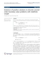
Title Suppressed Due to Excessive Length 15
hence problem (12) has a unique solution (see Figure 1) which is given by
x(t) =

t
0
dr
cos r − 3
, t ∈ [0, L].
3 Construction of lower and upper solutions
In general, condition (H
1
) is the most difficult to check among all the hy-
potheses in Theorem 1. Because of this, we include in this section some
sufficient conditions on the existence of linear lower and upper solutions for
problem (1) in particular cases We begin by considering a problem of the
form







x

(t) = f (x(τ (t, x))) for a.a. t ∈ I
0
= [t
0

, t
0
+ L],
x(t) = k(t) for all t ∈ I
−
= [t
0
− r, t
0
],
(13)
where f ∈ C(R) and k ∈ C(I
−
).
16 Rub´en Figueroa
∗
and Rodrigo L´opez Pouso
Proposition 1 Assume that f is a continuous function satisfying
lim
y→+ ∞
f(y) = +∞; (14)
lim
y →−∞
f(y) = −∞; (15)
lim
y →±∞
f(y)
y
<
1

L
. (16)
Then there exist m, m > 0 such that the functions
α(t) =







ϕ
∗
, if t < t
0
,
m(t
0
− t) + ϕ
∗
, if t ≥ t
0
,
(17)
and
β(t) =








ϕ
∗
, if t < t
0
,
m(t − t
0
) + ϕ
∗
, if t ≥ t
0
,
(18)
are, respectively, a lower and an upper solution for problem (13), where
ϕ
∗
= min
t∈I
−
k(t), ϕ
∗
= max
t∈I
−
k(t).
In particular, problem (13) has maximal and minimal solutions between
α and β, and this does not depend on the choice of τ.

Proof. Conditions (15) and (16) imply that
lim
y→−∞
y − ϕ
∗
f(y)
> L,
so there exists y
1
< min{0, ϕ
∗
} such that
0 > f (y) >
y − ϕ
∗
L
if y ≤ y
1
. (19)
On the other hand, condition (14) implies that there exists y
2
> 0 such that
f(y) > 0 if y ≥ y
2
. (20)
Title Suppressed Due to Excessive Length 17
Let λ = min{f(y) : y
1
≤ y ≤ y
2

}. By condition (15) and continuity of
f, there exists y
3
≤ y
1
such that
f(y
3
) = λ and f(y) ≥ λ for all y ∈ [y
3
, y
1
], (21)
and this choice of y
3
also provides that
f(y
3
) ≤ f (y) for all y ≥ y
3
, (22)
and, by virtue of (19),
f(y
3
) >
y
3
− ϕ
∗
L

. (23)
Now, define α as in (17), with m =
ϕ
∗
−y
3
L
. Notice that α(t) ≤ k(t) for
all t ∈ I
−
, α

(t) =
y
3
−ϕ
∗
L
for all t ∈ I
0
and
min
t∈I
α(t) = α(t
0
+ L) = −mL + ϕ
∗
= y
3
,

so we deduce from (22) and (23) that for all t ∈ I
0
we have
α

(t) = −m < f (y
3
) = min
y ≥ min
I
α(t)
f(y). (24)
In the same way, we can find y
3
≥ max{0, ϕ
∗
} such that β defined as in
(18) with m =
ϕ
∗
−y
3
L
satisfies that β (t) ≥ k(t) for all t ∈ I
−
and
β

(t) = m ≥ max
y ≤max

I
β(t)
f(y) for all t ∈ I
0
. (25)
So we deduce from (24) and (25) that α and β are lower and upper
solutions for problem (13). 
18 Rub´en Figueroa
∗
and Rodrigo L´opez Pouso
Example 4 The function
f(y) =







sgn(y) log |y|, if y ∈ (−∞, −1) ∪ (1, ∞),
sin(πy), if y ∈ [−1, 1],
satisfies all the conditions in Proposition 1 for every compact interval I
0
.
So the corresponding problem (13) has at least one solution for any choice
of k ∈ C(I
−
) and τ ∈ C(I, I).
We use now the ideas of Proposition 1 to construct lower and upper
solutions for the general problem (1).

Proposition 2 Let k ∈ C(I
0
) and let f : I
0
× R
2
−→ R be a Carath´eodory
function. Assume that there exist F
α
, F
β
∈ C(R) such that for a.a. t ∈ I
0
and al l y ∈ R we have
f(t, x, y) ≥ F
α
(y) for all x ≤ ϕ
∗
(26)
and
f(t, x, y) ≤ F
β
(y) for all x ≥ ϕ
∗
. (27)
Moreover, assume that the next conditions involving F
α
and F
β
hold:

lim
y →−∞
F
α
(y) = −∞, (28)
F
α
is bounded from below in [0, +∞), (29)
lim
y →−∞
F
α
(y)
y
<
1
L
, (30)
lim
y →+ ∞
F
β
(y) = +∞, (31)
F
β
is bounded from above in (−∞, 0], (32)
lim
y →+∞
F
β

(y)
y
<
1
L
. (33)
Title Suppressed Due to Excessive Length 19
Then there exist m, m ≥ 0 such that α and β defined as in (17), (18)
are lower and upper solutions for problem (1) with Λ = 0, and this does not
depend on the choice of τ.
Proof. Reasoning in the same way as in the proof of Proposition 1, we
obtain that there exists m ≥ 0 such that α(t) ≤ ϕ
∗
for all t ∈ I
−
and
α

(t) = −m ≤ min
y ≥ min
I
α
F
α
(y) for a.a. t ∈ I
0
.
As α (t) ≤ ϕ
∗
for all t ∈ I, we obtain by virtue of (26) that

α

(t) ≤ min
y ≥ min
I
α
f(t, α(t), y) for a.a. t ∈ I
0
.
In the same way, there exists m ≥ 0 such that β(t) ≥ ϕ
∗
for all t ∈ I
−
and
β

(t) = m ≥ max
y ≤max
I
β
f(t, β(t), y) for a.a. t ∈ I
0
.
Therefore, α and β are lower and upper solutions for problem (1). 
Example 5 Let F be the function defined in Example 4 and consider the
problem








x

(t) = −(x + π)|x + π|
γ
g(t, x) + F (x(τ(t, x))) for a.a. t ∈ [0, L],
x(t) = −t cos t for all t ∈ [−π, 0],
(34)
where γ ≥ 0, L > 0, and g is a nonnegative Carath´eodory function.
In this case, we have ϕ
∗
= −π , ϕ
∗
≈ 0.5611, and the function f(t, x, y)
which defines the equation satisfies
f(t, x, y) ≥ F (y) if x ≤ −π and f(t, x, y) ≤ F (y) if x ≥ −π,
20 Rub´en Figueroa
∗
and Rodrigo L´opez Pouso
so in particular conditions (26) and (27) hold. As conditions (28)–(33) also
hold (see Example 4) we obtain that there exist m, m > 0 such that α and
β defined as in (17), (18) are lower and upper solutions for problem (34) for
any choice of τ. In particular, if there exists ψ ∈ L
1
(I
0
) such that for a.a.
t ∈ I

0
and all x ∈ [α(t), β(t)] we have g(t, x) ≤ ψ(t), then problem (34) has
maximal and minimal solutions between α and β.
Remark 3 Notice that the lower and upper solutions obtained both in Propo-
sitions 1 and 2 satisfy a slightly stronger condition than the one required in
Definition 1.
Competing interests
The authors declare that they have no competing interests.
Authors’ contributions
Both authors’ contributions to this paper are similar and it is impossible
to say which part corresponds to each author’s work. All authors read and
approved the final manuscript.
Acknowledgement
This study was partially supported by the FEDER and Ministerio de Edu-
caci´on y Ciencia, Spain, project MTM2010-15314.
Title Suppressed Due to Excessive Length 21
References
1. Figueroa, R, Pouso, RL: Minimal and maximal solutions to second-order
b oundary value problems with state-dep endent deviating arguments Bull.
Lond. Math. Soc. 43, 164–174 (2011)
2. Arino, O, Hadeler, KP, Hbid, ML: Existence of periodic solutions for delay
differential equations with state dependent delay. J. Diff. Equ. 144(2), 263–
301 (1998)
3. Dyki, A: Boundary value problems for differential equations with deviated
arguments which depend on the unknown solution. Appl. Math. Comput.
215(5), 1895–1899 (2009)
4. Dyki, A, Jankowski, T: Boundary value problems for ordinary differential
equations with deviated arguments. J. Optim. Theory Appl. 135(2), 257–269
(2007)
5. Jankowski, T: Existence of solutions of boundary value problems for dif-

ferential equations in which deviated arguments depend on the unknown
solution. Comput. Math. Appl. 54(3), 357–363 (2007)
6. Jankowski, T: Monotone method to Volterra and Fredholm integral equa-
tions with deviating arguments. Integ. Transforms Spec. Funct. 19(1–2),
95–104 (2008)
7. Walther, HO: A periodic solution of a differential equation with state-
dep endent delay. J. Diff. Equ. 244(8), 1910–1945 (2008)
8. Hartung, F, Krisztin, T, Walther, HO, Wu, J: Functional differential
equations with state-dependent delays: theory and applications. Hand-
b ook of Differential Equations: Ordinary Differential Equations, vol. III.
Elsevier/North-Holland, Amsterdam (2006), pp. 435–545
22 Rub´en Figueroa
∗
and Rodrigo L´opez Pouso
9. Cid, J
´
A: On extremal fixed points in Schauder’s theorem with applications
to differential equations. Bull. Belg. Math. Soc. Simon Stevin 11(1), 15–20
(2004)
Fig. 1 Solution of (12) bracketed by the lower and the upper solution.
Figure 1