Báo cáo hóa học: " Pipeline synthesis and optimization of FPGAbased video processing applications with CAL" pot

RESEARCH Open Access
Pipeline synthesis and optimization of FPGA-
based video processing applications with CAL
Ab Al-Hadi Ab Rahman
*
, Anatoly Prihozhy and Marco Mattavelli
Abstract
This article describes a pipeline synthesis and optimization technique that increases data throughput of FPGA-
based system using minimum pipeline resources. The technique is applied on CAL dataflow language, and
designed based on relations, matrices, and graphs. First, the initial as-soon-as-possible (ASAP) and as-late-as-
possible (ALAP) schedules, and the corresponding mobility of operators are generated. From this, operator coloring
technique is used on conflict and nonconflict directed graphs using recursive functions and explicit stack
mechanisms. For each feasible number of pipeline stages, a pipeline schedule with minimum total register width is
taken as an optimal coloring, which is then automatically transformed to a description in CAL. The generated
pipelined CAL descriptions are finally synthesized to hardware description languages for FPGA implementation.
Experimental results of three video processing applications demonstrate up to 3.9× higher throughput for
pipelined compared to non-pipelined implementations, and average total pipeline register width reducti on of up
to 39.6 and 49.9% between the optimal, and ASAP and ALAP pipeline schedules, respectively.
1 Introduction
Data throughput is one of the most important para-
meters in video processing systems. It is essentially a
measure of how fast data passes from inpu t to output of
a system. With increasing demands for larger resolution
images, faster frame rates, and more processing require-
ments through advanced algorithms, it is becoming a
major challenge to m eet the ever-increasing desirable
throughput.
For algorithms that can be performed in paral lel, such
as the case with most digital signal processing (DSP)
applications, parallel platf orms such as multi-core CPU,
many-core GPU, and FPGA generally results in higher

throughput compared to traditional single-core systems.
Among these parallel platforms, FPGA systems allow
the most parallel operations with the highest flexibility
for programming parallel cores. However, register trans-
fer level (RTL) designs for FPGA are known to be diffi-
cult and time consuming, especially for complex
algorithms [1]. As time-to-market window continues to
shrink, a new high-level program that synthesizes to effi-
cient parallel hardware is required to manage complex-
ity and increase productivity.
The CAL dataflow language [2] was developed to
address these issues, specifically with a goal to synthe-
size high-level programs into effici ent parallel ha rdware
(see Section 3.2). CAL is an actor language in which
program executes based on tokens; therefore, suitable
for data intensive algorithms such as in DSP that oper-
ates o n multiple data. The language was also chosen by
the ISO/IEC
a
as a language for the description and spe-
cification of video codecs.
CAL design environment was initiated and developed
by Xilinx Inc. and later became Eclipse IDE open source
plugins called Ope nDF and OpenForge [3] w hich allow
designers to simulate CAL models and synthesize to
hardware description languages (HDL). The tools only
perform basic optimizatio ns for a given CAL actor for
HDL synthesis; the final result highly depends on the
design style and specification. Reference [4] presents
coding recommendations for CAL designers to achieve

best results. However, some optimizations are best per-
formed automatically rather than manually, for example
pipeline synthesis and optimization of CAL actors.
In CAL designs, actions execute in a single-clock cycle
(with exception to while loops and m emory access).
Large actions, therefore, would result in a large combi-
natorial logic and reduces the maximum allowable oper-
ating frequency which in turn decreases throughput.
* Correspondence:
SCI-STI-MM, Ecole Polytechnique Fédérale de Lausanne, 1015 Lausanne,
Switzerland
Ab Rahman et al. EURASIP Journal on Image and Video Processing 2011, 2011:19
/>© 2011 Ab Rahman et al; licensee Springer. This is an Open Access article d istributed under the terms of the Creative Commons
Attribution License ( which permits unrestricted use, distribution, and reprodu ction in
any medium, pro vided the original work is properly cited.
The pipeline o ptimization strategy is to partition this
large action into smaller actions that satisfy a required
throughput requirement, but with a minimum resource
penalty. Finding a pipeline schedule that minimizes
resource is a nonlinear optimization problem, where the
number of poss ible solutions increase s exponentially
with a linear increase of operator mobility.
This study presents an automatic non-pipelined CAL
actor transformation to re source-optimal-pipelin ed CAL
actors that meet a required stage-time constraint. The
objective is to all ow designers to rapidly design complex
DSP hardware systems usingCALdataflowlanguage,
and use our tool to obtain higher throughput with opti-
mized resources by pipelining the longest action in the
design. In o rder to evalua te the efficiency of our metho-

dology, three video processing algorithms are designed
and used for pipeline synthesis and optimization.
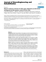
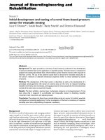
Figure 1 shows CAL to HDL design flow methodology
with our CAL to CAL pipeline optimization strategy.
Starting with an initial CAL design, it is first synthesized
to HDL, then to a specific FPGA technology where the
critical path and maximum allowable frequency infor-
mation can be obtained. If the throughput requirement
is met, the design can be implemented directly into the
FPGA. In the case when a higher throughput i s
required, the action with the critical path is extracted
from the design, and automatically pipelined with the
required delay (for that actor) with minimum resource
penalty. The original non-pipelined CAL actor is then
replaced by the newly generated pipelined CAL actors.
This process is repeated until the desired system
throughput is achieved.
This article is organized as follows. The next section
provides background and related study on pipeline
synthesis and optimizations. Section 3 presents the
basics of dataflow modeling in CAL. Following this, in
Sections 4 and 5, we present our approach to pipeline
synthesis and optimization using mathematical formula-
tions. Then, in Section 6, experimental results are
shown for several video processing applications, and
finally, the last section concludes the article.
2 Pipeline synthesis and optimization:
background
In computing, a pipeline is a set of data processing ele-
ments connected in series, so that the output of one ele-

ment is the input of the next one. The elements of a
pipeline are executed in parallel or in time-sliced fash-
ion; in this case, some amount of buffer storage (pipe-
line registers) is inserted in between elements. The time
between each clock signal is set to be greater tha n the
longest delay between pipeline stage s, so that when the
registers are clocked, th e data that is written to the fol-
lowingregistersisthefinalresult of the previous stage.
A pipelined system typically requires more resources
(circuit elements, processing units, computer memory,
etc.) than one that executes one batch at a time, because
each pipeline stage cannot reuse the resources of the
other stages.
Key pipeline parameters are number of pipeline stages,
latency, clock cycle time, delay, turnaround time, and
throughput. A pipeline synthesis problem can be con-
strained either by resource or time, or a combination of
both [5]. A resource-constraint pipeline synthesis limits
the area of a chip or the available number of functional
units of each type. In this case, the objective of the schedu-
ler is to find a schedule with maximum p erformance,
given available resources. On the other hand, a time-con-
straint pipeline synthesis specifies the required throughput
and turnaround time, with the objective of the scheduler
is to find a schedule that consume minimum resources.
Sehwa [6] is the first pipeline synthesis program. For a
given constraint on the number of resources, it imple-
ments a pipelined datapath with minimum latency.
Sehwa minimizes time delay using a modified list sche-
duling algorithm with a resource allocation table. HAL

[7] performs a time-constrained, functional pipelining
scheduling using the force directed method which is
modified in [8]. The loop winding method was proposed
in the Elf [9] system. A loop iteration is partitioned hor-
izontally into several pieces, which are then arranged in
parallel to achieve a higher throughput. The percola-
tion-based scheduling [10] deals with the loop winding
by starting with an optimal schedule [11] which is
obtained without considering resource const raints. Spaid
[12] finds a maximally parallel pattern using a linear
programming formulation. ATOMICS [13] per forms
loop optimizatio n starting with estimating a latency and
inter-iteration precedence. Operations which ca nnot be
scheduled within the latency are folded to the next
iteration, the latency is decreased, and the folding is
applied again. The above-listed tools support r esource
sharing during pipeline optimization.
SODAS [14] is a pipelined datapath synthesis system
targeted for application-specific DSP chip design. Taking
signal flow graphs (SFG) as input, SODAS-DSP gener-
ates pipel ined datapaths through iteratively constructive
variation of the list scheduling and module allocation
processes that iteratively improves the i nterconnection
cost, where the measure of equid istribution of opera-
tions among pipeline partitions is adopted as the objec-
tive function. Area and performance trade-off in
pipel ine designs can be achieved by changing the synth-
esis parameters, data initiation interval, clock cycle time,
and number of pipeline stages. Through careful schedul-
ing of operations to pipeline stages and allocation of

hardware modules, high utilization of hardware modules
can be achieved.
Ab Rahman et al. EURASIP Journal on Image and Video Processing 2011, 2011:19
/>Page 2 of 28
Pipelining is an effective method to optimize the
execution of a loop with or without loop ca rried depen-
dencies, especially for DSP [8]. Highly concurrent imple-
mentations can be obtained by overlapping the
execution of consecutive iterations. Forward and back-
ward scheduling is iteratively used to minimize the delay
in order to have more silicon area for allocating addi-
tional resources which in turn will increase throughput.
Figure 1 CAL to HDL design flow with the proposed CAL to CAL pipeline optimization strategy.
Ab Rahman et al. EURASIP Journal on Image and Video Processing 2011, 2011:19
/>Page 3 of 28
Another important concept in circuit pipelining is
Retiming, which exploits the ability to move registers in
the circuit in order to de crease the length of the longest
path while preserving its functional behavior [15-17]. A
sequential circuit is an interconnection of l ogic gates
and memory elements which communicate with its
environment through primary inputs and primary out-
puts. The performance optimization problem of pipe-
lined circuits is to maximize the clocking rate or
equivalently minimize the cycle time of the circuit. The
aim of constrained min-area retiming is to constrain the
number of registers for a target clock period, under the
assumption that all registers have the same area, the
min-area retiming problem reduces to seeking a solution
with the minimum number of registers in the circuit. In

the retiming problem, the objective function and con-
straints are linear, so linear programming techniques
can be used to solve this problem. The basic version of
retiming can be solved in polynomial time. The concept
of retiming propo sed by Leiserson et al. [15] was
extended to peripheral retiming in [16] by introducing
the concept of a “negative” register. These studies
assume that the degree of functional pipelining has
already been fixed and consider only the problem of
adding pipeline buffers to improve performance of an
asynchronous circuit.
The studies discussed are mainly targeted at the gen-
eration and optimization of hardware resources from
behavioral RTL descriptions. As to our knowledge, there
is no available tool that performs these functions at the
level of a dataflow program. The recent development of
the CAL dataflow language allows the application of
these techniques at a higher abstractio n level, thu s pro -
vide the advantages of rapid design space exploration to
explore pipeline throughput and area trade-off, and sim-
pler transformation of a non-pipelined to a pipelined
behavioral description, compared to low abstraction
level RTL. The next section presents background on
dataflow networks, high-level modeling for hardware
synthesis, and the CAL actor language.
3 Dataflow modeling and high-le vel synthesis
Early studies on dataflow modeling are based on the
Kahn process network introduced by Kahn in 1974 [18],
which is a dataflow network with a local sequential pro-
cess and global concurrent processes. This has been

extended to graph models with a number of variants
such as the directed acyclic graphs (DAG) [19-21]
whereeachnoderepresentsanatomicoperation,and
edges represent data dependencies. The extension of the
DAG is the synchronous dataflow graphs (SDF) [22]
that annotates the number of tokens produced and con-
sumed by the computation node, thus allowing feasible
actor scheduling. Another type of dataflow graph is the
control dataflow graphs ( CDFG) [23] which describes
static control flow of a program using the concept of a
director that regulates how actors in the design fire and
how tokens are used.
Several dataflow implementation methodologies have
been proposed to use pre-configured IP blocks in a data-
flow environment such as the PICO framework [24], sim-
pleScalar [23], and the study of Lahiri et al. [25]. There
exist also commercial tools to aid DSP hardware designs
such as Cadence SPW [26], Altera DSP Builde r [27] and
Xilinx AccelDSP [28]. Some of these offer integration
with Mathworks MATLAB and SIMULINK [29]. These
methods, however, constraint the design to a given class
of architecture and put restrictions on designers.
In contrast to block-based DSP, C language, on the
other hand, offers higher flexibility. Synthesis from C to
hardware has been a topic of intensive research with
developments such as the Spark framework [30], GAUT
tool of LABSTICC [31], and Catapult C from Mentor
Graphics [32]. However, C program is designed to exe-
cute sequentially, and it still remains a diffic ult problem
to generate efficient HDL codes from C, especially for

DSP applications. Furthermore, C programs are also dif-
ficult to analyze and identify for potential parallelism
because of the lack of concurrency and the conce pt of
time [33]. In the context of RTL, SystemC was intro-
duced but mainly restricted to system level simulations
and offered limited support for hardware synthesis.
Transaction level modeling raises the a bstraction level
one step above systemC, and has gai ned popularity, but
the level of abstraction remains quite low for effective
designs.
High-level synthesis methodologies have also been
used to generate pipeline schedules in RTL, for example
in [34], where a variation of the Modulo scheduling
algorithm has been used to exploit loop-parallelism b y
means of executing operations from consecutive itera-
tions of a loop in parallel. The technique is applied on
the level of an assembly language for generating pipe-
lined RTL descrip tions. However, besides the limitation
of the technique on loop algorithms, the level of the
input descriptio n is sequential and again, faces the ana-
lyzability problem for effective pipelining. The study
reported an improvement of up t o 35% between pipe-
lined and non-pipelined implementations.
In order to overcome these issues in the state of the
art of high-level modeling and synthesis, the Ptolemy
project at the University of California-Berkeley led to
the development of the CAL dataflow language based
on the concept of actors.
3.1 Actor-based dataflow modeling
Actors were first introduced in [35] as means of model-

ing distributed knowledge-based algorithms. Actors have
Ab Rahman et al. EURASIP Journal on Image and Video Processing 2011, 2011:19
/>Page 4 of 28
since then become widely used [1-4,36-41], especially in
embedded systems, where actor-oriented design is a nat-
ural match to the hetero geneous and concurrent nature
of such systems.
Many embedded systems have significant parts that
are best c onceptualized as dataflow systems, in which
actors execute and communicate by sending each other
packets of data. It is often useful to abstract a syst em as
a structure of cooperating actors. Many such systems
are dataflow-oriented, i.e. they consist of components
whose ability t o perform computation depends on the
availability of sufficient input data. Typical signal pro-
cessing systems, and also many control systems fall into
this category.
Component-based design is an approach to software
and system engineering, in which new software designs
are created by combining pre-existing software compo-
nents. Actor-oriented modeling is an approach to sys-
tems design, where entities called actors communicate
with each other through ports and communication chan-
nels. From the point of view of component-based design,
actors are the components in actor-oriented modeling.
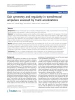
Figure 2 shows a simple dataflow network. Several
actors are composed into a network, a graph-like struc-
ture (often referred to as a model) in which output
ports of ac tors are connected (typically with FIFO buf-
fers) to input ports of the same or other actors, indicat-

ing that tokens produced at those output ports are to be
sent to the corresponding input ports. Such actor net-
works are of course essential to the construction of
complex systems. The encapsulation of each actor
means that they are treated as a separate entity that
works independently, but concurrently in a network.
Increasing the number of actors in the network implies
more concurrent operations; which is analogous to
pipelining.
3.2 CAL dataflow language
CAL is a domain-specific language for writing dataflow
actors, with the final language specification released at the
end of 2003 [36]. The language describes an algorithm
using an encapsulated actor, which communicates with
another actor by passing data tokens. An actor then per-
forms its algorithm specified in its action if there is token
available and if it is enabled by one or more of the follow-
ing: guard, priority,andscheduling conditions. If an action
is performed, it is said to be fired, which consumes the
input token, modify its internal states (variables, guard,
schedule) and produces an output token which can be
passed to another actor, itself or the system output [2]. An
example of a CAL actor is given in Section 4.
CAL, however, is not a general purpose or full-fledged
programming lan guage; one o f its key goals is to make
actor programming easier by providing a concise high-
level description with explicit dataflow keywords, unlike
traditional progr amming languages. It is also designed to
be platform independent and retargetable to a rich variety
of target platforms, for example single-core and multi-core

CPUs [1,36,41], FPGAs [1,37,39], and ASICs [38]. CAL
provides a strict semantics for defining actor computa-
tional operations, ports and parameters and its composite
data structures. But it leaves certain issues to the embed-
ding environment, such as the choice of supported data
types and the definition of the target semantics.
3.3 CAL to HDL synthesis
The synthesis of CAL program to HDL is one of the core
components o f the CAL dataflow language. It was
Figure 2 Dataflow network with actors, tokens, and buffers.
Ab Rahman et al. EURASIP Journal on Image and Video Processing 2011, 2011:19
/>Page 5 of 28
pioneered by Xilinx Inc. and now available as Eclipse IDE
opensource plugins called OpenDF and OpenForge [3].
The CAL to HDL code generator is essentially an XML
processing and transformation engine using Java. The two
main steps are:
1. Generation of top level VHDL from a flattened
CALdataflow network. The tool takes in a flattened
CAL network called XDF, and transforms it into a
top-level VHDL file. Some of the operations include
port evaluation, data width, fanout, and buffer size
annotation, and instance name addition.
2. Generation of Verilog files for each CALactor.CAL
actors are first checked synta ctically, and then parsed
into various XML representations that include several
basic optimization steps. The final XML representation
is called SLIM, which is a representation in a s ingle-sta-
tic assignment (SSA
b

) form. SLIM file is then loaded
into a Java Design class that represents top-level hard-
ware implementation. The Java object representing the
actor is optimized for hardware which includes opera-
tor constant rule, loop unrolling, variable re-sizer,
memory reducer, splitter and trimmer. Next, a hard-
ware scheduler is also generated based o n the specifica-
tion in the SLIM representation. Finally, a completed
design object for an actor is written a s a Verilog file.
HDL c ode generation from CAL actors has proven to
generate efficient ha rdware. As reported in [37] for the
hardware implementation of MPEG-4 Simple Profile
Decoder, CAL design results in less coding, smaller
implementation area, and higher throughput compared
to classical RTL methodology.
The strength of the CAL dataflow language, especially
for parallel DSP application, and its HDL synthesis makes
it interesting for further optimization. As described, the
CAL to HDL synthesis tool optimizes and generates code
for each actor; no study has been done on actor partition-
ing for pipelining, which is the focus of this article.
4 Mathematical modeling of pipeline synthesis
and optimization
In order to clearly present our mathematical formula-
tion of the pipeline synthesis and optimization, the theo-
retical model will be complemented with a simple
example–the YCrCb to RGB converter actor. A brief
introduction to this actor will be given first.
4.1 The YCrCb to RGB conversion actor
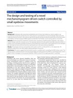
Figure 3 shows a CAL description of a 30-bit YCrCb to

24-bit RGB, based on Xilinx XAPP930 [42]. It is typi-
cally used in high quality down-sampling and decoding
of color spaces. The actor contains a single action that
firstconverts10-bitinputsintoanexplicit11-bit
unsigned representation using the bitand operation. Fol-
lowing this, the cor e algorithm is performed using 11
adders/subtractors, 4 multipliers, and 6 shifters. Finally,
the RGB output has to be clipped if the result exceeds
the 8-bit per output dynamic range. This utilizes six if
statements with comparators.
The general idea in our pipeline synthesis is to parti-
tion this relatively large action into several actions in
separate actors. The first step is to make the action
body (i.e. operations) more analyzable. This is achieved
by limiting each arithmetic operator to two operands,
and assigning a unique output variable for each opera-
tor, essentially transforming each operator to a two-
operands-single-assignment form. The dataflow graph of
this transformation is given in Figure 4. Twenty extra
variables (z1 to z20) are introduced to represent inter-
mediate results of 35 operations.
The remainder of this section provides relations,
graphs, and algorithms that define pipeline synthesis
and optimization problem from a generic dataflow
graph, with an example using the graph of Figure 4.
4.2 Dataflow graph relations
4.2.1 Operator precedence relation on dataflow graph
Let N = {1, , n} be a set of algorith m operators and M =
{1, , m} be a set of algorithm variables. The following
actor YCrCbtoRGB ( )

in t ( s i z e =10) Y, in t ( si z e =10) Cr , i n t ( s i z e =10) Cb ⇒
int (size=8) R, int (size =8) G, int( size=8) B :
in t ( s i z e =13) r v = 292;
i n t ( s i z e =13) gu = 10 1;
in t ( s i z e =13) gv = 1 49 ;
in t ( s i z e =13) bu = 52 0;
int ( size =11) t1 := 1023;
action
Y:[y], Cr:[cr], Cb:[cb] ⇒
R:[r], G:[g], B:[b]
var
in t ( s i z e =10) r , in t ( si z e =10) g , i n t ( s i z e =10) b , i n t ( s i z e =10) r t ,
in t ( s i z e =10) g t , in t ( si z e =10) bt , int ( s i z e =11) yt , in t ( si z e =11)crt
,
in t ( s i z e =11) cbt
do
// sign ed to unsigned repre sen tat ion
yt := bitand (y, t1 );
crt := bitand (cr , t1 );
cbt := bitand (cb , t1);
//c o r e a l gorit hm
rt := ((( yt−64) << 8) + rv ∗ (crt− 512)) >> 10;
gt := (((yt− 64) << 8) − gu ∗ (cbt− 512) − gv ∗ (crt− 512)) >> 10;
bt := (((yt− 64) << 8) + bu∗ (cbt− 512)) >> 10;
// clip output r
if (rt > 0) then
if (rt < 255) then r:=rt;
else r := 255; end
else
r:=0;

end
// clip output g
if (gt > 0) then
if (gt < 255) then g:=gt;
else g := 255; end
else
g:=0;
end
// clip output b
if (bt > 0) then
if (bt < 255) then b:=bt;
else b
:= 255; end
else
b:= 0;
end
end
end
Figure 3 CAL actor example–actor YCrCbtoRGB.
Ab Rahman et al. EURASIP Journal on Image and Video Processing 2011, 2011:19
/>Page 6 of 28
matrices describe operator-varia ble and precedence rela-
tions.
1. The operators/input variables relation. The opera-
tors/input variables relation is described with the F
(n, m) matrix:
F =
⎡
⎢
⎣

f
1,1
··· f
1,m
.
.
.
.
.
.
.
.
.
f
n,1
··· f
n,m
⎤
⎥
⎦
,
where f
i, j
Î {0, 1} for i Î N and j Î M.Iff
i, j
=1,
then the j variable is an input for the i operator,
otherwise it is not. In the CAL l anguage, input
tokens are co nsidered as input variables of operators
in all actions of one actor.

2. The operators/output variables relation. This rela-
tion describes which variables are outputs of the
operators. It is represented with the H(n, m) matrix:
H =
⎡
⎢
⎣
h
1,1
··· h
1,m
.
.
.
.
.
.
.
.
.
h
n,1
··· h
n,m
⎤
⎥
⎦
,
where h
i, j

Î {0, 1} for i Î N and j Î M.Ifh
i, j
=1,
then the j variable is an output for the i operator,
Figure 4 Dataflow graph of the action in the YCrCbtoRGB actor in the two-operands-single-assignment form.
Ab Rahman et al. EURASIP Journal on Image and Video Processing 2011, 2011:19
/>Page 7 of 28
otherwise it is not. In the CAL language, output
tokens are considered as output variables of opera-
tors in all actions of one actor.
3. The operator direct precedence relation. This rela-
tion describes a partial order on the set of operators
derived from analysis of the data dependencies
between operators on the data flow graph. The rela-
tion is represented with the P
direct
(n, n) matrix:
P
direct
=
⎡
⎢
⎣
p
1,1
··· p
1,n
.
.
.

.
.
.
.
.
.
p
n,1
··· p
n,n
⎤
⎥
⎦
,
where p
i, j
Î {0, 1} for i, j Î N.Ifp
i, j
= 1, then the i
operator is a direc t predecessor for the j operator,
otherwiseitisnot.Usually,thisisduetothej
operator that consumes a valu e produced by the i
operator. For the single-assignment model of an
acyclic algorithm, the direct precedence is defined
over the F and H matrices as
P
direct
= H × F
t
,

(1)
where × is matrix multiplication operation, and H
t
is
a transpose of the H matrix.
4. The operator precedence relation. The direct/
indirect precedence P
total
relation between operators
can be inferred by applying the transitive closure
operation to the P
direct
(n, n) matrix:
P
total
= P
direct
∪ P
2
direct
∪···∪P
i
direct
∪···∪P
n
direct
,
(2)
where
P

i
direct
is P
direct
in power of i. We will say that
P
direct
defines the direct precedence relation and P
to-
tal
defines the precedence relation.
4.2.2 Estimation of operator delays
The operator delay depends on the method of implemen-
tation. Different implementations of the same operator
give different parameters including time delay and area
of the functional units that implement the operators.
In order to perform pipeline synthesis and optimiza-
tion,relativetimedelaymaybeused.Table1shows
relative time delay of an adder wh ich is assumed to be
1.00. T he delays of other operators are estimated com-
pared to the delay of the adder. Thus, the delay of mul-
tiplication operator is estimated to be 3. 00, and the
delay of if-operator is estimated at 0.05.
It should be noted that operator relative delays have
to be recalculated depending on the operand widths.
For example, a 32-bit variable would use a 32-bit adder,
which typically has a higher delay compared to an 8-bit
variable that only uses an 8-bit adder. For more accurate
results, operand widths have to be taken into account
when estimating operator delays.

Another issue with operator delay estimation is the
total delay on a path. The total delay along path L is
usually estimated by
delay(L)=

i∈L
delay(i).
(3)
This simpl ification can imply significant inaccuracy in
pipeline stage delay estimation. For example, if two
addition operations i and j are executed sequentially,
and each of them is implemented, for instance, by a rip-
ple carry adder, the total delay satisfies the inequality as
follows:
delay(i, j) < delay(i)+delay(j).
(4)
In order to increase the accuracy in the pipeline stage
delay estimation, a more precise technique is required
that takes into acco unt the operation implementation
methods. Furthermore, delay recalculation techniques
have to be analyzed for various operators executed
sequentially. Together with the delay recalculation based
on operand widths, technique for evaluating accurate
operator delays is an important part of the pipeline
synthesis and optimization tool.
4.2.3 Variable and register widths
In CAL programming, the following objects are possible:
constants, variables, input, and output. Their sizes
expressed in the number of bits can be defined explicitly
in the code. In the case, when a size is not defined, a

default size of 32-bit is given.
Object widths are essential parameters during hard-
ware synthesis. Extra bits may imply larger implementa-
tion area, larger delays, and reduced frequency. For this
reason, the object widths must be defined with mini-
mum possible size for a given algorithm and required
accuracy of output values. The minimum sizes can be
Table 1 CAL operator relative delays
No. CALoperator type Time delay
1 +/- 1.00
3 * 3.00
4 >/< 0.10
6 bitand/bitor 0.02
8 not 0.01
11 if 0.05
12 other
Ab Rahman et al. EURASIP Journal on Image and Video Processing 2011, 2011:19
/>Page 8 of 28
estimated automatically by the synthesis tool or manu-
ally by the designer. The bus and register widths com-
pletely depend on the object widths. Minimization of
the object widths minimizes the total register width in
thepipelineundersynthesis. For the YCrCb to RGB
converter algorithm described in Figure 3, the object,
width, and type are given in Table 2.
4.2.4 Longest path delays between operators on acyclic
operator precedence graph
The longest path delays between operators constitute a
basis for describing pipeline execution time constraints.
We introduce the G matrix that describes the maxi-

mum time delays (critical path lengths) between opera-
torsonthedataflowgraphthatcanbederivedfrom
the analysis of the data dependencies between operators
and the operator execution times:
G =
⎡
⎢
⎣
g
1,1
··· g
1,n
.
.
.
.
.
.
.
.
.
g
n,1
··· g
n,n
⎤
⎥
⎦
,
where g

i, j
at i, j Î N is a real value. If g
i, j
=0,then
there exists no path between i and j operators on the
data flow graph, and the corresponding element of the
P
total
matrix is also equal to z ero. If g
i, j
>0,thenthere
is a path between the operators. The G matrix can be
computed from the vector of operator delays and the
P
direct
matrix. An algorit hm for evaluating longest and
shortest path on directed cyclic and acyclic graphs are
described in [43].
We present an alternative algorithm for computing
the longest path length on DAG, based on the idea that
at each step we take an operator for which the longest
path lengths of all direct predecessors are evaluated and
evaluate the longest path lengths between the taken
operator and all its predecessors in two cases:
1. as a sum of delays of the taken operator and its
direct predecessor;
2. as a sum of delay of the taken operator and the
longest path length between its direct predecessor
and the predecessors of the direct predecessor.
An example of the G matrixfortheYCrCbtoRGB

converter is shown in Figure 5. It should be noted
that the longest path between variables may also be
used for pipeline synthesis and optimization, in which
case a similar G matrix can be derived. The methodol-
ogy in this article considers path length based on
operators.
4.2.5 Operator conflict graph
For a given pipelined network, we say that T
stage
is its
stage time delay, which is the worst time d elay of one
pipeline stage. Among the pipeline stages, the operator
longest path gives maximum stage delay. In the G
matrix of the operator longest p aths in the dataflow
graph, the value g
i, j
must be less than or equals to T
stage
in order for the i and j operators to be included in one
stage. If the g
i, j
value is greater than the T
stage
, then we
say that there is a conflict between i and j,andthe
operators mus t be scheduled to different stages. Taking
such pair of operators, we obtain the operator conflict
relation for a given stage delay:
ConflictRelation =


(i, j)|i, j ∈ Nandg(i, j) > T
stage

(5)
The operator conflict relation satisfies the requirement
as follows:
ConflictRelation ⊆ PrecedenceRelation
(6)
It is obvious that if T
stage
is larger than the length of
the longest path in the algorithm, then ConflictRelation
= ⊘.Iftheinequalitydelay(i)+delay(j)>T
stage
holds for
any two adjacent operators i and j on the dataflow
graph, then ConflictRela tion = PrecedenceRelation.
Therefore, the ConflictRelation essentially depends on
the value of T
stage
. By varying the value of T
stage
we can
generate diffe rent pipelines for the same dataflow graph
description.
The ConflictRelation represents operator conflict
directed graph by means of interpreting the pairs (i, j) of
operators included in the relation as the graph edge s. It
should be noted that the conflict graph configuration
and the accuracy of the final pipeline synthesis results

ess entially dep end on the accu racy of the operator rela-
tive time delay estimation.
Similar to the G matrix, variable conflict matrix and
graph can also be obtained and used for pipeline synth-
esis and optimization.
Table 2 Object width and type in the YCrCb to RGB
converter algorithm
Object Width Type
rv, gu, gv, bu 13 Constant
t1 10 Constant
y, cr, cb 10 Input
r, g, b 8 Output
rt, gt, bt, 10 Variable
z2, z3
yt, crt, cbt 11 Variable
z1, z4, z7, z8 19 Variable
z5 17 Variable
z6 18 Variable
z9, z10, z11, z12, 1 Variable
z13, z14, z15, z16,
z17, z18, z19, z20
Ab Rahman et al. EURASIP Journal on Image and Video Processing 2011, 2011:19
/>Page 9 of 28
4.2.6 Operator nonconflict graph
By means of subtraction of the ConflictRelation from the
PrecedenceRelation, we obtain a so-called nonconflict
operator relation:
NonConflictRelation = PrecedenceRelation\ConflictRelation
(7)
In the relation, a pair (i, j) of operators does not con-

stitute a conflict because the operators may be included
in the same pipeline stage. For the operators, it is possi-
ble that stage(i)<stage(j), but it is not possible that stage
(i)>stage(j). The NonConflictRelation varies in the range
∅⊆NonCon
fl
ictRelation ⊆ PrecedenceRelatio
n
(8)
When ConflictRelation is empty then NonConflictRela-
tion equals PrecedenceRelation. When ConflictRelation is
equa l to PrecedenceRelation then NonConflict Relat ion is
empty.
4.2.7 As soon as possible (ASAP) and as late as possible
(ALAP) scheduling
ASAP and ALAP are well-known scheduling techniques
that schedule operations in a dataflow graph based on
the earliest and latest possible sequence [43]. In this
study, we use N set of operators and the
ConflictRelation to generate an ASAP (and ALAP) sche-
duling that gives the earliest (and latest) stage that each
operator can be scheduled. Tables 3 and 4 show ASAP
and ALAP scheduling results for the YCrCb to RGB
converter example for T
stage
= 4.12.
4.2.8 Mobility-based operator ordering
The ASAP and ALAP results give crucial information on
the mobility of an operator, which is defined as its possibi-
lity to be scheduled to various pipeline stages. We call the

earliest stage that an operator i may be scheduled as asap
(i), and the latest as alap(i). Hence, the mobility of opera-
tor i is given by alap(i)-asap(i).Ifanoperatormaybe
scheduled to only one stage, then the mobility equals to
zero. Table 5 shows the mobility of each operator for the
YCrCb to RGB converter example for T
stage
= 4.12. The
two non-zero mobility operators, 1 and 4, imply that they
can be moved to either pipeline stage-1 or stage-2. The
optimization problem is then to determine which of the
solutions give optimal results. The next section formulates
the optimization problem.
4.3 Pipeline optimization tasks
Let N = {1, , n} be a set of algorithm operators and K
= {1, , k}beasetofpipelinestages.Thenumberof
Figure 5 Longest operator path lengths of the YCrCb to RGB converter.
Table 3 ASAP schedule for the YCrCb to RGB converter for T
stage
= 4.12
Stage Operators
1 1,2,3,4,5,6,7,8,9,10
2 11, 12, 13, 14, 15, 16, 17, 18, 19, 20, 21, 22, 23, 24, 25, 26, 27, 28, 29, 30, 31, 32, 33, 34, 35
Ab Rahman et al. EURASIP Journal on Image and Video Processing 2011, 2011:19
/>Page 10 of 28
pipeline stages is determined by the stage time delay
T
stage
. Variations in the stage d elay imply variations in
the pipeline stage count. We describe the distribution of

operators onto pipeline stages with the X matrix:
X =
⎡
⎢
⎣
x
1,1
··· x
1,n
.
.
.
.
.
.
.
.
.
x
k,1
··· x
k,n
⎤
⎥
⎦
.
Inthematrix,thenumberofrowsisequaltothe
number k of pipeline stages, and the number of columns
is equal to the number n of operators. A x
i, j

Î {0, 1}
variable for i Î N and j Î K takes one of two possible
values. If x
i, j
= 1, then the i operator is scheduled to
the j stage, otherwise it is not scheduled to the stage.
The X matrix describes a distribution o f the operators
on the stages.
In some cases, the x
i, j
variable can be determined in
advance. For example, if 1 ≤ i < asap(j), then x
i, j
=0.
Similarly, x
i, j
= 0 for alap(j)<i ≤ n.Ifi = asap(j)=alap
(j), then x
i, j
= 1. In order to develop efficient synthesis
and optimization techniques, we replace the variables
with their known values in the X matrix. The rest of the
unas signed variables may be replaced with values 0 or 1
in such a way as to obtain a valid X matrix. One X
matrix describes one possible pipeline schedule. The
upper bound S
upper
of the total number of X matrix can
be estimated as
S

upper
=

j∈N
μ(j),
(9)
where μ(j) is the number of variables with unknown
values in the j column of the X matrix.
For t he YCrCb to RGB converter example with T
stage
= 4.12, the asap and alap pipeline stages computed on
the operator conflict graph are shown in Figure 6.
Operators 1 and 4 may be scheduled to both first and
second stages. The other operators are scheduled either
to the first stage or to the second stage. The corre-
sponding X matrix is presented in Figure 7. Four e le-
ments of the matrix are variables (denoted by x), the
other elements are constants. The upper bound on the
total number of X matrix (pipelined schedules) is S
upper
=2
2
= 4. However, actual number of schedules could be
less than the upper bound since there are strong depen-
dencies among the values of the matrix variables.
4.3.1 Objective function in the optimization task
For a given T
stage
requirement, we can obtain several
pipeline schedules. Different schedules give Different

parameters. The mos t important is the number and
total w idth of registers inserted in between neighb oring
pipeline stages. Minimization of the total register width
will save the implementation area. Furthermore, the
operating frequency could also possibly be increased
with minimization of pipeline registers.
Figure 8 illustrates register usage from pipelining for
an example of a 4-stage pipeline. Between the same
stage, no registers are used since a particular stage
circuit logic is purely combinatorial (indicated by W).
Between stage k and k+1, registers are r equired if an
output of an operation in stage k is used in the fol-
lowing k+1 stage (indicated by R). If the output of
stage k is used by stage k+2 and beyond, then trans-
mission registers are required(indicatedbyT).Our
goal is to find the minimum total R and T registers
from all possible schedules for a given T
stage
constraint.
Let Ω be a set of possible X matrix. For the single-
assignment model of the source algorithm, the objective
function as follows mini mizes the total pipeline register
width over all elements of set Ω:
min
X∈
k

s=1
⎧
⎨

⎩
m

j=1
[max
i∈N
(f
i,j
× x
s,i
) − max
i∈N
(h
i,j
× x
s,i
)] × width(j)+
m

j=1
[max(τ
j
,max
e=s+1, ,k,i∈N
(f
i,j
× x
e,i
)) − max
e=s, ,k,i∈N

(h
i,j
× x
e,i
)] × width(j)
⎫
⎬
⎭
,
(10)
where τ
j
=1ifthej variable is an output token and τ
j
= 0 otherwise; × is the arithmetic multiplication
operation.
There are two parts in Equation 10. The first one esti-
mates for each stage s the width of registers inserted in
between the stage and the previous neighboring stage.
The second one estimates for each stage the width of
transmission registers.
Table 4 ALAP schedule for the YCrCb to RGB converter for T
stage
= 4.12
Stage Operators
1 2,3,5,6,7,8,9,10
2 1, 4, 11, 12, 13, 14, 15, 16, 17, 18, 19, 20, 21, 22, 23, 24, 25, 26, 27, 28, 29, 30, 31, 32, 33, 34, 35
Table 5 Operator mobility for the YCrCb to RGB converter for T
stage
= 4.12

Mobility Operators
0 2, 3, 5, 6, 7, 8, 9, 10, 11, 12, 13, 14, 15, 16, 17, 18, 19, 20, 21, 22, 23, 24, 25, 26, 27, 28, 29, 30, 31, 32, 33, 34, 35
11,4
Ab Rahman et al. EURASIP Journal on Image and Video Processing 2011, 2011:19
/>Page 11 of 28
4.3.2 Optimization task constraints
There are three constraints related to our optimization
tasks–operator scheduling, time, and precedence
constraints.
The operator scheduling constraint describes the
requirement that each operator should belong to only
one pipeline stage:
alap(i)

s=asap(i)
x
s,i
=1 fori ∈ N,
(11)
where s is a pipeline stage from the rang e asap(i) to
alap(i).
The time constraint describes the requirement that
the time delay between two operators i and j must not
be larger than T
stage
if the operators are scheduled to
one pipeline stage s:
x
s,i
× x

s,j
× g
i,j
≤ T
stage
for i, j ∈ N and s ∈ K,
(12)
where g
i, j
is the longest path between i and j opera-
tors on the algorithm dataflow graph. It is easy to see
tha t if the operato rs are in the same stage and x
s, i
= x
s,
j
= 1, then the inequality as follows must hold: g
i, j
≤
T
stage
. If the operators are not in the same stage, then
the longest path length may be larger than the stage
delay.
The operator precedence constraint describes the
requirement that if the i operator is a predecessor of the
j operator on a dataflow graph, then i must be sched-
uled to a stage whose number is not greater than the
number of stage which j operator is scheduled to
a

l
ap
(
i
)

s=asap
(
i
)
(s × x
s,i
) −
a
l
ap
(
j
)

s=asap
(
j
)
(s × x
s,j
) ≤ 0 for (i, j) ∈ PrecedenceRelation
,
(13)
where PrecedenceRelation ⊆ N × N is described by the

P
total
matrix. Constraints 11, 12, and 13 together define
the structure of the optimization space.
4.3.3 Operator conflict and nonconflict directed graphs
coloring
The constraints formulated in the previous section
describe the rules that must b e followed to generate a
valid pipeline schedule. For each pipeline schedule of a
given T
stage
,acoloring technique is used on the operator
conflict and nonconflict graphs to assign an operator to
a particular pipeline stage. R eference [43] explains the
node coloring technique of an undirected graph G(V, E),
which colors the nodes such that no edge (i, j) Î E, i, j
Î V has two end-points with the same color. For any
two adjacent nodes i and j, the inequality as follows
holds: color(i) ≠ color(j). A chromatic number c(G)of
the undirected graph G is the minimum number of col-
ors over all possible colorings.
However, since our conflict and nonconflict graphs are
directed graphs, we introduce coloring on directed
graphs using the following additional requirement: for
directed edge (i, j) Î E the inequality as follows should
hold: color(i)<color(j). In the pipeline optimization task,
if the directed operator conflict graph has a chromatic
number c(G), then the pipeline can be constructed on c
( G) stages. We reduce the problem of purely directed
graph chromatic number to the problem of longest

directed path length in the operator conflict graph. This
problem has polynomial complexity.
Node coloring of the YCrCb to RGB conver ter opera-
tor conflict graph is illustrated in Figure 9. The longest
node path length equals to 2, therefore the graph chro-
matic number c(G) = 2. In thi s case, two colo rs are
used for the two stages , light and dark co lors. Note that
nodes 1 and 4 are not colored since they can be colored
with either color. However, in order to check which
color combinations are valid, the nonconf lict graph also
needs to be analyzed and colored.
Compared to the operator conflict graph coloring, the
operator nonconflict directed graph G
n
(V, E
n
) is colored
in a Different way. The inequality as follows must hold:
max
i∈μ
in
(d)
color(i) ≤ color(d) ≤ min
i∈μ
out
(d)
color(i),
(14)
where d Î V, μ
in

(d)(orμ
out
(d)) is the set of adjacent
nodes of d that are incident to incoming (or outgoing)
edges of d. We may also color the nodes from range 1
to c(G), where c(G) is t he chromatic number of the
operator conflict graph. The only restriction in such
Figure 6 ASAP and ALAP pipeline stages for the scheduled operators for the YCrCb to RGB converter example with T
stage
= 4.12.
Figure 7 Operator distribution matrix for the YCrCb to RGB converter example with T
stage
= 4.12.
Ab Rahman et al. EURASIP Journal on Image and Video Processing 2011, 2011:19
/>Page 12 of 28
coloring i s that color(i) may not be larger than color(j) if
(i, j) Î E
n
. Moreover, the nonconflict graph enables col-
oring the nodes that are not colored in the conflict
graph.
Going back to the example, we can now color nodes 1
and 4 with either one of the following: node 1 with light
color and node 4 with light color; node 1 with light
color and node 4 with dark color ; node 1 with dark
color and node 4 with dark color. Note that as revealed
in the nonconflict graph in F igure 10, the coloring of
node 1 with dark color and node 4 with light color is
not valid.
5 Pipeline synthesis and optimization

methodology and algorithms
This section presents methodology and key algorithms
for our pipeline synthesis and optimization technique.
Based on the formulations described in Section 4, a pro-
gram was developed in Java under the Eclipse IDE that
transforms a non-pipelined CAL actor into pipelined
CAL actors.
The general overview is given in Figure 11. Starting
from a non-pipelined CAL actor, the matrices F, H, P
dir-
ect
, P
total
,andG as well as the list [T
min
, , T
max
]ofthe
possible stage time T
stage
values are computed. The T
min
value equals the operator highest execution time, and the
T
max
value equals the longest path weight in actor data-
flow graph. Optimization of pipelines is performed in a
loop on various stage numbers. We start with one-stage
pipeline (K = 1) and stage time T
stage

= T
max
. For the cur-
rent T
stage
, the conflict and nonconflict operator relations
and directed graphs Gc and Gnc are generated from the
G matrix and P
total
relation. The chromatic number of
the graphs is computed using a polynomial comp lexity
algorithm. If the chromatic number is larger than the
stage number K, then the successor value of T
stage
is
taken in the ascending list of stage time values. Owing to
this, we use the lowest value of T
stage
for each number K
of stages and thus generate the fastest K-stage pipeline. If
the chromatic number is larger than the stage number K,
then the predecessor value of T
stage
in the list is taken as
its current value if T
stage
>T
min
,and0 is taken other wise.
If for the updated value T

stage
<T
min
, then the optimiza-
tion result is a set of pipelined networks of CAL actors
for various stage numbers. Otherwise, t he conflict and
nonconflict graphs are generated again for an updated
value of T
stage
. In order to evaluate the operator mobility
and to perform the critical path-based arrangement of
grap h colorings, the ASAP and ALAP schedules are gen-
erated. We propose ordered vertex coloring to order the
Figure 8 Pipeline registers and wires for a 4-stage pipeline.
Ab Rahman et al. EURASIP Journal on Image and Video Processing 2011, 2011:19
/>Page 13 of 28
generation of solutions. The ver tices in the critical (long-
est) paths are colored first. Owing to this approach, pre-
ferable solutions are generated first. Among them, the
best (optimal or proximate) solution is selected using the
pipeline register total width estimated with Equation 10.
The best solution is generated with a branch and bound
algorithm and finally used to generate pipelined CAL
actors which are then synthesized to HDL for FPGA
implementation.
In the remainder of this section, key algorithms for
generating valid operator colorings on the conflict and
nonconflict directed graphs and searching for an optimal
pipeline schedule will be presented.
The technique for generating various operator color-

ings is based on recursive function and explicit stack
mechanism. Figure 12 shows a top level recursive func-
tion Reg-WidthColoringStep which is used to generate
pipeline schedules, and minimize the total pipeline reg-
ister width. The algorithm takes in three inputs:
1. asap, wh ich is an array of operators with the cor-
responding pipeline stage using the ASAP algorithm;
2. alap, which is an array of operators with the cor-
responding pipeline stage using the ALAP algorithm;
3. order, which is an array of operators ordered
according to its mobility over pipeline stages;
Figure 9 Operator conflict graph coloring for 2-stage pipeline of the YCrCb to RGB converter with T
stage
= 4.12.
Ab Rahman et al. EURASIP Journal on Image and Video Processing 2011, 2011:19
/>Page 14 of 28
and generates the following output:
1. pipelineCount, whic h is t he number of gene rated
pipelines;
2. optimalColor, which is the optimal pipeline sche-
dule as an array of operators with the corresponding
pipeline stage;
3. minRegWidth, which is the minimum total register
width of the optimal pipeline schedule.
The algorithm in Figure 12 works as follows. The
recursive function takes in an input parameter top,
which indicates the top record in the stack of operators.
Depending on the top value, the function can return the
control, generate the next complete coloring solution
and compare it with the bes t current one, choose t he

next correct color of the current operator and generate
the next record in the stack for procedure recursive call.
In the next top+1 record, the minimum and maximum
colors of the next operator are determined. If the mini-
mum color is larger than the maximum color, then
recoloring of the current operator is performed. The
computations of minimum and maximum colors f or
operators are performed for both the conflict and the
nonconflict graphs.
Figure 10 Operator nonconflict graph coloring for 2-stage pipeline of the YCrCb to RGB converter with T
stage
= 4.12.
Ab Rahman et al. EURASIP Journal on Image and Video Processing 2011, 2011:19
/>Page 15 of 28
Figure 13 shows an algorithm to estimate minimum
colors from a conflict graph. Among all operators that
are recorded in the stack as predecessors and are in
conflict relation with the given operator op, the operator
with maximum color gives the value of minC that is
returned by the algorithm as minimum color of op
operator. The computations of maximum color from a
conflict graph, minimum color from a nonconflict
Figure 11 Methodology of the pipeline synthesis and optimization technique on CAL dataflow actor.
Ab Rahman et al. EURASIP Journal on Image and Video Processing 2011, 2011:19
/>Page 16 of 28
graph, and maximum color from a nonconflict graph are
performed in a similar way. Once all operators have
been colored and a valid pipeline schedule is generated,
the total register width is estimated to evaluate the effi-
ciency of the schedule. The function totalRegister-Width

(colors) performs this, which takes in a pipeline sche-
dule, and returns the total register width. The function
sums the width of all required pipeline and transmission
registers of a pipeline schedule. From all possible pipe-
line schedules, the smallest total register width is stored
in the variable minRegWidth with the corresponding
optimal-Colors as the best schedule.
The final step is to generate CAL actors from the
optimal coloring. This is done by taking the optimalCo-
lors array, partition the opera tors a ccording to the
scheduled stage, and print the required operations, vari-
ables, registers, inputs, and outputs declarations accord-
ing to the syntax of the CAL dataflow language. The top
level XDF ne twork of pipelined CAL actors is also auto-
matically generated based on the required number o f
pipeline stages.
It should be noted that our pro gram is designed to
generate potentially all possible valid pipeline schedules
for a given T
stage
constraint, therefore results in a global
optimum solution. The number of possible schedules
depends on the mobility of operators; an algorithm with
many operators that can be moved among various stages
would generate many possible schedules, therefore could
potentiallytakealongtimetofindaglobaloptimum.
The RegWidthColoringStep function is a basic one for
cre ating modifications which would restri ct the number
of generated solutions. Thus, it is modified to a bran ch-
and-bound algorithm by means of introducing a

RegWidthLowerBound function, which estimates a lower
bound of total pipeline register width using partial
operator coloring that is recorded in the stack, and
ASAP and ALAP colorings. The number of generated
solutions is also restricted with MeetOptimizationTime-
Constraint function which takes into account the spent
CPU t ime or the number of produced partial and com-
plete colorings.
6 Experimental results
This section presents experimental results of our pipe-
line synthesis and optimization technique. Three video
processing algorithms with relatively large combinatorial
logic are selected for pipelining–they are the YCrCb to
RGB converter, 8 × 8 1D IDCT, and Bayer filter. It is
assumed that these algorithms constitute a critical path
in a larger design, therefore, by pipelining these algo-
rithms, a throughput increase can be obtained for the
overall system.
Each design starts with an initial single CAL actor
description, automatically pipelined using our tools to
obtain multiple-actor description, and synthesized to
HDL. For hardware implementation, two different 65-
nm process node FPGAs have been used; Xilinx Virtex-
5 and Altera Stratix III, synthesized using Xilinx XST
and Altera Design Compiler tools, respectively.
6.1 YCrCb to RGB converter based on Xilinx XAPP930 [42]
This design was introduced in Section 3.2 for illustrating
our methodology. A single actor was constructed that
converts YCrCb to RGB color space. The total number
of operators is 35.

The first step is to analyze valid T
stage
constraints by
determining the minimum and maximum T
stage
from the
dataflow graph (Figure 4). This is done by looking at
Table 1 for estimating the delay of operators. From the
dataflow graph, the minimum T
stage
is defined by the
multiplication operator which is equals to 3.00. The max-
imum T
stage
is defined by the longest path length, given
in Figure 5 wh ich is 6.50. As a result , a T
stage
constraint
of 3.00 synthesizes to a 3-stage pipeline, while a stage
delay of 6.50 and above gives a non-pipelined implemen-
tation. Further analysis of the dataflow graph shows
dependency of the multiplication operators to the pre-
vious operations of bitand and subtraction. Therefore, a
T
stage
of 4.12 (bitand-subtract-multiply) is the minimum
for which the pipeline would synthesize to 2-stages.
Figure 14 shows a graph of number of pipeline stages
versus T
stage

constraint. T
stage
specification of between
3.00 and 4.12 synthesizes to a 3- stage pipeline, between
4.12 and 6.50 to a 2-stage pipeline, and 6.50 and above
gives a 1-stage pipeline (i.e. non-pipelined) to obtain
best performance for a particular number of pipeline
stages, the minimum T
stage
should be selected.
The results for 2-stage and 3-stage pipelines are given
in Table 6. For T
stage
= 4.12 with a synthesis to 2-stage
pipel ine, the optimal schedule (best) results in total reg-
ister width of 83, while in the worst case, total register
width is 92. This results i n 10.8% reduction in tota l reg-
ister width. For T
stage
=3.00withasynthesisto3-stage
pipeline, minimum total register width is 122 c ompar ed
to 131 in the worst case, with a reduction of 7.4%. Note
that reduction of register widths between best and worst
case are relatively small because of the limited optimiza-
tion space for this example, with just three for e ach
pipeline stages.
All designs (best and worst cases for comparison) have
been synthesized to HDL for FPGA impl ementation.
Figures 15 and 16 show graphs of resource versus
throughput for Virtex-5 and Stratix III FPGAs, respec-

tively.ForVirtex-5,a2-stageanda3-stagepipeline
designs require roughly 3× and 3.5× more slices, respe c-
tively, compared to a non-pipelined design. Between the
best and worst case pipelined implementations, the dif-
ferenceislessthan1%becauseofthesharingofslice
Ab Rahman et al. EURASIP Journal on Image and Video Processing 2011, 2011:19
/>Page 17 of 28
registers and LUTs. In terms of throughput, the opti-
mized 2-stage and 3-stage pipelines are roughly 65%
higher compared to a non-pipelined implementation. As
for Stratix III, a slightly different result is observed.
Similar to Virtex-5, there is a very little difference in
resource between the best and the worst case pipelines.
Compared to a non-pipeline implementation, 2-stages
pipeline utilizes roughly 22% more ALUT, with 59%
higher throughput. For the 3-stage pipeline, ALUT is
increased by up to 44% with 57% more throughput.
In both FPGAs, it can be seen that the throughput is
almost similar for 2-stages and 3-stages pipeline imple-
mentations. In other words, 3-stage pipeline does not
result in significant increase in throughput compared to
a 2-stage pipeline. The reason is due to the saturation of
throughput, because at this point, the critical path is
now in the co ntrol (i.e. registers) and hardware inter-
connection rather than the operators as in the non-pipe-
lined implementation.
It should be noted that the ASAP and ALAP pipeline
schedules can also be generated and compared. However,
because of the small optimizatio n space of this design,
the ASAP pipeline schedule is found to be the same as

the worst case schedule, and ALAP to be the same as the
best case schedule. The next two examples present
designs with significantly larger optimization space.
6.2 8 × 8 1D IDCT based on ISO/IEC 23002-2 [44]
The IDCT, or the Inverse Discrete Cosine Transform, is
used in almost all image and video decompression
RegWidthColoringStep
(
top
)
begin
if top >=n then
completeColorings := completeColorings + 1;
regWidth := totalRegisterWidth(ColorStack );
if minRegWidth > regWidth then
optimalColors := colorStack ; minRegWidth := regWidth;
i f not MeetOptimizationTimeConstraint () then ex it ;
end i f
return ;
end i f
f or c in minColor ( top ) to maxColor ( top ) do
colorStack (top) :=c ;
if RegWidthLowerBound( colorStack ,asap , alap) >= minRegWidth then
cutBranches := cutBranches + 1; continue ;
end i f
if top < n−1then
oper := order (top+1);
minC := estimateMinConflictColor (ColorStack , top , oper , ConflictRelation )
;
maxC := estimateMaxConflictColor(ColorStack ,top , oper , ConflictRelation )

;
minP := estimateMinNonConflictColor(ColorStack ,top , oper ,
NonConflictRelation );
maxP := estimateMaxNonConflictColor ( ColorStack , top , oper ,
NonConflictRelation );
minColor ( top+1) := maximum( asap ( order ( top +1)) ,minC+1,minP );
maxColor( top +1) := minimum ( a l a p ( o r d e r ( to p+1) ) ,maxC− 1,maxP) ;
i f minColor ( top+1) > maxColor(top+1) then continue ; end i f
end i f
coloringStep(top+1);
end f o r
e
n
d
Figure 12 The algorithm of register width minimization on set of operator colorings.
estimateMinConflictColor
(
ColorStack , top ,op, ConflictRelation
)
begi
n
minC := 0 ;
for i in 0 to top do
c := colorStack( i );
nd := order ( i );
if (nd, op) is in ConflictRelation then
if minC < cthenminC:=c;endif
end i f
end f o r
return minC;

e
n
d
Figure 13 The algorithm for estimating minimum color from conflict graph.
Ab Rahman et al. EURASIP Journal on Image and Video Processing 2011, 2011:19
/>Page 18 of 28
standard, for example in classical JPEG, MPEG-1,
MPEG-2, MPEG-4, H.261, H.263, and JVT (H.26L) [45].
Thereasonforthisisbecauseofthestrengthofits
inverse, the DCT, in which images are coded with inter-
pixel redundancie s, therefore offers excellent de-correla-
tion for most natural images. The DCT also packs
energy in the low frequency regions, which allows the
removal of high frequency regions without significant
quality degradation.
Image and video decompression systems use two-
dimensional (2D) version of the IDCT, which is two
one-dimensional (1D) IDCTs arranged serially with a
transpose memory element in between. In the context
of RTL, the two 1D IDCTs are normally treated as sepa-
rate entities; therefore, the cr itical path is defined as the
longest path of a 1D IDCT. For a parallel implementa-
tion of the 1D IDCT with large combinatorial logic,
pipelining is an interesting strategy for improving data
throughput.
Recently, the international standard organizations,
ISO/IEC released the 23003-2 standard for coding
and decoding MPEG video technology using fixed-
point8×8IDCTandDCT.Amongothers,itpro-
vides approximation methods t o ease implementatio n

of codecs, ensure that the codecs are implemented in
full conformance to specification, specifies single
deterministic results as the output of an image or
video encoding and decoding process, and improve
the quality of delivered video and image
representations.
Figure 17 shows the dataflow graph of the 23002-2 8
× 8 1D IDCT in a single-assignment form. The algo-
rithm uses 25 sub tractors and 19 adders, where we
assumed the same delay of 1.00 for both the operators.
It takes in eight inputs in parallel (i.e. one line of an 8 ×
8 block), and produces eight pa rallel outputs. All vari-
ables are set to 26 bits, including input and output
ports. The total number of variables is 52. The algo-
rithms also use 21 shifters, which are not considered in
the dataflow graph, since this element is considered to
have no cost in the context of RTL.
The first step is to determine valid T
stage
constraints
by finding the largest single o perator delay (minimum
T
stage
) and longest path length (maximum T
stage
). Since
the algorithm consists of only adders and subtractors,
the minimum T
stage
isfoundtobe1.00.Thelongest

path length is found by analyzing the dataflow graph,
which is 7.00. As shown in Figure 18, a T
stage
=1.00
synthesizes to a 7-stage pipeline, T
stage
=2.00toa4-
stage pipeline, T
stage
= 3.00 t o a 3-stage pipeline, T
stage
Figure 14 Number of pipeline stages (N
stage
) versus stage-delay (T
stage
) for the YCrCb to RGB converter.
Table 6 The YCrCb to RGB converter: exploration of
pipeline optimization space
N
stage
23
T
stage
4.12 3.00
Reg-width best 83 122
Reg-width worst 92 131
Reg-width reduction (%) 10.8 7.4
Feasible schedules 3 3
Ab Rahman et al. EURASIP Journal on Image and Video Processing 2011, 2011:19
/>Page 19 of 28

= 4.00 to a 2-stage pipeline, and T
stage
≥ 7 to a non-
pipelined implementation.
For each of the n-stage pipeline for n = {2, 3, 4, 7},
ASAP, ALAP, be st, and worst schedules are ge nerated.
Table 7 summarizes the result. For a 2-stage pipeline of
T
stage
= 4.00, the highest total register width is the
worst-case with 494, followed by ASAP with 364, ALAP
with 312, and the best case with only 260. This results
Figure 15 Slice versus throughput for all implementations of the YCrCb to RGB converter for Xilinx Virtex-5.
Figure 16 ALUT versus throughput for all implementations of the YCrCb to RGB converter for Altera Stratix III.
Ab Rahman et al. EURASIP Journal on Image and Video Processing 2011, 2011:19
/>Page 20 of 28
in a register-width reduction o f 90% compared t o the
worst-case. The optimization space for this pipeline con-
figuration is 24, 336. For a 3-stage pipeline, re gister
width reduction between best and worst cases is almost
similar, with 88.9%. However, the optimization space is
significantly more with 29, 555, 604 possible pipeline
schedules. The 4-stage design shows the highest number
of optimization space with more than 63 million sche-
dules, with register width reduction of 43.8%. The smal-
lest reduction is in the 7-stage pipeline with only 21.9%.
This configuration also results in the most total register
widthwithupto2,028intheworstcase.Forthis
example, although the number of feasible schedules i s
large, our branch and bound algorithm generated only

5, 3, 1, and 1 complete colorings (schedules) for 2, 3, 4,
and 7 pipeline stages, respectively, and cut all other
branches in the search tree.
All designs have been synthesized to HDL, and then
to Xilinx Virtex-5 and Altera Stratix III FPGAs for
implementation. The results are shown in Figures 19
and 20. For Virtex-5, non-pipeline implementation
results in 1, 650 total slice with thro ughput of 764
Figure 17 Dataflow graph of the 23002-2 8 ×8 1D IDCT in a single-assignment form.
Ab Rahman et al. EURASIP Journal on Image and Video Processing 2011, 2011:19
/>Page 21 of 28
Mpixels/s, while for Stratix III, it utilizes 1, 571 ALUT
with throughput of 922 Mpixels/s. In both FPGAs,
resource and throughput show nearly a linear increase
from 2-stages to 4-stages pipeline. However, the
throughput of 7-stage pipeline for Virtex-5 saturates at
roughly the throughput of 3-stages and 4-stages pipe-
line, while this is not the case for Stratix III. The maxi-
mum throughput using Virtex-5 FPGA is 1654 Mpixels/
s with total slice of 3, 419 for 4-stages pipel ine, which
corresponds to 2.07× more slice and 2.16× higher
throughput compared to non-pipeline implementation.
However, for the best case (resource optimized) 4-stages
pipeline, it utilizes only 70% more slice with a through-
put increase of 2.08×. As for Stratix III, the highest
throughput is the optimal solution (i.e. least resource)
for a 7-stage pipeline with 245 7 Mpixels/s and ALUT of
3632, which corresponds to 2.31× more ALUT and
2.66× higher throughput. However, higher throughput-
to-resource ratio can be obtained in the 4-stages pipe-

line with only 56% more ALUT and throughput increase
by 2.38× compared to non-p ipel ine implementation. At
this level as well (4-stages pipeline), the worst-case
design utilizes 15% more ALUT compared to the opti-
mal solution.
6.3 Bayer filter based on improved linear interpolation
[46]
Bayer filter is commonly used for demosaicing of color
images produced by single-CCD (charge-coupled device)
digital cameras. The CCD pixels are preceded in the
optical path by a color filter array in a Bayer mosaic pat-
tern, where for each set of 2 × 2 pixels, two diagonally
opposed pixels have green filters, and the other two
Figure 18 Number of pipeline stages (N
stage
) versus stage-delay (T
stage
) for the 8 × 8 1D IDCT.
Table 7 The 8 × 8 1D IDCT: exploration of pipeline
optimization space
N
stage
23 4 7
T
stage
4.00 3.00 2.00 1.00
Reg-width asap 364 520 832 1664
Reg-width alap 312 624 832 1716
Reg-width best 260 468 832 1664
Reg-width worst 494 884 1196 2028

Reg-width reduction (%) 90.0 88.9 43.8 21.9
Feasible schedules 24336 29555604 63002926 4505752
Cut branches 592 1803470 12295281 1298947
Complete schedules 5 3 1 1
Ab Rahman et al. EURASIP Journal on Image and Video Processing 2011, 2011:19
/>Page 22 of 28
have red and blue filters. The green component is
sampled at twice the rate of red and blue since it carries
most of the luminance information. The Bayer filter
interpolates back the image captured by the CCD
sensor,sothateverypixelfromthesensor(RGGB)can
be associated to a full RGB value.
There exists several techn iques and algorithms to
interpolate images from a CCD sensor. Recently, a new
Figure 19 Slice versus throughput for all implementations of the 8 × 8 1D IDCT for Xilinx Virtex-5.
Figure 20 ALUT versus throughput for all implementations of the 8 × 8 1D IDCT for Altera Stratix III.
Ab Rahman et al. EURASIP Journal on Image and Video Processing 2011, 2011:19
/>Page 23 of 28
interpolation technique was introduced [46] that outper-
forms other linear and non-linear algorithms in terms of
performan ce and complexity, and results in high quality
output image. In this example, we implemented this
technique using the CAL dataflow program, and use our
pipeline synthesis and optimization prog ram to find the
best pipelining strategy for this design.
The dataflow architecture of the bayer filter has been
designed using three separate actors; the cach e, core,
and control.Thecache simply stores the incoming data
up to the fifth row, since the core image filtering is
done on a 5 × 5 kernel size. The core then takes in each

kernel, performs image convolution using pre-deter-
mined constant coefficients, and outputs the filter core
param eters btr, gtr, rtg,andbtg.Thecontrol keeps track
of the current location as to output the correct RGB
value. For example, if the current location of the sensor
is on the blue pixel, then the control simply sets r = btr,
g=gtr,andb=center,wherecenter is the blue pixel
from the sensor.
From these three actors, the main computation and
processing is in the core. Therefore, pipelining this actor
is key to obtaining a higher throughput system. The
core take s in 13 parallel 8-bit input from a 5 × 5 kernel
Figure 21 Dataflow graph of the bayer filter core in single-assignment form.
Ab Rahman et al. EURASIP Journal on Image and Video Processing 2011, 2011:19
/>Page 24 of 28
to generate the core outputs. The dataflow graph of the
core is shown in Figure 21. The inputs are x0 to x12.
The algorithm requires 13 bitands, 20 subtractors, 31
adders, 3 multipliers, and 25 shifters. Similar to the
IDCT, shifters are not included in the dataflow graph as
it is assumed to have no cost for FPGA implementation.
The first step is to determine the range for valid T
stage
.
For this example, we use the operator delays as given in
Table 1. The minimum T
stage
is determined by the mul-
tiply operator, which is 3.00 that would synthesize to
the maximum number of pipeline stages N

stage
=7.The
maximum T
stage
isfoundfromthelongestpathmatrix
G, which is 15.62. Any value greater than this would
synthesize to a non-pipelined implementation. Further
analysis of the dataflow graph shows that for a 2-stage
pipeline, minimum T
stage
is 8.30, 3-stage pipeline for
T
stage
= 5.32, 4-stage pipeline for T
stage
= 4.30, 5-stage
pipeline for T
stage
= 3.22, and 6-stage pipeline for T
stage
= 3.10. The graph of N
stage
versus T
stage
isgiveninFig-
ure 22.
For each N
stage
given in Figure 22, the optim ization
space is explored for ASAP, ALAP, best, and worst pipe-

line schedules. Table 8 summarizes the result. For 2-
stage pipeline with T
stage
= 8.30, the largest register
width reduction (156%) is achieved for optimization
space of 1440. In this case, the best register width is
147, while the worst is 376. Moving to the 3-stage pipe-
line, there is still a significant register width reduction
of 94.0% from 660 in the worst case to 340 in the best
case. For 4-stages and above, the optimization space is
too large (> 10
10
), therefore, only 10
8
schedules are gen-
erated to find the best proximate solution. Nevertheless,
results show significant register width reduction of
108.0, 94.1, 69.8, and 94.1%, respectively, for 4, 5, 6, and
7 stages pipeline.
All the best solutions also show superior results com-
pared to ASAP and ALAP schedul es by significant mar-
gins. Compared to ASAP the reduction in the total
pipel ine register width is 46.2, 33.2, 51.3, 46.8, 29.5, and
30.4% for 1 to 7 stages pipelines. In average, t he reduc-
tion is 39.6%. Similarly for ALAP, the reduction in the
Figure 22 Number of pipeline stages (N
stage
) versus stage-delay (T
stage
) for the bayer filter core.

Table 8 The bayer filter core: exploration of pipeline
optimization space
N
stage
23 4567
T
stage
8.30 5.32 4.30 3.22 3.10 3.00
Reg-width asap 215 453 737 998 1259 1428
Reg-width alap 308 501 710 949 1273 1383
Reg-width best 147 340 487 680 972 1095
Reg-width worst 376 660 1013 1320 1650 1658
Reg-width reduction
(%)
156.0 94.0 108.0 94.1 69.8 51.4
Feasible schedules 1440 264384 >
10
10
>
10
10
>
10
10
>
10
10
Ab Rahman et al. EURASIP Journal on Image and Video Processing 2011, 2011:19
/>Page 25 of 28