Báo cáo hóa học: " A general solution to the continuous-time estimation problem under widely linear processing" pdf
Bạn đang xem bản rút gọn của tài liệu. Xem và tải ngay bản đầy đủ của tài liệu tại đây (514.03 KB, 11 trang )
RESEARCH Open Access
A general solution to the continuous-time
estimation problem under widely linear
processing
Ana María Martínez-Rodríguez, Jesús Navarro-Moreno, Rosa María Fernández-Alcalá
*
and Juan Carlos Ruiz-Molina
Abstract
A general problem of continuous-time linear mean-square estimation of a signal under widely linear processing is
studied. The main characteristic of the estimator provided is the generality of its formulation which is applicable to
a broad variety of situations, including finite or infinite intervals, different types of noises (additive and/or
multiplicative, white or colored, noiseless observation data, etc.), capable of solving three estimation problems
(smoothing, filtering or prediction), and estimating functionals of the signal of interest (derivatives, integrals, etc.).
Its feasibility from a practical standpoint and a better performance with respect to the conventional estimator
obtained from strictly linear processing is also illustrated.
Keywords: Continuous-time processing, Linear mean-square estimation problem, Widely linear processing
1 Introduction
In most engineering systems, the state variables repre-
sent some physical quantity that is inherently continu-
ous in time (ground-motion parameters, atmospheric or
oceanographic flow, and turbulence, et c.). Thus, the for-
mulation of realistic models to represent a signal pro-
cessing problem is one of the major c hallenges facing
engineers and mathematicians today. Given that in
many problems the incoming information is constituted
by continuous-time series, the use of a continu ous-time
model will be a more realistic description of the under-
lying phenomena we are trying to model. For example,
[1] gives techniques of continuous-time linear system
identification, and [2] illustrates the use of stochastic
differential equations for modeling dynamical phen om-
ena (see also the references therein). Continuous-time
processing is especially suitable when data are recorded
continuously, as an approximation for discrete-time
sampled systems when the sampling rate is high [3] and
when data are sampled irregularly [4]. It is also neces-
sary with applications that require high-frequency signal
processing and/or very fast initial convergence rates.
Analog realizations also result in a smaller integrated
circuit, lower power dissipation, and freedom from
clocking and aliasing effects [5,6]. In such cases, the
continuous-time solution becomes an adequate alterna-
tive to the discrete one since it allows real-time proces-
sing and alleviates the overload problem assuring more
reliable overall operation of the system [ 7]. Moreover,
the analytical tools d eveloped in the continuous-time
case might bring new insights to the analysis which are
not possible in their discrete-time counterparts. In parti-
cular, [8] illustrates this fact in the problem of sorting
continuous-time signals, [9] in the problem of nonfragile
H
∞
filtering for a class of continuous-time fuzzy sys-
tems, and [10] in the study of the behavior of the con-
tinuous-time spectrogram.
The estimation problem is a topic of great interest in
the statistical signal processing community. This pro-
blem has traditionally been solved by using a conven-
tional or strictly linear (SL) processing. For instance,
[11,12] deal with classical estimation problems (e.g., the
Kalman-Bucy filter) under a real formal ism, [13] tackles
similar problems in the complex field, and [14] uses fac-
torizable kernels for solving such problems. The main
characteristic of the SL t reatment is that it takes into
account only the autocorrelation of the complex-valued
observation process, igno ring its complementary func-
tion. That is, the only information considered for the
* Correspondence:
Department of Statistics and Operations Research, University of Jaén, 23071
Jaén, Spain
Martínez-Rodríguez et al. EURASIP Journal on Advances in Signal Processing 2011, 2011:119
/>© 2011 Martínez-Rodríguez et al; licensee Spring er. This is an Open Access article distributed under the terms of the Creative
Commons Attribution License ( 0), whic h permits unrestricted use, distribution, and
reproduction in any medium, provided the original work is properly cited.
building of the estimator is that supplied by the observa-
tion process, while the information provid ed by its con-
jugate is ignored. Cambanis [15] pro vided the more
general solution to the problem of continuous-time lin-
ear mean-square (MS) estimation of a complex-valued
signal on the basis of noisy complex-valued observations
under a SL processing. In fact, Cambanis’ s approach is
validforanytypeofsecond-order signals and observa-
tion intervals, and it is not necessary to impose condi-
tionssuchasstationarity,Gaussianity or continuity on
the involved processes, nor restrictions of finite
intervals.
Recently, it has been proved that the treatment of the
linear MS estimation problem through widely linear
(WL) processing, which takes into ac count both the
observation process and its conjugate, leads to estima-
tors with better performance than the SL ones in the
sense that they show lower error variance. Specifically,
and from a discrete-time perspective, the WL regression
problem was tackled in [16], the prediction problem in
a complex autoregressive modeling setting was
addressed in [17,18] and later extended to autoregressive
moving average prediction in [19]. Also, an augmented
1
affine projection algorithm based on the full second-
order statistical information has been newly devised in
[20]. A mong the wide range of applications of WL pro-
cessing is the analysis of communication systems [21],
ICA models [22], quaternion domain [23], adaptive fil-
ters [24-26], etc.
The study of continuous-time estimation problems is
also interesting b ecause it provides precise information
on some structural properties of the system under study
[8,9]. For instance, an explicit expression of the MS
error associated with the optimal estimator can be
derived in this approach (e.g., see [12,13]). Notice that
this well-known result is independent of the number of
available observations. In addition, the continuous-time
solution becomes an excellent alternative to the discrete
one when the number of available data is large. Dis-
crete-time solutions involve the explicit calculation of
matrix inverses whose dimensions depend on the num-
ber of observations (see, e.g., [16]). In practice, the pro-
cess would be cumbersome or even prohibitive if this
number were large (as occurs, e.g., in a major ea rth-
quake where the workload of the system increases
suddenly).
The WL estimation problem under a co ntinuous-time
formulation was initially dealt with in [27,28] and [29].
More precisely, the particular problem of estimating a
complex signal in additive complex white noise is solved
in [27] or [28] through an improper version of the Kar-
hunen-Loève expansion. A general result comparing the
performance of WL and SL processing is also presented
in which it is shown that the performance gain, mea-
sured by MS error, can be as large as 2. Finally, [29]
provides an extension of the previous problem to the
caseinwhichtheadditivenoiseismadeupofthesum
of a colored component plus a white one. The handi-
caps of both solutions are: i) they are limited to MS
continuous signals, ii) the signals must be defined on
finite intervals, iii) the model for the observation process
involves additive noise (white noise in the case of [27]
and [28]), and iv) they are only devoted to solving a
smoothing problem.
In this paper, we address a more general estimation pro-
blem than those solved in [27-29]. For that, we consider
the general formulation of the estimation problem given
in [15], and we solve it by using WL processing. The gen-
erality of this formulation allows the solution of a wide
range of problems, including general second-order
0 1 2 3 4 5 6 7 8 9 10
1
1.02
1.04
1.06
1.08
1.1
1.12
1.14
1.16
1.18
1
.
2
(
a
)
σ
I(σ)
0 1 2 3 4 5 6 7 8 9 1
0
0
0.1
0.2
0.3
0.4
0.5
0.6
0.7
0.8
0.9
1
(
b
)
σ
L(σ)
Figure 1 Performance comparison between WL and SL estimation through the measures I (a) and L (b) for a normal phase (solid line),
a uniform phase (dashed line), and a Laplace phase (bold solid line).
Martínez-Rodríguez et al. EURASIP Journal on Advances in Signal Processing 2011, 2011:119
/>Page 2 of 11
processes, infinite observation intervals, additive and/or
multiplicative noise, noiseless observations, estimation of
functionals of the signal, etc. It also brings under a single
framework three different kinds of estimation problems:
prediction, filtering, and smoothing. Hence, all the above
handicaps are avoided with the proposed solution. Specifi-
cally, we present two forms of the WL estimator depend-
ingonthenature,eitherproperorimproper,ofthe
observation process. Then, we state conditions to express
such an estimator in closed form. Closed form expressions
for the estimator are convenient from a computational
point of view [11,12,15]. Three numerical examples show
that the proposed solution is feasible and demonstrate the
aforementioned generality . The first one compares the
performance of the WL estimator in relation to the SL
one by consider ing an observation process defined on an
infinite interval and with multiplicative noise. The second
concerns the problem of estimating a signal in nonwh ite
noise and illustra tes its applicatio n with discrete data.
Lastly, the third example considers t he earthquake
ground-motion representation problem and illustrates a
possible real application.
The rest of this paper is organized as follows. In Section
2,wereviewtheSLsolutionproposedin[15].Section3
presents the main results. We derive the new estimator
and its associated MS error. Moreover, we prove the better
performance of this in relation to the SL estimator, and we
give conditions to obtain a closed form of the WL estima-
tor. The results obtained in this section are first stated and
then proved rigorously in an Appendix. This section also
includes a brief description of how the technique can be
implemented in practice. Finally, Section 4 contains three
numerical examples illustrating the application of the sug-
gested estimator, and a performance comparison between
WL and SL estimation is carried out.
Throughout this paper, all the processes involved are
complex, measurable and of second-order. Ne xt, we
introduce the basic notation. The real part of a complex
number will be denoted by
R
{
·
}
, the complex conjugate
by (·)*, the conjugate transpose by (·)
H
and the orthogon-
ality of two complex-valued random variables, say a and
b,bya ⊥ b. Also, a.s. stands for almost surely a nd a.e.
for almost everywhere.
2 Strictly Linear Estimation
A core problem in signal processing theory is the esti-
mation of a signal from the informatio n supplied by
another signal. A very general formulation of this pro-
blem was provided by C ambanis in [15]. Specifically, let
F and G be two functionals and {s(t),tÎ S}bearan-
dom signal, where S is any interval of the real line. Sup-
pose that s(t) is not observed directly and that we
observe the process
x
(
t
)
= F
(
s
(
τ
)
, τ ∈ S, t
)
, t ∈
T
where T is any interval of the real line. Based on the
observations {x(t),tÎ T}, the aim is to estimate a func-
tional of s(t)
ξ
(
t
)
= G
(
s
(
τ
)
, τ ∈ S, t
)
, t ∈ S
S’ being any interval of the real line.
As noted above, this formulation is very general and
contains as particular cases a great number of classical
estimation problems, such as estimation o f signals in
additive and/or multiplicative noise, estimation of sig-
nals observed through random channels, random chan-
nel identification, etc. [15]. I t can also be adapted to
treat filtering, prediction, and smoothing problems.
In order to proceed with the building o f the Camba-
nis estimator, the second-order statistics of the pro-
cesses involved are needed. Let r
x
(t, τ)andr
ξ
(t, τ)be
the respective autocorrelation functions of x(t)and
ξ(t). Let c
x
(t, τ)=E[x(t)x(τ)] denote the complementary
autocorrelation function of x(t). Moreover, we denote
the cross-correlation functions of ξ(t)withx(t)andx*
(t)byr
1
(t, τ)=E[ξ(t)x*(τ)] and r
2
(t, τ)=E[ξ(t)x(τ)],
respectively.
The weakness of the hypotheses imposed on the pro-
cesses and the possibility of considering infinite intervals
force us to construct measures other than Lebesgue
measure. To avoid an excess of mathematical formalism,
we do not f ollow the Cambanis exposition li terally.
Changing the measure is equivalent to searching for a
function F(t) such that
T
r
x
(t , t) F(t)dt <
∞
(1)
This function F(t) can be selected by a trial-and-error
method or by using the procedure given in [30], and in
addition, it does not ha ve to be unique. This freedom of
choice is to be exploited appropriately in every particu-
lar case under consideration. For example, if T =[T
i
,T
f
]
and x(t) is MS continuous, then we can select F(t)=1.
Some practical examples can be consulted in [31].
Condition (1) guarantees the existence of the eigen-
values and eigenfunctions, {l
k
}and{j
k
(t)}, respectively,
of r
x
(t, τ). Next, we need an orthogonal basis of ran-
dom variables built from the observation process and
the Hilbert space spanned by it. The elements of such
a basis take the form
ε
k
=
T
x(t)φ
∗
k
(t ) F(t)d
t
a.s., and
let H(ε
k
) be the Hilbert space spanned by the random
variables {ε
k
}. By using SL processing, the estimator
ˆ
ξ
SL
(
t
)
proposed in [15] is calculated by projecting the
process ξ(t)ontoH(ε
k
). As a consequence,
ˆ
ξ
SL
(
t
)
is
given by
Martínez-Rodríguez et al. EURASIP Journal on Advances in Signal Processing 2011, 2011:119
/>Page 3 of 11
ˆ
ξ
SL
(t )=
∞
k
=1
b
k
(t ) ε
k
, t ∈ S
with
b
k
(t )=
1
λ
k
T
ρ
1
(t , τ )φ
k
(τ )F(τ )d
τ
.Moreover,its
associated MS error is
P
SL
(t)=E[|ξ(t ) −
ˆ
ξ
SL
(t)|
2
]=r
ξ
(t, t) −
∞
k
=1
λ
k
b
k
(t)b
∗
k
(t), t ∈ S
.
3 Widely Linear Estimation
In general, complex-valued random processes are
improper [24], and then the appropriate processing is
theWLprocessing.Inthissection,weprovideanew
estimator,
ˆ
ξ
WL
(
t
)
, by using WL processing and calculate
its corresponding MS error,
P
WL
(
t
)
= E[|ξ
(
t
)
−
ˆ
ξ
WL
(
t
)
|
2
]
.
To this end, we consider, toge ther with the information
supplied by the observation process, x(t), the informa-
tion provided by its conjugate, x*(t). Both processes are
stacked in a vector giving rise to the augmented obser-
vation process, x(t)=[x(t),x*(t)]’, whose autocorrelation
function is denoted by r
x
(t, τ)=E[x(t)x
H
(τ)]. Notice that
ˆ
ξ
WL
(
t
)
receives the name of WL estimator because it
depends linearly not only on x(t)butalsox*(t)incon-
trast with the conventional estimator.
In o rder to find an explicit form o f the estimator and
its error, we have to distinguish two possibilities in rela-
tion to the nature of x(t): proper or improper. If x(t)is
proper, i.e., cx(t, τ) = 0, then the ex pression for the esti-
mator is
ˆ
ξ
WL
(t )=
ˆ
ξ
SL
(t )+
∞
k=1
¯
b
k
(t ) ε
∗
k
, t ∈ S
(2)
where
¯
b
k
(t )=
1
λ
k
T
ρ
2
(t , τ )φ
∗
k
(τ )F(τ )d
τ
,andwith
associated MS error
P
WL
(t )=P
SL
(t ) −
∞
k
=1
λ
k
¯
b
k
(t )
¯
b
∗
k
(t ), t ∈ S
(3)
Expressions (2) and (3) are derived in Theorem 1 in
the “ Appendix” . These expressions extend to t he SL
ones since if r
2
(t, τ) = 0, then
ˆ
ξ
WL
(
t
)
=
ˆ
ξ
SL
(
t
)
and P
WL
(t)
= P
SL
(t).
On the o ther hand, in the improper case (c
x
(t, τ) ≠ 0),
and unlike the proper case, it is not as quick to calculate
an explicit and easily implement ed expression of
ˆ
ξ
WL
(
t
)
.
The main difference between both cases is that now the
members of the set
{ε
k
}∪{ε
∗
k
}
are not orthogonal. In
fact, we have
E[ε
k
ε
l
]=
T
T
c
x
(t, τ )φ
∗
k
(t)φ
∗
l
(τ )F(t)F(τ )dtdτ =0, k =
l
Thus, the goal will be to calculate an orthogonal basis
in the Hilbert space generated by {ε
k
} and
{ε
∗
k
}
,
H(ε
k
, ε
∗
k
)
,
which avoids this serious problem. This objective is
attained in Lemma 1 in the “Appendix” by means of the
eigenvalues, {a
k
}, and the corresponding eigenfunctions,
k
(t), of r
x
(t, τ). Following a similar reasoning to [28], it
can be shown that the eigenfunctions
k
(t) have the par-
ticular structure given by
ϕ
k
(t )=[f
k
(t ), f
∗
k
(t )]
and are
orthonormal in the sense of (10). The elements of this
new set are real random variables of the form
w
k
=
T
ϕ
H
k
(t)x(t)F(t)dt a.s. = 2R
⎧
⎨
⎩
T
x(t)f
∗
k
(t)F(t)dt
⎫
⎬
⎭
a.s
.
(4)
verifying that E[w
n
w
m
]=a
n
δ
nm
. By using this new set
of variables, we can obtain the WL estimator explicitly
ˆ
ξ
WL
(t )=
∞
k=1
ψ
k
(t ) w
k
, t ∈ S
(5)
where
ψ
k
(t)=
1
α
k
(
T
ρ
1
(t, τ )f
k
(τ )F(τ )dτ +
T
ρ
2
(t, τ )f
∗
k
(τ )F(τ )dτ
)
,
and its corresponding MS error is
P
WL
(t )=r
ξ
(t , t) −
∞
k
=1
α
k
ψ
k
(t ) ψ
∗
k
(t ), t ∈ S
(6)
Theorem 2 in the “Appendix” proves these assertions.
From a practical standpoint, it would be interesting to
get a closed form for
ˆ
ξ
WL
(
t
)
. For that, it is necessary to
restrict the kind of processes considered so far. Theo-
rem 3 in the “Appendix” gives conditions in order to
express the estimator in the following way
ˆ
ξ
WL
(t)=
T
h
1
(t, τ )x(τ)F(τ )dτ +
T
h
2
(t, τ )x
∗
(τ )F(τ )dτ a.s
.
(7)
forsomesquareintegrablefunctionsh
1
(t,·)andh
2
(t,
·). Expression (7) is computationally more amenable
than (2) or (5). The key question is whether the condi-
tions o f Theorem 3 are fulfilled. An example of the lat-
ter is the classical problem of estimating an improper
complex-valued random signal in colored noise with an
additive white part addressed in [29]. Specifically, the
observation process considered is
x(t)=s(t)+n
c
(t )+v(t), T
i
≤ t ≤ T
f
<
∞
where s(t) is an improper complex-valued MS contin-
uous random signal, the colored noise component, n
c
,is
a complex-valued MS continuous stochastic process
uncorrelated with v(t), and v(t) is a complex wh ite noise
uncorrelated with the signal s(t). Note that the formula-
tion of the estimation problem treated in [29] is much
more restrictive than that studied in the present paper.
Finally, a remarkable advantage of the proposed esti-
mator appears when ξ(t) is a real process, and x( t)is
Martínez-Rodríguez et al. EURASIP Journal on Advances in Signal Processing 2011, 2011:119
/>Page 4 of 11
still complex. In this case,
ˆ
ξ
WL
(
t
)
is real too. However,
there is no reason for the SL estimator to be real, which
is not convenient when we estimate a real functional.
Moreover, if x(t) is proper, then
ˆ
ξ
WL
(
t
)
=2R{
ˆ
ξ
SL
(
t
)}
and
its associated MS error is
P
WL
(t )=r
ξ
(t , t) − 2
∞
k
=1
λ
k
b
k
(t ) b
∗
k
(t ), t ∈ S
which provides a decrease in the error that is twice as
great as the SL estimator.
Notice also that the Hilbert space approach we have
followed to derive the WL estimators allows us to give
an alternative proof of the well-known fact that WL
estimation outperforms SL estimation. The estimator
ˆ
ξ
WL
(
t
)
is really obtained by projecting the functional ξ(t)
onto the Hilbert space
H(ε
k
, ε
∗
k
)
. Observe that
H(ε
k
) ⊆ H(ε
k
, ε
∗
k
)
and then trivially by the projection
theorem of the Hilbert spaces
2
[[12], Proposition VII.
C.1], we have P
WL
(t) ≤ P
SL
(t), for t Î S’, and hence, the
WL estimator outperforms the SL one as regards its MS
error.
3.1 Practical Implementation of the Estimator
We enumerate the necessary steps in implementing the
estimation technique proposed for the estimator (5).
Nevertheless, some comments are made on how the
algorithm can be adapted to obtain (2). Moreover, the
role played by (7) becomes clear at the end of the proce-
dure. The steps are the following:
1) Determine the augmented statistics of the processes
involved. In some practical applications, the second-
order structure is initially known. In fact, it may be
derived from experimental measurements or mathemati-
cal models. For instance, the informat ion-bearing signal
in the communications problem is purposely designed
to have desir ed statistical properties [32]. Other exam-
ples can be consulted in [33,34].
2) Select a function F(t) such that condition (1) holds.
As noted above, this function F(t) can be selected by a
trial-and-error m ethod or by using the procedure given
in [30]. Notice that this function is not unique and, in
general, there are many specifications possible.
3) Obtain the eigenvalues {a
k
} and eigenfunctions {
k
(t)} associated with r
x
(t, τ). In general, determination of
eigenvalues and eigenfunctions, except for a few cases, is
a problem that is v ery involved , if not impossible. How-
ever, we can avoid the calculation of true eigenvalues
and eigenfunctions by means of the Rayleigh-Ritz (RR)
method, which is a procedure for numerically solving
operator equations involving only elementary calculus
and simple linear algebra (see [31,35] for a detailed
study about the practical application of the RR method).
4) Truncate expressions (5) and (6) at n terms and
substitute, if necessary, the true eigenvalues and eigen-
functions by the RR ones. This truncated version of the
esti mator, which is in fact a suboptimum estimator, can
be calculated via the expression (7) with
h
1
(t, τ )=
n
k
=1
ψ
k
(t)f
∗
k
(τ )andh
2
(t, τ )=
n
k
=1
ψ
k
(t)f
k
(τ
)
and where both functions sat isfy the conditions of
Theorem 3.
Thus, we h ave replaced the computation of 2n inte-
grals in the truncated version of (5) (or n integrals in
the finite series obtained from (2)) by the computation
of two integrals in (7), and hence, it entails a reduction
in the error of approximation for a given precision.
Note that both the precision and the amount of com-
putat ion required in applying this method depend heav-
ily on the number n. An easy criteri on
3
for determining
an adequate level of truncation n without an unneces-
sary excess of computation can be the following: sele ct
n in such a way that
n
k
=1
α
k
represents at least 95% of
the total variance of the process,
∞
k=1
α
k
=2
T
r
x
(t , t) F(t)d
t
(see the proof of Lemma 1
in the “Appendix”).
5) Finally, from a discrete set of observations, x
1
, ,
x
N
, we can compute the integrals in (7) by means of
T
h
1
(t , τ )x(τ)F(τ )dτ ≈
n
k=1
g
1
(t , k)x
k
T
h
2
(t , τ )x
∗
(τ )F(τ )dτ ≈
n
k=1
g
2
(t , k)x
∗
k
where the weights g
1
(t, k)andg
2
(t, k) are obtained via
a suitable method that performs numerical integration
with integrands constituted for discrete points. For
example, using the Gill-Miller quadrature method [36]
implemented by subroutine d01gaf from the NAG Tool-
box for MAT-LAB or the trapezoidal rule (trapz func-
tion in MATLAB).
The only changes for implementing the estimator (2)
are in steps 1 and 3, where we have to use r
x
(t, τ)and
their associated eigenvalues and eigenfunctions, {l
k
} and
{j
k
(t)}, instead.
4 Numerical Examples
Three examples illustrate the im plementation of the
proposed solution and show its capability to solve very
general estimation problems. Example 1 shows a situa-
tion where true eigenvalues and eigenfunctions are avail-
able and aims at comparing the performance of WL
processing in relation to SL processing. Example 2
applies the RR method to approximate the
Martínez-Rodríguez et al. EURASIP Journal on Advances in Signal Processing 2011, 2011:119
/>Page 5 of 11
eigenexpansion and also illustrates its implementation
with discrete data. Finally, Example 3 considers an appli-
cation in seismic signal processing in which the ground-
motion velocity is estimated from seismic ground accel-
eration data.
4.1 Example 1
Assume that a real waveform s(t) is transmitted over a
channel that rotates it by some random phase θ and
adds a noise n(t). Unlike [28] and [29], we consider infi-
nite observation intervals and a multiplicative quadratic
noise in the observation s. More precisely, s(t)isdefined
on the real line, S = ℝ, with zero-mean and
r
s
(
t, τ
)
=e
−(t−τ )
2
. T hus, the observation process is given
by
x
(
t
)
=e
jθ
s
(
t
)
n
2
(
t
)
, t ∈ T =
R
(8)
where
j
=
√
−1
and the noise n(t) is a zero-mean
Gaussian process with r
n
(t, τ)=3
-1/2
p
1/4
(t)p
1/4
(τ), where
p(t)=
2
πe
−2t
2
(this type of process is studied in
[34]). Three different probabilistic distributions for θ are
taken: a uniform distribution on (-s, s), a zero-mean
normal with variance s, and a Laplace distribu tion with
zero-mean and variance s. Several choices of s will be
used to show how the advantages of WL processing
vary with the level of improperness of the observations.
Finally, mutual independence of θ,s(t)andn(t)is
assumed. The objective is to estimate
˙
s
(
t
)
, t ∈ [0 , 1
]
,
where
˙
s
(
t
)
denotes the MS derivative of s(t).
We first notice that
∞
−
∞
r
x
(t , t)dt <
∞
,whereF(t)=1
has bee n selected by a trial-and-error method and thus,
condition (1) is verified. This example is one of the par-
ticular cases where calculation of true eigenvalues and
eigenfunctions is possible. In fact, r
x
(t, τ) has eigenvalues
(
1+E[e
2jθ
]
¯
λ
k
and
(
1 −E[e
2jθ
]
)
¯
λ
k
with respective asso-
ciated eigenfunctions
[φ
k
(t )
√
2, φ
k
(t )
√
2]
and
[jφ
k
(t )
√
2, −jφ
k
(t )
√
2]
, k = 0, , and
where
¯
λ
k
=
2
2+
√
3
1
2+
√
3
k
,
φ
k
(t)=2
k
k!
1
3
3
3
/
4
e
−(
√
3−1)t
2
H
k
2
√
3t
and
H
k
(t )=(−1)
k
e
t
2
∂
k
∂t
k
e
−t
2
are the Hermite polyno-
mials. Moreover, we can che ck that the associated MS
errors are the following:
P
SL
(t)=2−E[e
jθ
]
2
∞
k
=
0
l
2
k
(t)
¯
λ
k
and P
WL
(t)=2−
2E[e
jθ
]
2
1+E[e
2jθ
]
∞
k
=
0
l
2
k
(t)
¯
λ
k
with
l
k
(t )=3
−1
/
2
T
∂
∂t
r
s
(t , τ )p
1
/
2
(τ )φ
k
(τ )d
τ
.
We use the measure
I =
1
0
P
SL
(t )dt
1
0
P
WL
(t )d
t
which is closely related to t he performance measure
considered in [29], to compare the performance of WL
processing in relation to SL processing. For that, we
have truncated the series in P
SL
(t)andP
WL
(t)atn =10
terms (this approximate expansion explains 99.86% of
the total variance of the process). The performance of
both the SL and the WL estimators for n =10doesnot
really vary substantially from the case of n>10. Figure
1a depicts the measure I in function of s for the three
probabilis tic distributions considered for θ.Itturnsout
that the advantages of WL processing decrease in both
cases as s tends toward zero and as s tends toward infi-
nity. However, this occurs for different reasons. Another
performance measure which helps in the interpretation
is
L =
|c
x
(t , s)|
|r
x
(
t, s
)
|
which, for this example, takes the value L = |E[e
2jθ
]|.
Figure 1b shows the index L as a function of s for the
three probabilistic distributions considered for θ.Onthe
one hand, as s tends toward zero , then the index L
tends to one since in that limit the observation process
becomes a real signal
4
. On the other hand, when s
increases, then L tends toward zero since x(t) becomes a
proper signal. The faster convergence to zero in the
normal case and the slower one for the Laplace distribu-
tion are also observed.
4.2 Example 2
We study a generalization of the classical communica-
tion example addressed in [28] and [29]. Assume that a
real waveform s
1
( t) is transmitted over a channel that
rotates it by a standard normal phase θ
1
and adds a
nonwhite noise n(t). More precisely, s
1
(t) is defined on
the interval [0, 1], with zero-mean and
r
s
1
(t , τ ) = min{t, τ
}
. Thus, the observation process is
x
(
t
)
=e
jθ
1
s
1
(
t
)
+ n
(
t
)
, t ∈ [0, 1
]
where the nonwhite noise n(t)isobtainedfromalin-
ear time-invariant system of the form
n(t)=e
jθ
2
1
0
r
s
1
(t , τ )s
2
(τ )d
τ
,withθ
2
being a zero-mean
normal random variable with variance 2 and s
2
(t) a stan-
dard Wiener process (these types of noises appear in
[[37], p. 357]). Moreo ver, we assume that θ
1
, θ
2
, s
1
( t),
and s
2
( t) are independent of each other. This example
extends the cases studie d in [28] and [29] since the con-
sidered noise here does not have a white component
and thus, the previous solutions cannot be applied. The
observations have been taken in the following time
instants: i/1000, i = 1, , 1000. The o bjective is to esti-
mate
s
(
t
)
=e
jθ
1
s
1
(
t
)
, t Î [0,1].
Martínez-Rodríguez et al. EURASIP Journal on Advances in Signal Processing 2011, 2011:119
/>Page 6 of 11
We first notice that
1
0
r
x
(t , t)dt <
∞
,whereF(t)=1
has been selected since the processes involved are con-
tinuous and thus, condition (1) is verified. Now, to
apply the RR method, we choose the Fourier basis of
complex exponentials on [0, 1],
{exp{2π jk}}
∞
k
=−
∞
.Fol-
lowing the recommendations in step 5 of Section 3.1,
wecomputetheintegralsin(7)viathesubroutines
d01gaf and trapz (there were no significative differ-
ences between both methods).
Figure 2 depicts the MS error P
WL
(t) together with the
MS errors of the WL estimator obtained from the RR
method with n =25andn =50termsinstep5ofthe
algorithm, which have been generated by Monte Carlo
simulation (a total of 10,000 simulations were per-
formed). We can see that the method may yield a suffi-
ciently accurate solution with a short number n of
terms while reducing the complexity of the problem sig-
nificantly. Note that a truncated expansion at n =25
terms explains 88.77% of the total variance of the pro-
cess and the expansion with n = 50 terms 95.81%.
4.3 Example 3
The seismic ground acceleration can be represented by a
uniformly modulated nonstationary process [33]. The
modulated nonstationary process is obtained in the fol-
lowing way
s
(
t
)
= a
(
t
)
z
(
t
)
where a(t) is a time modulating function that could be
a complex function, and z(t) is a stationary process with
zero-mean and known second-order moments. In gen-
eral, the so-called exponential modulating function is
adopted [38,39]. A common choice for z(t)isthestan-
dard Ornstein-Uhlenbeck process with a particular ver-
sion of the exponential modulating function given by a
(t)=e
-t
[[33], p. 38]. Thus, the seismic ground accelera-
tion can be modeled as a stochastic signal {s(t),tÎ S =
ℝ
+
}withr
s
(t, τ)=e
-(t+τ)
e
-|t-τ|
.Considertheobservation
process
x
(
t
)
=e
j
θ
s
(
t
)
, t ∈ T = R
+
where θ is a standard normal phase independent of s
(t). Now, the objective is to estimate the seismic ground
velocity at instant t ≥ 2, i.e.,
ξ(t)=
1
0
s(τ )d
τ
, with t Î S’
=[2,∞). A justification for considering infinite intervals
onthebasisofthestationaritypropertyofz(t) can be
found in [40].
By using a trial-and-error method, we select F(t)=e
-t
and then, (1) holds. For the caseofinfiniteintervals,T
= ℝ
+
, the true eigenvalues and eigenfunctions of r
x
(t, τ)
are not known. We approximate them by means of the
RR method. The RR eigenvalues and eigenfun ctions of
r
x
(t, τ) are
(
1 ± e
−2
)
¯
λ
k
and
[
˜
φ
k
(t )
√
2,
˜
φ
k
(t )
√
2]
and
[j
˜
φ
k
(t )
√
2, −j
˜
φ
k
(t )
√
2]
,where
˜
λ
k
and
˜
φ
k
(
t
)
are the
RR eigenvalues and eigenfunctions, respectively, of r
x
(t,
τ) obtained from the following trigonometric basis
{1,
√
2cos
(
2πe
−t
)
,
√
2sin
(
2πe
−t
)
,
√
2cos
(
4πe
−t
)
,
√
2sin
(
4πe
−t
)
,
}
0 0.1 0.2 0.3 0.4 0.5 0.6 0.7 0.8 0.9
1
0
0.02
0.04
0.06
0.08
0.1
0.12
0.14
t
WL errors
Figure 2 MS errors of the WL estimator (5) (solid line) and the estimator calculated in step 5 with n = 25 terms (dotted line) and with
n = 50 terms (dashed line).
Martínez-Rodríguez et al. EURASIP Journal on Advances in Signal Processing 2011, 2011:119
/>Page 7 of 11
In Figure 3, we compare the MS error of the SL esti-
mator calculated with n = 10 terms with the MS errors
of the WL estimator with n = 2, 4 and, 10 terms (which
account for 57.60, 82.30 and 93.88% of the total variance
of x(t), respectively). We have limited the estimation
interval to [2, 6] because of the observed stabilization of
the MS errors for t ≥ 4. Apart from the better perfor-
mance of the WL estimator with respect to the SL esti-
mator (as was to be expected), the rapid convergence of
the RR estimators is also confirmed.
5 Concluding Remarks
A new WL estimator has been given for solving general
continuous-time estimation problems. The formulation
considered can be adapted in order to include as parti-
cular cases a great number of estimation problems of
interest. The proposed estimator becomes a way that
avoids explicit calculation of matrix inverses altogether
and can be applied provided that the second-order char-
acteristics of the processes involved are known. Such
knowledge is usual in some practical problems in fields
as diverse as seismic signal processing, signal detection,
finite element analysis, etc. An alternative procedure is
the stochastic gradient-based iterative solution called
augmented complex least mean-square algorithm (see, e.
g., [24]) in which the second-order statistics are esti-
mated from data . However, if we wish to take advantage
of the knowledge of the second-order characteristics
and the number of observation data is very large, then
the continuous-time solution is a recommended option.
Appendix
This “ Appendix” is written following a rigorous mathe-
matical formalism parallel to [15] or [30]. Condition (1)
is indeed more restrictive than the one imposed in the
works of Cambanis. Specifically, suppose μ ameasure
on
(
T, B
(
T
))
(
B
(
T
)
is the s-algebra of Lebesgue measur-
able subsets of T) which is equivalent to the Lebesgue
measure and verifies
T
r
x
(t , t)dμ(t) <
∞
(9)
The existence of μ satisfying (9) is proved in [30].
Cambanis also shows that (9) allows us to select a func-
tion F(t) such that dμ(t)/dt = F(t) and (1) holds.
Theorem 1 If x(t) is proper, then
ˆ
ξ
WL
(t )=
ˆ
ξ
SL
(t )+
∞
k
=1
¯
b
k
(t ) ε
∗
k
, t ∈ S
with
¯
b
k
(t )=
1
λ
k
T
ρ
2
(t , τ )φ
∗
k
(τ )dμ(τ
)
. Moreover, its
associated MS error is
P
WL
(t )=P
SL
(t ) −
∞
k
=1
λ
k
¯
b
k
(t )
¯
b
∗
k
(t ), t ∈ S
Proof: Firstly, notice that if x(t) is proper, then the
members of t he set of random variables
{ε
k
}∪{ε
∗
k
}
are
orthogonal. Thus, the estimator
ˆ
ξ
WL
(
t
)
is obtained by
projecting the functional ξ(t) onto the Hilbert space
2 2.5 3 3.5 4 4.5 5 5.5 6
0.16
0.18
0.2
0.22
0.24
0.26
0.28
0.3
0.32
t
S
L and WL errors
Figure 3 MS errors for the SL estimator with n = 10 terms (crossed line) and for the WL estimator with n = 2 terms (dashed line), with
n = 4 terms (dotted line), and with n = 10 terms (solid line).
Martínez-Rodríguez et al. EURASIP Journal on Advances in Signal Processing 2011, 2011:119
/>Page 8 of 11
generated by {ε
k
}and
{ε
∗
k
}
,
H(ε
k
, ε
∗
k
)
.Hence,theestima-
tor can be expressed in the form
ˆ
ξ
WL
(t )=
∞
k=1
b
k
(t ) ε
k
+
∞
k=1
¯
b
k
(t ) ε
∗
k
, where the coeffi-
cients b
k
(t)and
¯
b
k
(
t
)
are determined via the projection
theorem of the Hilbert spaces. This result assures that
ξ(t) −
ˆ
ξ
WL
(t ) ⊥{ε
k
}∪{ε
∗
k
}
;thatis,
E[ξ(t)ε
∗
k
]=E[
ˆ
ξ
WL
(t ) ε
∗
k
]
and
E[ξ
(
t
)
ε
k
]=E[
ˆ
ξ
WL
(
t
)
ε
k
]
,forallk.Since
E[
ˆ
ξ
WL
(t ) ε
∗
k
]=λ
k
b
k
(t
)
,
E[
ˆ
ξ
WL
(t ) ε
∗
k
]=λ
k
b
k
(t
)
,
E[ξ(t)ε
k
]=
T
ρ
2
(t , τ )φ
∗
k
(τ )dμ(τ
)
,and
E[
ˆ
ξ
WL
(
t
)
ε
k
]=λ
k
¯
b
k
(
t
)
, then the first part of the result
follows.
On the other hand, the corresponding MS error is
P
WL
(t)=E[|ξ (t) −
ˆ
ξ
WL
(t)|
2
]=r
ξ
(t, t) −
∞
k
=1
λ
k
b
k
(t)b
∗
k
(t) −
∞
k
=1
λ
k
¯
b
k
(t)
¯
b
∗
k
(t
)
■
We need the following Lemma before proving Theo-
rem 2.
Lemma 1
H(w
k
)=H(ε
k
, ε
∗
k
)
Proof: From (9), we get that r
x
(t, τ) i s the kern el of an
integral operator of L
2
( μ × μ)intoL
2
( μ × μ), which is
linear, self-adjoint, nonnegative-definite, and compact.
Let {a
k
} be their eigenvalues and {
k
(t)} the correspond-
ing eigenfunctions. The eigenfunctions
ϕ
k
(t )=[f
k
(t ), f
∗
k
(t )]
are orthon ormal in the following
sense
T
ϕ
H
n
(t)ϕ
m
(t)d μ(t)=2R
⎧
⎨
⎩
T
f
∗
n
(t)f
m
(t)d μ(t)
⎫
⎬
⎭
= δ
n
m
(10)
Thus, the real random variables given by (4) are trivi-
ally orthogonal, i.e., E[w
n
w
m
]=a
n
δ
nm
.
First, we prove that
H(w
k
) ⊆ H(ε
k
, ε
∗
k
)
.Let
H(ε
∗
k
)
be
the Hilbert space spanned by the random variables
{ε
∗
k
}
.
From Theorem 6 of [30], we have
T
x(t)f
∗
k
(t)dμ(t)a.s.∈ H(ε
k
)
and
T
x
∗
(t)f
k
(t)dμ(t)a.s.∈ H(ε
∗
k
)
and hence it is trivial that
w
k
⊆ H(ε
k
, ε
∗
k
)
.
Now, we demonstrate that
H(ε
k
, ε
∗
k
) ⊆ H(w
k
)
. For
that, we begin to check that ε
k
Î H(w
k
). By projecting x
(t)ontoH(w
k
), we obtain that x(t)=y(t)+v(t)with
y(t)=
∞
k
=1
f
k
(t ) w
k
and y(t) is perpendicular to v(t).
Thus, we have that r
x
(t, τ)=r
y
(t, τ)+r
v
(t, τ)wherer
y
(t,
τ)=E[y(t)y* (τ)] and r
v
(t, τ)=E[v(t)v*(τ)]. By the mono-
tone convergence theorem and (10), we get that
T
r
x
(t , t)dμ(t)=
1
2
∞
k=1
α
k
+
T
r
v
(t , t)dμ(t
)
.
On the other hand,
T
r
x
(t , t)dμ(t)=
1
2
Tr(r
x
)=
1
2
∞
k=1
α
k
, where Tr(r
x
) is the
trace of the integral operator on L
2
(μ × μ) with kernel r
x
(t, τ).
Thus,
T
r
v
(t , t)dμ(t)=
0
(11)
and hence
r
x
(t , τ )=r
y
(t , τ )a.e.[Leb×Leb] on T ×
T
(12)
Now, we consider the integral
η
k
=
T
y(t)φ
∗
k
(t )dμ(t
)
a.
s. From (12), we have
T
T
r
y
(t , τ )φ
∗
k
(t ) φ
k
(τ )dμ(t)dμ(τ )=λ
k
and then h
k
Î H(w
k
). Moreover, it follows that E[|ε
k
-
h
k
|
2
] = 0 and then ε
k
= h
k
Î H(w
k
).
Similarly, it can be proved that
ε
∗
k
∈ H(w
k
)
. ■
Theorem 2 If x(t) is improper, then
ˆ
ξ
WL
(t )
∞
k
=1
ψ
k
(t ) w
k
, t ∈ S
where
ψ
k
(t)=
1
α
k
(
T
ρ
1
(t, τ )f
k
(τ )dμ(τ)+
T
ρ
2
(t, τ )f
∗
k
(τ )dμ(τ)
)
.
Moreover, its corresponding MS error is
P
WL
(t )=r
ξ
(t , t) −
∞
k
=1
α
k
ψ
k
(t ) ψ
∗
k
(t ), t ∈ S
Proof: Following a reasoning similar to that of proof of
Theorem 1 and tak ing Lemma 1 into account, the result
is immediate. ■
In the next result, we provide conditions in order to
hold (7).
Theorem 3 The WL estimator can be expressed in the
following closed form
ˆ
ξ
WL
(t)=
T
h
1
(t, τ )x(τ )dμ(τ )+
T
h
2
(t, τ )x
∗
(τ )dμ(τ) a.s
.
(13)
for some h
1
(t,·),h
2
(t,·)Î L
2
(μ) if and only if for some
h
1
(t, ·), h
2
(t,·)Î L
2
(μ) it is satisfied that
ρ
1
(t, τ )=
T
h
1
(t, u)r
x
(u, τ)dμ(u)+
T
h
2
(t, u)c
∗
x
(u, τ)dμ(u)
ρ
2
(t, τ )=
T
h
1
(t, u)c
x
(u, τ)dμ(u)+
T
h
2
(t, u)r
∗
x
(u, τ)dμ(u
)
(14)
for t Î S’, a.e. τ ~ [Leb].
Proof: From (11), we have
x
(
t
)
, x
∗
(
t
)
∈ H
(
w
k
)
for almost all t ∈ T [Leb
]
(15)
Suppose t hat
ˆ
ξ
WL
(
t
)
satisfies (13). It follows from
ξ
(
t
)
−
ˆ
ξ
WL
(
t
)
⊥H
(
w
k
)
and (15) that
E[ξ
(
t
)
x
∗
(
τ
)
]=E[
ˆ
ξ
WL
(
t
)
x
∗
(
τ
)]
and
E[ξ
(
t
)
x
(
τ
)
]=E[
ˆ
ξ
WL
(
t
)
x
(
τ
)]
,
for almost all τ Î T [Leb], and thus we obtain (14).
Martínez-Rodríguez et al. EURASIP Journal on Advances in Signal Processing 2011, 2011:119
/>Page 9 of 11
Reciprocally, suppose that (14) holds. Define the pro-
cess
η(t)=
T
h
1
(t, τ )x(τ)dμ(τ )+
T
h
2
(t, τ )x
∗
(τ )dμ(τ )a.s
.
Theorem 6 of [30] guarantees that h(t) Î H(w
k
).
Moreover, from (14), we obtain that ξ(t)-h(t)⊥x(τ)and
ξ(t)-h(t)⊥x*(t) for almost all τ Î T [Leb]. Hence, from
the projection theorem of the Hilbert spaces
ˆ
ξ
WL
(
t
)
= η
(
t
)
a.s. ■
6 Competing interests
The authors declare that they have no competing
interests.
Note
1
Using augmented statistics means incorporating in the
analysis the informat ion supplied by the complex conju-
gate of the signal and examining properties of both the
correlation and complementary correlation functions.
2
This result is an extension of t he more familiar
orthogonality principle for finite-dimensional vector
space (see, e.g., [12,13]).
3
It should be remarked that this criterion only takes
into account the information provided by x(t)andthe
removed coefficients could be very informative about
ξ(t).
4
Notice that the complex nature of x(t)in(8)stems
from the t erm e
jθ
.Hence,ass ® 0, then the variance
of θ vanishes and it becomes a degenerate random vari-
able that only takes the value 0 with probability 1.
Acknowledgements
This work was supported in part by Project MTM2007-66791 of the Plan
Nacional de I+D+I, Ministerio de Educación y Ciencia, Spain. This project is
financed jointly by the FEDER.
Received: 22 November 2010 Accepted: 28 November 2011
Published: 28 November 2011
References
1. D Marelli, M Fu, A continuous-time linear system identification method for
slowly sampled data. IEEE Trans Signal Process. 58(5), 2521–2533 (2010)
2. L Murray, A Storkey, Particle smoothing in continuous time: a fast approach
via density estimation. IEEE Trans Signal Process. 59(3), 1017–1026 (2011)
3. L Guo, B Pasik-Duncan, Adaptive ontinuous-linear quadratic Gaussian
control. IEEE Trans Autom Control 44(9), 1653–1662 (1999). doi:10.1109/
9.788532
4. M Mossberg, High-accuracy instrumental variable identification of
continuous-time autoregressive processes from irregularly sampled noisy
data. IEEE Trans Signal Process. 56(8), 4087–4091 (2008)
5. W Edmonson, JC Palacios, CA Lai, H Latchman, A global optimization
method for continuous-time adaptive recursive filters. IEEE Signal Process
Lett. 6(8), 199–201 (1999). doi:10.1109/97.774864
6. B Schell, Y Tsividis, Analysis and simulation of continuous-time digital signal
processors. Signal Process. 89(10), 2013–2026 (2009). doi:10.1016/j.
sigpro.2009.04.005
7. AV Savkin, IR Petersen, SOR Moheimanic, Model validation and state
estimation for uncertain continuous-time systems with missing discrete-
continuous data. Comput Electr Eng. 25,29–43 (1999). doi:10.1016/S0045-
7906(98)00024-X
8. P Ferreira, Sorting continuous-time signals and the analog median filter.
IEEE Signal Process Lett. 7(10), 281–283 (2000). doi:10.1109/97.870681
9. X Chang, G Yang, Nonfragile H
∞
filtering of continuous-time fuzzy systems.
IEEE Trans Signal Process. 59(4), 1528–1538 (2011)
10. JPS Bizarro, On the behavior of the continuous-time spectrogram for
arbitrarily narrow windows. IEEE Trans Signal Process. 55(5), 1793–1802
(2007)
11. HL Van Trees, Detection, Estimation, and Modulation Theory. Part I (Wiley,
New York, 1968)
12. HV Poor, An Introduction to Signal Detection and Estimation, 2nd edn.
(Springer, New York, 1994)
13. T Kailath, AH Sayed, B Hassibi, Linear Estimation (Prentice Hall, New Jersey,
2000)
14. RM Fernández-Alcalá, J Navarro-Moreno, JC Ruiz-Molina, A solution to the
linear estimation problem with correlated signal and observation noise.
Signal Process. 84, 1973–1977 (2004). doi:10.1016/j.sigpro.2004.06.017
15. S Cambanis, A general approach to linear mean-square estimation
problems. IEEE Trans Inf Theory IT-19(1), 110–114 (1973)
16. B Picinbono, P Chevalier, Widely linear estimation with complex data. IEEE
Trans Signal Process. 43(8), 2030–2033 (1995). doi:10.1109/78.403373
17. B Picinbono, P Bondon, Second-order statistics of complex signals. IEEE
Trans Signal Process. 45(2), 411–420 (1997). doi:10.1109/78.554305
18. P Rubin-Delanchy, AT Walden, Kinematics of complex-valued time series.
IEEE Trans Signal Process. 56(9), 4189–4198 (2008)
19. J Navarro-Moreno, ARMA prediction of widely linear systems by using the
innovations algorithm. IEEE Trans Signal Process. 56(7), 3061–3068 (2008)
20. Y Xia, CC Took, DP Mandic, An augmented affine projection algorithm for
the filtering of noncircular complex signals. Signal Process. 90(6), 1788–1799
(2010). doi:10.1016/j.sigpro.2009.11.026
21. H Gerstacker, R Schober, RA Lampe, Receivers with widely linear processing
for frequency-selective channels. IEEE Trans Commun. 51(9), 1512–1523
(2003). doi:10.1109/TCOMM.2003.816992
22. J Eriksson, V Koivunen, Complex random vectors and ICA models:
identifiability, uniqueness, and separability. IEEE Trans Inf Theory. 52(3),
1017–1029 (2006)
23. J Vía, D Ramírez, I Santamaría, Properness and widely linear processing of
quaternion random vectors. IEEE Trans Inf Theory. 56(7), 3502–3515 (2010)
24. DP Mandic, VSL Goh, Complex Valued Nonlinear Adaptive Filters.
Noncircularity, Widely Linear and Neural Models (Wiley, New York, 2009)
25. T Adali, S Haykin, Adaptive Signal Processing: Next Generation Solutions
(Wiley-IEEE Press, 2010)
26. CC Took, DP Mandic, A quaternion widely linear adaptive filter. IEEE Trans
Signal Process. 58(8), 4427–
4431 (2010)
27.
PJ Schreier, LL Scharf, Statistical Signal Processing of Complex-Valued Data
(Cambridge University Press, Cambridge, 2010)
28. PJ Schreier, LL Scharf, TM Clifford, Detection and estimation of improper
complex random signals. IEEE Trans Inf Theory 51(1), 306–312 (2005).
doi:10.1109/TIT.2004.839538
29. J Navarro-Moreno, MD Estudillo, RM Fernández-Alcalá, JC Ruiz-Molina,
Estimation of improper complex random signals in colored noise by using
the Hilbert space theory. IEEE Trans Inf Theory. 55(6), 2859–2867 (2009)
30. S Cambanis, Representation of stochastic processes of second-order and
linear operations. J Math Appl, (41), 603–620 (1973)
31. J Navarro-Moreno, JC Ruiz-Molina, RM Fernández-Alcalá, Approximate series
representations of linear operations on second-order stochastic processes:
application to simulation. IEEE Trans Inf Theory 52(4), 1789–1794 (2006)
32. WA Gardner, LE Franks, An alternative approach to linear least squares
estimation of continuous random processes, in 5th Annual Princeton
Conferene Information Sciences and Systems (1971)
33. RG Ghanem, PD Spanos, Stochastic Finite Elements: A Spectral Approach
(Springer, New York, 1991)
34. CE Rasmussen, CKI Williams, Gaussian Processes for Machine Learning, (The
MIT Press, 2006) />35. A Oya, J Navarro-Moreno, JC Ruiz-Molina, A numerical solution for
multichannel detection. IEEE Trans Commun. 57(6), 1734–1742 (2009)
36. PE Gill, GF Miller, An algorithm for the integration of unequally spaced data.
Comput J, (15), 80–83 (1972)
37. JG Proakis, Digital Communications (McGraw-Hill, Newyork, 1989)
Martínez-Rodríguez et al. EURASIP Journal on Advances in Signal Processing 2011, 2011:119
/>Page 10 of 11
38. SC Liu, Evolutionary power spectral density of strong-motion earthquakes.
Bull Seismol Soc Am. 60(3), 891–900 (1970)
39. SS Wang, HP Hong, Quantiles of critical separation distance for non-
stationary seismic excitations. Eng Struct. 28, 985–991 (2006). doi:10.1016/j.
engstruct.2005.11.003
40. A Zerva, V Zervas, Spatial variation of seismic ground motions: an overview.
Appl Mech Rev. 55(3), 271–297 (2002). doi:10.1115/1.1458013
doi:10.1186/1687-6180-2011-119
Cite this article as: Martínez-Rodríguez et al.: A general solution to the
continuous-time estimation problem under widely linear processing.
EURASIP Journal on Advances in Signal Processing 2011 2011:119.
Submit your manuscript to a
journal and benefi t from:
7 Convenient online submission
7 Rigorous peer review
7 Immediate publication on acceptance
7 Open access: articles freely available online
7 High visibility within the fi eld
7 Retaining the copyright to your article
Submit your next manuscript at 7 springeropen.com
Martínez-Rodríguez et al. EURASIP Journal on Advances in Signal Processing 2011, 2011:119
/>Page 11 of 11