Báo cáo hóa học: " Electrogravitational stability of oscillating streaming fluid cylinder ambient with a transverse varying electric field Alfaisal A Hasan" ppt
Bạn đang xem bản rút gọn của tài liệu. Xem và tải ngay bản đầy đủ của tài liệu tại đây (518.06 KB, 14 trang )
RESEARCH Open Access
Electrogravitational stability of oscillating
streaming fluid cylinder ambient with a
transverse varying electric field
Alfaisal A Hasan
Correspondence:
Basic and Applied Sciences
Department, College of
Engineering and Technology, Arab
Academy for Science & Technology
and Maritime Transport (AASTMT),
P.O. Box 2033, Elhorria, Cairo, Egypt
Abstract
The electrogravitational instability of a dielectric oscillating streaming fluid cylinder
surrounded by tenuous medium of negligible motion pervaded by transverse varying
electric field has been investigated for all the perturbation m odes. The model is
governed by Mathieu second-order integro-differential equation. Some limiting cases
are recovering from the present general one. The self-gravitating force is
destabilizing only in the axisymm etric perturbation for long wavelengths, while, the
axial electric field interior, the fluid has strong destabilizing effect for all short and
long wavelengths. The transverse field is strongly stabilizing. In the case of non-
axisymmetric perturbation, the self-gravitating force is stabilizing for short and long
waves, while the electric field has stabilizing effect on short waves.
Keywords: electrogravitational stability, oscillating, streaming
1. Introduction
The stability of sel f-gravitating fluid cylinder has been studied, for the first time, by
Chandrasekhar and Fermi [1]. Later on, Chandrasekhar [2] made several extensions as
the fluid cylinder is acted by different forces. Radwan [3,4] studied the stability of an
ideal hollo w jet. Radwan [4] considered that the fluids are penetrated by constant and
uniform electric fields. The stability of different cylindrical models under the action of
self-gravitating force in addition to other forces has been elaborated by Radwan and
Hasan [5,6]. Radwan and Hasan [5] studied the gravitational stability of a fluid cylinder
under transverse time-dependent electric field for axisymmetric perturbations. Hasan
[7,8] has discussed the stability of oscillating streaming fluid cylinder subject to com-
bin ed effect of the capillary, self-gravitating, and electrodynamic forces for all axisym-
metric and non-axisymmetric perturbation modes. Hasan [7,8] studied the instability
of a full fluid cy linder surrounded by self-gravitating tenuous medium pervaded by
transverse varying electric field under the combined effect of the capillary, self-gravitat-
ing, and electric forces for all the modes of perturbations.
There are many applications of electrohydrodynamic and magnetohydrodynamic sta-
bility in several fields of science such as
Hasan Boundary Value Problems 2011, 2011:31
/>© 2011 Hasan; licensee Springer. This is an Open Access article distributed under the terms of the Creative Comm ons Attribution
License (http://creativecom mons.org/licenses/by/2.0), which permits unrestricted use, distribution, and reproduction in any medium,
provided the origin al work is properly cited.
1. Geophysics: the fluid of the core of the Earth and other theorized to be a huge
MHD dynamo that generates the Earth’s magnetic field because of the motion of
the liquid iron.
2. Astrophysics: MHD applies quite well to astrophysics since 99% of baryonic mat-
tercontentoftheuniverseismadeofplasma, including stars, the interplanetary
medium, nebulae and jets, stability of spiral arm of galaxy, etc. Many astrophysical
systems are not in local thermal equilibrium, and therefore require an additional
kinematic treatment to describe all the phenomena within the system.
3. Engineering applications: there are many forms in engineering sciences including
oil and gas extraction process if it surrounded by electric field or magnetic field, gas
and steam turbines, MHD power generation systems and magneto-flow meters, etc.
In this article, we aim to investigate the stability of oscillating streaming self-gravitat-
ing dielectric incompressible fluid cylinder s urrounded by tenuous medium of ne gligi -
ble motion pervaded by transverse varying electric field for all the axisymmetric and
non-axisymmetric perturbation modes.
2. Mathematical formulation
Consider a self-gravitating fluid cylinder surrounded by a self-gravitating medium of
negligible motion. The cylinder of (radius R
0
) dielectric constant ε
(i)
while the sur-
rounding medium is being with dielectric constant ε
(e)
. Fluid is assumed to be incom-
pressible, inviscid, self-gravitating, and pervaded by applied longitudinal electric field.
E
(i)
0
=
(
0, 0, E
0
)
(1)
The surrounding tenuous medium (being of negligible motion), self-gravitating, and
penetrated by transverse varying electric field
E
(e)
0
=
0, β E
0
R
0
r
−1
,0
(2)
where E
0
is the intensity of the electric field in the fluid while b is some parameters
satisfy certain conditions. The components of
E
(i)
0
and
E
(e)
0
are considered along the
utilizing cylindrical coordinates (r, , z)systemwithz-axis coinciding with the axis of
the fluid cylinder. The fluid of the cylinder streams with a periodic velocity
u
0
=
(
0, 0, U cos ωt
)
(3)
where ω is constant and U is the speed at time t =0.
The components of electric fields
E
(i)
0
and
E
(e)
0
are being along (r,,z) with the z-axis
coinciding with the axis of the fluid cylinder (as shown in Figure 1).
The basic equations for investigating the problem under consideration are being the
combination of the ordinary hydrodynamic equations, Maxwell equations concerning
the electromagnetic theory, and Newtonian self-gravitating equations concerning the
self-gravitating matter (see [2,7-10]).
For the problem under consideration, these equations are given as follows.
ρ
∂u
∂t
+
u
·∇
u
(i)
= −∇P
(i)
+ ρ∇V
(i)
+
1
2
∇
ε
(
i)
E
(
i)
· E
(
i)
(4)
Hasan Boundary Value Problems 2011, 2011:31
/>Page 2 of 14
∇·u
(i)
=0
(5)
∇·
εE
(i,e)
=0
(6)
∇∧
ε
(
i,e
)
E
(
i,e
)
=0
(7)
∇
2
V
(i)
= −4πρG
(8)
∇
2
V
(e)
=0
(9)
where r,
u
,andP are the fluid density, velocity vector, and ki netic pressure, respec-
tively, and
E
(i)
and
V
(i)
are the electric field intensity and self-gravitating potential of
the fluid while
E
(
e)
and
V
(
e)
are these of tenuous medi um surrounding the fluid cylin-
der, and G is the gravitational constant.
r
M
o
R
Z
Fluid Cylinder
1
0, , 0
e
o
o
ERr
E
0, 0,
i
o
o
E
E
Figure 1 Sketch for gravitational dielectric fluid cylinder.
Hasan Boundary Value Problems 2011, 2011:31
/>Page 3 of 14
Since the motion of the fluid is irrotational, incompressib le motion, the fundamental
equations may be written as
∇
2
φ
(i)
=0
(10)
∇
2
ψ
(i)
=0
(11)
∇
2
ψ
(e)
=0
(12)
where j and ψ are the potential of the velocity of the fluid and electrical potential.
3. Equilibrium state
In this case, the basic equations are given in the form
∇
2
V
(i)
0
= −4πρG
(13)
∇
2
V
(e)
0
=0
(14)
∇
2
φ
(i)
0
=0
(15)
where the subscript 0 here and henceforth indicates unperturbed quantities.
Equations 12-14 are solved and moreover the solutions are matched across the fl uid
cylind er interface at r = R
0
. The non-singular solution in the unperturbed state is,
finally, given as
V
(i)
0
= −π Gρ r
2
(16)
V
(e)
0
= −πGρR
2
0
1+2ln
r
R
0
(17)
4. Linearization
For a small wave disturbance across the boundary interface of the fluid, the surface
deflection at time t is assumed to be of the form as
r = R
0
+ ˜η,
(18)
with
˜η = η
(
t
)
exp
(
i
(
kz+ mϕ
))
(19)
Consequently, any physical quantity Q(r,,z;t) may be expressed as
Q
(
r, ϕ, z, t
)
= Q
0
(
r
)
+ ˜η
(
z, ϕ, t
)
(20)
where h(t) is the amplitude of the perturbation at an instant time t, k, any real num-
ber, is the longitudinal wave number along z-direction while m, an integer, i s the azi-
muthal wave number.
The non-singular solutions of the linearized perturbation equations give j,V,andψ
as follows:
Hasan Boundary Value Problems 2011, 2011:31
/>Page 4 of 14
φ
(i)
1
= A
1
(
t
)
I
m
(
kr
)
exp
i
(
kz + mϕ
)
,
(21)
V
(i)
1
= B
1
(
t
)
I
m
(
kr
)
exp
i
(
kz+ m ϕ
)
,
(22)
V
(e)
1
= B
2
(
t
)
K
m
(
kr
)
exp
i
(
kz+ m ϕ
)
(23)
ψ
(i)
1
= C
1
(
t
)
I
m
(
kr
)
exp
i
(
kz+ m ϕ
)
(24)
ψ
(e)
1
= C
2
(
t
)
K
m
(
kr
)
exp
i
(
kz+ m ϕ
)
,
(25)
where A
1
(t), B
1
(t), B
2
(t), C
1
(t), and C
2
(t) are arbitrary functions of integrations to be
determined, while I
m
(kr)andK
m
(kr) are the modified Bessel functions of the first and
second kind of order m.
5. Boundary conditions
The non-singular solutions of the linearized perturbation equation given by the sys-
tems (21)-(25) and the solutions (16)-(17) of the unpe rturbed systems (12)-(14) must
satisfy certain boundary conditions. Under the present circumstances, these appropri-
ate boundary conditions could be applied as follows.
(i) Kinematic conditions
The normal component of the velocity vector must be compatible with the velocity of
the boundary perturbed surface of the fluid at the level r = R
0
. This condition, yield
∂
∂t
+ U cos ωt
∂
∂z
˜η =
∂φ
(i)
1
∂r
(26)
By the use of Equations 1 8, 19, and 21 for the condition (26), after straight forward
calculations, we get
A
1
(
t
)
=
1
kI
m
(x)
(
∂
t
+ ikU
)
η
(27)
where x = kR
0
is, dimensionless, the longitudinal wave number.
(ii) Self-gravitating conditions
The gravitational potential V = V
0
+ εV
1
+ and its derivative must be continuous
across the perturbed boundary fluid surface at r = R
0
. These conditions are given as
V
1
+ ˜η
∂V
0
∂r
(i)
=
V
1
+ ˜η
∂V
0
∂r
(e)
,
(28)
∂V
1
∂r
+ ˜η
∂
2
V
0
∂r
2
(i)
=
∂V
1
∂r
+ ˜η
∂
2
V
0
∂r
2
(e)
.
(29)
Hasan Boundary Value Problems 2011, 2011:31
/>Page 5 of 14
By utilizing Equations 18, 19, 22, and 23 for the conditions (28) and (29), we get
B
1
(
t
)
=
4π G
k
(
ρ xK
m
(
x
)
η
)
(30)
B
2
(
t
)
=
4π G
k
(
ρ xI
m
(
x
)
η
)
(31)
(iii) Electrodynamic condition
The normal component of the electric displacement current and the electric potential
ψ perturbed boundary surface at the initial position r = R
0
. These conditions could be
written in the form
ψ
1
+ ˜η
∂ψ
0
∂r
(i)
=
ψ
1
+ ˜η
∂ψ
0
∂r
(e)
(32)
N.(ε
(i)
E
(i)
− ε
(e)
E
(e)
)=0
(33)
E = E
0
+ η
∂
E
0
∂
r
+ E
1
(34)
While
N
s
is, the outward unit vector normal to the interface (18) at r = R
0
, given by
N
s
= ∇F
(
r, ϕ, z; t
)
|
∇F
(
r, ϕ, z; t
)
|
(35)
F
(
r, ϕ, z; t
)
= r − R
o
−˜η
(36)
So that
N
0
=
(
1, 0, 0
)
, N
1
=
0,
−im
R
0
, −ik
˜η
(37)
Upon applying these conditions, we get
C
1
(
t
)
=
−iE
0
ε
(i)
η
ξ
1
1+mβ −
mβ
R
0
(38)
C
2
(
t
)
=
−iE
0
ε
(i)
η
ξ
1
I
m
(
x
)
K
m
(
x
)
1+mβ −
mβ
R
0
(39)
where the quantity ξ
1
is given in Appendix 1.
(iv) The dynamical stress condition
The normal component of the total stress across the surface of the coaxial fluid cylin-
der must be continuous at the initial position at r = R
0
. This condition i s given as fol-
lows
ρ
∂φ
(i)
1
∂t
+ U
0
∂φ
(i)
1
∂z
− V
(i)
1
−˜η
∂V
(i)
0
∂r
+E
0
ε
(
i)
∂ψ
(i)
1
∂z
− ε
(
e)
1
R
0
∂
∂r
βR
0
r
ψ
(e)
1
−˜η
∂
∂r
(
E
0
· E
0
)
(
e)
=0
(40)
Hasan Boundary Value Problems 2011, 2011:31
/>Page 6 of 14
By substituting for
φ
(i)
1
, V
(i)
1
, V
(i)
o
, ψ
(i)
1
, ψ
(e)
1
and
˜η
, after some algebraic calcula-
tions, we finally obtain
d
2
η
dt
2
+2ikU
o
cos ωt
dη
dt
+
G β
11
− ikω U
o
sin ωt − k
2
U
2
o
cos
2
ωt + E
2
o
β
12
η =0
(41)
where the quantity b
11
and b
12
is given in Appendix I.
In order to eliminate the first derivative term, we may use the substitution
η
(
t
)
= η
∗
(
t
)
e
−
⎛
⎝
ikU
0
ω
sin ωt
⎞
⎠
(42)
Equation 41 can be expressed as follows
d
2
η
∗
dt
2
+
Gβ
11
+ E
2
0
β
12
η
∗
=0
(43)
Equation 43 is an integro-differential equation governing the surface displacement h*
(t). By means of this relation, we may identify the (in-) stability states and also the self-
gravitating and electrodynamic forces influences on the stability of the present model.
However in ord er to do so, it is found more conveni ent to express this r elation in t he
simple form
d
2
dγ
2
+
b − h
2
cos
2
γ
η
∗
(
t
)
=0,γ = ωt
(44)
where
b =
Gβ
11
2
(45)
h
2
= −
E
2
0
β
12
ω
2
(46)
Equation 44 has the canonical form
d
2
dγ
2
+
a − 2q cos 2γ
η
∗
(
t
)
=0
(47)
where
q =
h
2
4
, a = b −
h
2
2
(48)
Equation 47 is Mathieu differential equation. The properties of the Mathieu func-
tions are explained and investigated by Melaclan [11]. The solutions of Equation 47,
under appropriate restrictions, could be stable and vice versa. The conditions required
for perio dicity o f Mathieu functions are mainly dependent on the correlation betw een
the parameters a and q. However, it is well known, see [11], that (a, q)-plane is divided
essentially into two stable and unstable domains separated by the characteristic curves
of Mathieu functions. Thence, we can state generally that a solution of Mathieu inte-
gro-differential equation is unstable if the point (a, q) say, in the (a, q)-plane lies inter-
nal and unstable domain, otherwise it is stable.
Hasan Boundary Value Problems 2011, 2011:31
/>Page 7 of 14
6. Discussions and limiting cases
The appropriate s olutions of Equation 47 are given in terms of what called ordinary
Mathieu functions which, indeed, are periodic in time t with period π and 2π.
Corresponding to extremely small values of q,thefirstregionofinstabilityis
bounded by the curves
a = ± q +1
(49)
The conditions for oscillation lead to the problem of the boundary regions of
Mathieu functions where Melaclan [11] gives the condition of stability as
(
0
)
sin
2
πa
2
1
2
≤ 1
(50)
where Δ(0) is the Hill’s determinant.
An approximation criterion for the stability near the neighborhood of the first stable
domains of the Mathieu stability domains given by Morse and Feshbach [12] which is
valid only for small values of h
2
or q, i.e., the frequency ω of the electric field is very
large.
This criterion, under the present circumstances, states that t he model is ordinary
stable if the restriction
h
4
− 16
(
1 − b
)
h
2
+32b
(
1 − b
)
≥ 0
(51)
is satisfied where the equality is corresponding to the marginal stability state. The
inequality (51) is a quadratic relation in h
2
and could be written as
h
2
− α
1
h
2
− α
2
≥ 0
(52)
where a
1 and
a
2
are, the two roots of the equality of the relation (51), being
α
1
=8
(
1 − b
)
−
(53)
α
2
=8
(
1 − b
)
+
(54)
with
2
=32
(
1 − b
)(
2 − 3b
)
(55)
The electrogravitational stability and instability investigations analysis should be car-
ried out in the following two cases
(i). 0 <b < 2/3
In this case Δ
2
is positive and therefore the two roots a
1and
a
2
of the equality (51)
are real. Now, we will show that both a
1 and
a
2
are positive. If a
1
a + ve then a
1
must
be negative and this means that
8
(
1 − b
)
≤ b
(56)
or alternatively
64
(
1 − b
)
2
≤ 32
(
1 − b
)(
2 − 3b
)
Hasan Boundary Value Problems 2011, 2011:31
/>Page 8 of 14
From which we get
2b ≥ 3b
(57)
andthisiscontradiction,soa
1
must be pos itive and cons equently a
2
≥ 0aswell
(noting that a
2
>a
1
). This means that both the quantities (h
2
-a
1
)and(h
2
-a
2
)are
negative and that in turn show that the inequality (51) is identically satisfied.
(ii). 2/3 <b <1
In this case, in which b < 1 and simultaneously 3b > 2, it is found that Δ
2
is negative,
i.e., Δ is imaginary; therefore, the two roots a
1
and a
2
are complex. We may prove that
the inequality (51) is satisfied as follows.
Let h
2
- c and a
1,2
= c
1
- ic
2
where c, c
1
, and c
2
are real, so
h
2
− α
1
h
2
− α
2
= [−c −
(
c
1
+ ic
2
)
][−c −
(
c
1
− ic
2
)
]
= c
2
+2cc
2
+ c
2
1
+ c
2
2
=
(
c + c
1
)
2
+ c
2
2
=+ve
(58)
which is positive definite.
By an appeal to the cases (i) and (ii), we deduce that the model is stable under the
restrictions
0 < b < 1
(59)
This means that the model is stable if there exists a critical value ω
0
of the electric
field frequency ω such that ω >ω
0
where ω
0
is given by
πGρ
(i)
xI
0
(
x
)
I
0
(
x
)
I
0
(
x
)
K
0
(
x
)
−
1
2
> 0
(60)
One has to mention here that if ω =0,b = 0, and E
0
= 0 and we suppose that
γ
(
t
)
=
(
const
)
exp
(
σ t
)
(61)
The second-order integro-differential equation of Mathieu equation (41) yields
σ
2
=4πGρ
(i)
xI
0
(
x
)
I
0
(
x
)
I
0
(
x
)
K
0
(
x
)
−
1
2
(62)
where s is the temporal amplification and note by the way t hat
4πGρ
i
−
1
2
has a
unit of time. The relation (62) is identical to the gravitational dispersion relation
derived for the first time by Chandrasekhar and Fermi [1]. In fact, they [1] have used a
totally different technique rather than that used here. They have used the method of
representing the solenoidal vectors in terms of poloidal and toroidal vector fields for
axisymmetric perturbation.
To determine the effect of ω, it is found more convenient to investigate the eigenva-
lue relation (62) since the right side of it is the same the middle side of (60).
Taking into account the recurrence relation of the modified Bessel’s functions and
their derivatives, we see, for x a 0, that
xI
0
(
x
)
I
0
(
x
)
> 0
(63)
Hasan Boundary Value Problems 2011, 2011:31
/>Page 9 of 14
and
(
I
0
(
x
)
K
0
(
x
))
>
1
2
,or
(
I
0
(
x
)
K
0
(
x
))
<
1
2
(64)
based on the values of x.
Now, returning to the relation (62), we deduce that the determining of the sign s
2
/
(4πGr
i
) is identified if the sign of the quantity
Q
o
(
x
)
=
I
0
(
x
)
K
0
(
x
)
−
1
2
(65)
is identified.
Here, it is found that the quantity Q
0
(x) may be positive or negative depending on x
a 0 values. Numerical investigations and analysis of the relation (62) reveal that s
2
is
positive for small values of x while it is negative in all other values of x.Inmore
details, it is unstable in the domain 0 <x < 1.0667 while it is stable in the domains
1.0667 ≤ x < ∞ where the equality is corresponding to the marginal stability state.
From the foregoing discussions, investigations, and analysis, we conclude (on using
(65) for (62)) that the quantity
L
2
=
xI
0
(
x
)
I
0
(
x
)
I
0
(
x
)
K
0
(
x
)
−
1
2
, L =
σ
(
4πGρ
)
1
2
(66)
has the following properties
L
2
≤ 0 in the ranges 1.0667 ≤ x < ∞
L
2
> 0 in the range 0 < x < 1.0667
(67)
Now, returning to the relation (60) concerning the frequency ω
0
of the periodic elec-
tric field
ω
2
(
4πGρ
)
>
xI
0
(
x
)
I
0
(
x
)
1
2
− I
0
(
x
)
K
0
(
x
)
> 0.
(68)
Therefore, we deduce that the electrodynamic force (with a periodic time electric
field) has stabilizing influence and could predominate and overcoming the self-gravitat-
ing destabilizing in fluence of the dielectric fluid cylinder dispersed in a dielectric med-
ium of negligible motion.
However, the self-gravitating destabilizing influence could not be suppressed what-
ever is the greatest v alue of the magnitude and frequency of the periodic electric field
because the gravitational destabilizing influence will persist.
7. Numerical discussions
If we assume that ω = 0 and consider the condition (61), then the second-order inte-
gro-differential equation of Mathieu equation (47) yields
σ
2
4πGρ
=
xI
0
(
x
)
I
0
(
x
)
I
0
(
x
)
K
0
(
x
)
−
1
2
−M
xI
0
(
x
)
I
0
(
x
)
xI
0
(
x
)
K
0
(
x
)
[I
0
(
x
)
K
0
(
x
)
− εI
0
(
x
)
K
0
(
x
)
]
− ε
e
β
2
=0
(69)
Hasan Boundary Value Problems 2011, 2011:31
/>Page 10 of 14
where
M =
E
0
E
s
2
, E
2
s
=
4πG(ρ)
2
R
2
0
ε
(i)
(70)
and
ε =
ε
(
e)
ε
(
i)
(71)
To verify and confirm the foregoing analytical results, the relation (69) has been
inserted in t he computer and computed. This has been done for several values of b as
b <1,b = 1, and b > 1 in the wide domain 0 ≤ x ≤ 0.5. The numerical data of instabil-
ity corresponding
σ
4πGρ
i
1
2
and those of stability corresponding to
ζ
4πGρ
i
1
2
are collected and tabulated and presented graphically (see Figures 2, 3, 4, 5, and 6).
There are many features and properties in this numerical presentation as we see in the
following:
(i) For b = 0.5 corresponding to M = 0.1, 0.3, 0.5, 0.7, 1.0, and 1.5 it is found that the
electrogravitational unstable domains are 0 <x < 1.1175, 0 <x <1.19759, 0 <x < 1.27235,
0<x 1.29599, 0 <x < 1.362741, and 0 <x < 1.3978, the neighboring stable domains are
1.1175 ≤ x < ∞, 1.19759 ≤ x < ∞, 1.27235 ≤ x < ∞, 1.29599 ≤ x < ∞, 1.362741 ≤ x < ∞,
and 1.3978 ≤ x < ∞, where the equalities correspond to the marginal stability states
(see Figure 2).
(ii) For b = 1.0 corresponding to M = 0.1, 0 .3, 0.5, 0.7, 1.0, and 1.5 it i s found that
the electrogravitational unstable domains are 0 <x < 1.22669, 0 <x < 1 .5266, 0 <x <
1.750969, 0 <x < 1.90513, 0 <x < 2.05422, and 0 <x < 2.19341, the neighboring stable
domains are 1.22669 ≤ x < ∞,1.5266≤ x < ∞, 1.750969 ≤ x < ∞, 1.90513 ≤ x < ∞ ,
2.05422 ≤ x < ∞, and 2.19341 ≤ x <
∞,
where the equalities correspond to the marginal
stability states (see Figure 3).
*
V
x
Figure 2 Electrogravitational stable and unstable domains for b = 0.5.
Hasan Boundary Value Problems 2011, 2011:31
/>Page 11 of 14
(iii) For b = 1.5 corresponding to M = 0.1, 0.3, 0.5, 0.7, 1.0, and 1.5 it is found that the
electrogravitational unstable domains are 0 <x < 1.35924, 0 <x < 1.9735, 0 <x < 2.3982, 0
<x <2.6563,0<x < 2.8835, and 0 <x < 3.0798, the neighboring stable domains are 1.35924
≤ x < ∞, 1.9735 ≤ x < ∞, 2.3982 ≤ x < ∞, 2.6563 ≤ x < ∞, 2.8835 ≤ x < ∞, and 3.0798 ≤ x <
∞, where the equalities correspond to the marginal stability states (see Figure 4).
(iv) For b = 2.5, corresponding to M =0.1,0.3,0.5,0.7,1.0,and1.5itisfoundthat
the electrogravitational flui d cylinder is completely stable not only for short wave-
lengths, but also for very long wavelength s and the gravitational unstable domains are
completely suppressed (see Figure 5).
(v) For b = 3.0, corresponding to M = 0.1, 0.3, 0.5, 0.7, 1.0 and 1.5 it is found that
the electrogravitational fluid cylinder is completely stable not only for short
*
V
x
Figure 3 Electrogravitational stable and unstable domains for b = 1.0.
*
V
x
Figure 4 Electrogravitational stable and unstable domains for b = 1.5.
Hasan Boundary Value Problems 2011, 2011:31
/>Page 12 of 14
wavelengths, but also for very long wavelengths and the gravitational unstable domains
are completely suppressed (see Figure 6).
8. Conclusion
From the presented numerical results, we may deduce the following. For t he same
value of M, it is found that the unstable domains are increasing with increasing of b
*
]
x
Figure 5 Electrogravitational stable domains for b = 2.5.
*
]
x
Figure 6 Electrogravitational stable domains for b = 3.0.
Hasan Boundary Value Problems 2011, 2011:31
/>Page 13 of 14
values. This means that the influence of electric field has a destabilizing effect for all
short and long wavelengths.
If b > 2.0, then the model is completely stable not only for short wave lengths, but
also for long wave lengths.
Appendix I
ξ
1
= ε
(i)
I
m
(x)K
m
(x) − ε
(e)
I
m
(x)K
m
(x)
β
11
=
2πρR
o
kI
m
(x) − 4πρxI
m
(x)K
m
(x)
I
m
(
x
)
β
12
=
k
2
ε
(i)
2
I
m
(x)
ξ
1
ρ
1+mβ −
mβ
R
o
+
2β
2
kI
m
(x)
R
o
ρI
m
(x)
+
iε
(i)
ε
(e)
I
m
(x)k
ξ
1
ρ
mβ
R
o
1+mβ −
mβ
R
o
Acknowledgements
We are grateful to the Editor of the Journal and the Reviewers for their suggestions and comments on this article.
Competing interests
The authors declare that they have no competing interests.
Received: 29 May 2011 Accepted: 11 October 2011 Published: 11 October 2011
References
1. Chandrasekhar, S, Fermi, E: Problems of gravitational stability in the presence of a magnetic field. Astrophys J. 118,
116–141 (1953)
2. Chandrasekhar, S: Hydrodynamic and Hydromagnetic Stability. Dover, New York (1981)
3. Radwan, AE: MHD stability of gravitational compressible fluid cylinder. J Phys Soc Jpn. 58, 1225–1227 (1989).
doi:10.1143/JPSJ.58.1225
4. Radwan, AE: Electrogravitational instability of an annular fluid jet coaxial with a very dense fluid cylinder under radial
varying fields. J Plasma phys. 44, 455–465 (1991)
5. Radwan, AE, Hasan, AA: Axisymmetric electrogravitational stability of fluid cylinder ambient with transverse varying
oscillating field, (IAENG). Int J Appl Math. 38(3):113–120 (2008)
6. Radwan, AE, Hasan, AA: Magnetohydrodynamic stability of selfgravitational fluid cylinder. Appl Math Model.
33(4):2121–2131 (2009). doi:10.1016/j.apm.2008.05.014
7. Hasan, AA: Electrogravitational stability of oscillating streaming fluid cylinder. Physica B. 406(2):234–240 (2011).
doi:10.1016/j.physb.2010.10.050
8. Hasan, AA: Electrogravitational stability of oscillating streaming fluid cylinder. J Appl Mech ASME. (2011, in press)
9. Lin, SH: Oxygen diffusion in a spherical cell with nonlinear oxygen uptake kinetics. Theor Biol. 60, 449–457 (1976).
doi:10.1016/0022-5193(76)90071-0
10. Mestel, AJ: The electrohydrodynamic cone-jet at high Reynolds number. J Aerosol Sci. 25(6), 1037–1047 (1994).
doi:10.1016/0021-8502(94)90200-3
11. Melaclan, N: Theory and Application of Mathieu Function. Oxford University Press, New York (1964)
12. Morse, PM, Feshbach, H: Methods of Theoretical Physics Part I. McGraw-Hill, New York (1953)
doi:10.1186/1687-2770-2011-31
Cite this article as: Hasan: Electrogravitational stability of oscillating streaming fluid cylinder ambient with a
transverse varying electric field. Boundary Value Problems 2011 2011:31.
Submit your manuscript to a
journal and benefi t from:
7 Convenient online submission
7 Rigorous peer review
7 Immediate publication on acceptance
7 Open access: articles freely available online
7 High visibility within the fi eld
7 Retaining the copyright to your article
Submit your next manuscript at 7 springeropen.com
Hasan Boundary Value Problems 2011, 2011:31
/>Page 14 of 14