Báo cáo hóa học: " Unscented Kalman filter with parameter identifiability analysis for the estimation of multiple parameters in kinetic models" pptx
Bạn đang xem bản rút gọn của tài liệu. Xem và tải ngay bản đầy đủ của tài liệu tại đây (285.92 KB, 8 trang )
RESEARCH Open Access
Unscented Kalman filter with parameter
identifiability analysis for the estimation of
multiple parameters in kinetic models
Syed Murtuza Baker
*
, C Hart Poskar and Björn H Junker
Abstract
In systems biology, experimentally measured parameters are not always available, necessitating the use of
computationally based parameter estimation. In order to rely on estimated parameters, it is critical to first
determine which parameters can be estimated for a given model and measurement set. This is done with
parameter identifiability analysis. A kinetic model of the sucrose accumulation in the sugar cane culm tissue
developed by Rohwer et al. was taken as a test case model. What differentiates this approach is the integration of
an orthogonal-based local identifiability method into the unscented Kalman filter (UKF), rather than using the more
common observability-based method which has inherent limitations. It also introduces a variable step size based
on the system uncertainty of the UKF during the sensitivity calculation. This method identified 10 out of 12
parameters as identifiable. These ten parameters were estimated using the UKF, which was run 97 times.
Throughout the repetitions the UKF proved to be more consistent than the estimation algorithms used for
comparison.
1. Introduction
The focus of systems biology is to study the dynamic,
complex and interconnected functionality of living
organisms [1]. To have a systems-lev el understanding of
these organisms, it is necessary to integrate experimental
and computational techniques to form a dynamic model
[1,2]. One such approach to dynamic models is the
modeling of metabolic fluxes b y their underlying enzy-
matic reaction rates. These enzymatic reaction rates, or
enzyme kinetics, are described by a kinetic rate law. Dif-
ferent rate laws may be used, matching the specific
behaviour of the chemical reaction that is catalysed by
the enzyme to the most appropriate rate law. These
kinetic rate laws are formulated with mathematical func-
tions of metabolite concentration(s) and one or more
kinetic parameters. In combination with the stoichiome-
try of the metabolism, these kinetic rate laws define the
function of the cell. In order to properly describe the
dynamics, it is required to have both an accurate and a
complete set of parameter values that implement these
kinetic rate laws. Owing to various limitations in wet lab
experiments, it is not always possible to have a mea-
sured value for all the required parameters. In these
cases, it i s necessary to apply computational approaches
for the estimation of these unknown parameters.
In the past few years, increasing research has been
made on the application of several optimization techni-
ques towards parameter estimation in systems biology.
These include nonlinear least square (NLSQ) fitting [3],
simulated annealing [4] and evolutionary computation
[5]. More recently, kinetic modelling has been formu-
lated as a no nlinear dynamic system in state-space form,
where the parameter estimation is addressed in the fra-
mework of control theory. One of the most widely used
methods in control theory for parameter estimation is
the Kalman filter [2]. However, the Kalman filter is
designed for inference in a linear dynamic system, and
subsequently gives inaccurate results when applied to
nonlinear systems. Instead, a number of extensions to
the Kalman filter have been proposed to deal with non-
linear systems. Amongst those extensions, the most
widely used are the extended Kalman filter (EKF) [1]
and the unscented Kalman filter (UKF) [6,7]. At the
core of the UKF is the unscented transformation (UT)
* Correspondence:
Systems Biology Group, Leibniz Institute of Plant Genetics and Crop Plant
Research (IPK), Gatersleben, Germany
Baker et al. EURASIP Journal on Bioinformatics and Systems Biology 2011, 2011:7
/>© 2011 Baker et al; licensee Sprin ger. This is an Open Access article distributed under the te rms of the Creative Commons Attr ibution
License ( which permits unrestricted use, distribution, and reproduction in any medium,
provided the original work is properly cited .
which operates directly through a nonlinear transforma-
tion, instead of relying on analytical linearization of the
system (as performed by EKF) [7]. This nonlinear trans-
formation gives the UKF a distinct computational
advantage over the EKF. Unlike the linearization per-
formed by the EKF, the UT does not require the calcu-
lation of partial derivatives. Furthermore, the UKF has
the accuracy of a second-order Taylor approximation,
while the EKF has just a first-order accuracy [7]. Over-
all, the UKF has been found to be more robust and con-
verges faster than the EKF due to increased time update
accuracy and improved covariance accuracy [8].
Nevertheless, parameter estimation is highly dependent
on the availability and quality of the measurement data.
Owing to the lack of measurement data collected from
wet lab experiments, it is difficult to obtain reliable esti-
mates of unknown kinetic parameter value s. As a result,
it is crucial to be able to determine the estimability of th e
model parameters from the available experimental data.
Parameter identifiability tests are carried out to find out
the estimable parameters of the model using the available
experimental data and to rank these parameters based on
how sensitive the model is with respect to a change in
these parameters. The rank is directly proportional to the
impact that the corrseponding parameter has on the sys-
tem output and its ability to capture the important char-
acteristics of the system [9]. In this article, we
investigated parameter identifiability using a sensitivi ty-
based orthogonal identifiability algorithm proposed by
Yao et al. [10] with the UKF as the method for parameter
estimation in a nonlinear biological model.
In the Kalman filter method, identifiability is
addressed with the view of o bservability [2]. A system is
said to be observable if the initial state can be uniquely
identified from the output data at any given point in
time [11]. However, most observability analysis methods
work by first calculating an analytical solution of the
system, which is not possible if the system is consider-
ably large and nonlinear. The novelty of this study lies
in the fact that we propose to embed a sensitivity-based
method for identifiability analysis into the UKF during
the estimation of the parameter. The central difference
(CD) method was used to calculate the sensitivity coeffi-
cient, where the step size is taken as the square root of
the variance generated by the UKF at each step of its
iteration. For the implementati on, testing and validation
of these methods, we have taken the sucrose accumula-
tion in the sugar cane culm model published by Rohwer
et al. [12].
2. Methods
2.1. Problem statement
In this article, the biological model is described as a
state-space model which is a convenient way to describe
a nonlinear system in terms of first-order differential
equations. The model can be represented as
˙
X = f
(
X, θ, t
)
, X(t
0
)=X
0
(1)
where f is the nonlinear function describing the reac-
tions, each of which is made up of the sum or difference
of individual rate laws (see Additional file 1, Supplemen-
tary data). The vector X is the state vector of the model,
values of which are the metabolite concentrations, and
X
0
is the initial state vector at time t
0
. The vector θ con-
tains the unknown rate coefficients, such as Michaelis-
Menten parameters, w hich we want to estimate. As the
parameters are constant, it is possible to construct an
augmented state vector by treating θ as additional state
variables with zero rate of change,
˙
θ =0
. The output
vector Y is the output signal vector, or the vector of the
quantities that can be measured from biological experi-
ments,
Y = g(X)
(2)
This output signal is related to the state through a
function g tha t encodes the relationship between the
state of the system, X, and the measurement data at any
given time. Having the measurement data, we try to
estimate the parameter values by minimizing the dis-
tance between the measured data (actual) and the model
data (estimated).
Parameter identifiability attempts to answer the ques-
tion of whether or not the parameters of a given model
can be uniquely identified with the given level of experi-
mental data. Only if identifiability can be assured for the
combined set of model parameters and measurement
data, is it then reasonable to continue the estimation
process. In this article, we simulate the measurement
data from the model. This synthetic data is derived by
combining the simulated data with random noise to
develop a realistic experimental dataset [13].
Several theories of identifiability analysis exist, the
most widely applied of which are introduced, and one of
those is chosen for evaluation. A model is globally iden-
tifiable if a unique value can be found for each of the
model parameters that re produce the experimental data.
On the other hand, if a finite number of sets of para-
meter values can be found, which reproduce the experi -
mental data, then the model is called locally identifia ble.
Finally, the model is said to be unidentifiable if there
exist an infinite number of possible parameter sets that
can reproduce the experiment.
Two classes of identifiability analysis arise depending
on the availability of prior information on the parameter
data. The first is structural identifiability analysis and
the second is posterior identifiability analysis [14]. For
structural identifiability analysis, no prior information
Baker et al. EURASIP Journal on Bioinformatics and Systems Biology 2011, 2011:7
/>Page 2 of 8
about the parameter values are required, whereas for
posterior identifiability analysis prior information about
the parameter values are needed. On the other hand,
structural identifiability analysis is highly restricted to
either linear models or for the nonlinear case, small
models with less than ten states and parameters [15].
For our analysis, we used a posterior identifiability
approach, specifically local at-a-point identifiability (a
specific method of locally identifiable modelling [14]).
For large nonlinear models, posterior identifiability
methods are feasible. Yao et al. [10] developed an orthogo-
nal-based parameter identi fiability method using a scaled
sensitivity matrix. Jacquez et al. [16] developed a method
based on correlation, and Degenring et al. [17] developed
a method based on principal component analysis. All of
these methods are local at-a-point id entifiability analysis
methods and perform similarly with nonlinear biological
models [14]. For our approach, we have chosen the ortho-
gonal-based method because of its ease of implementation
and straightforward analysis. We applied this orthogonal
method of parameter identifiability to determine the set of
identi fiable parameters and then applied the UKF to per-
form the estimation of these unknown parameters.
2.2. Unscented Kalman filter
The UKF is based on a statistical linearization techni-
que. Starting with a nonlinear function of random vari-
ables, a linear regression between n points is drawn
from the prior distribution of the random variables.
Thi s technique gives a more accura te resul t than analy-
tical linearization techniques, such as Taylor series line-
arization, as it considers the spread of the random
variables [18].
A Kalman filter is composed of a number of equations
which estimate the state of a process by m inimizing the
covariance of the estimation e rror. Kalman filters work
in a predictor-corrector style, where by they first predict
the process state and covariance at some time using
information from the model (prediction) and then
improve this estimate by incorporating the measurement
data (corrector). UKF is itself an extension of the UT
[7], a deterministic sampling technique which imple-
ments a native nonlinear transformation to derive the
mean and covariance of the estimate s. This transformed
mean and covariance are then supplied to the Kalman
filter equations to estimate the state variables.
In order to implement the UKF for parame ter estima-
tion, we us e the discrete time description of the contin-
uous time process. The system at discrete time points
t
1
, ,t
k
is described as
X(t
k+1
)=f (X(t
k
)) + w
Y(t
k
)=h(X(t
k
)) + v
(3)
where f, X and Y are as described in (1) and (2) , h
describes an incomplete and noisy observation model,
and both w and v are uncorrelated white noises of the
system and measurement model, respectively. During
theUT,sigmapoints,aminimalsetofsamplepoints
about the mean, are calculated to capture the statistics
of the state model. The sigma points are calculated
according to the following equation:
X
i
=
¯
x
¯
x + γ
√
P
x
¯
x − γ
√
P
x
(4)
where
γ =
√
L + λ
, L is the dimension of the augmen-
ted state; l is the composite scaling parameter; and P
x
is
the system uncertainty. The sigma points are then trans-
formed through the nonli near function f, Y
i
= f(X
i
). The
mean and covariance are then calculated according to
Equation 5:
¯
y =
W
m
i
Y
i
P
y
=
W
c
i
Y
i
−
¯
y
Y
i
−
¯
y
T
(5)
where
W
m
i
and
W
C
i
are the corresponding weights to
calculate, respectively, the mean and covariance of the
state. The transformed mean and covariance are then
fed into t he standard Kalman filter equations to make
the process estimation.
2.3. Orthogonal-based method for parameter
identifiability
The orthogonal method for parameter identifiability
proposed by Yao et al. [10] is a method based on sensi-
tivity analysis. Sensitivity analysis is used for determin-
ing the relationship betwee n a change in the parameters
and the correspon ding change to the system. Sensitivity
coefficients, the elements of the sensitivity matrix, are
calculated through the partial derivative of the model
states with respec t to the model parameters. In the
orthogonal method, this sensitivity coefficient is calcu-
lated local at-a-point. Identifiability analysis describes
two things, first which of the parameters have high sen-
sitivity to the system output and then which of the para-
meters are linearly independent. The method iterates
over the columns of the sensitivity matrix Z to select
the column with the highest sum of squared value.
Since each column corresponds to a single parameter,
this corresponds to the parameter that has the highest
impact on the model output. This column is added to
the matrix X
L
(L being the iteration number), in the
order of the highest to the lowest sensitivity. To make
the adjustment of the net influence of each of the
remaining parameters on the already selected p ara-
meters, all of the original co lumns of Z are b eing
regressed on the column associated with the most
Baker et al. EURASIP Journal on Bioinformatics and Systems Biology 2011, 2011:7
/>Page 3 of 8
esti mable param eter (denoted
ˆ
Z
L
). A residual matrix R
L
is calculated to measure the orthogo nal distance
between Z and the regression matrix
ˆ
Z
L
.Thecolumn
having the highest sum of squared value in the residual
matrix R
L
is chosen to be the next most estimable para-
meter. The steps are repeated until a specific cutoff
value of R
L
is reached or until all the parameters have
been selected as identifiable. The algorithm is as follows:
1. Calculate the sensitivity coefficient matrix Z.
2. Calculate the sum of squared values of the Z
matrix and choose the highest column to be t he
most estimable one.
3. Mark the column as X
L
where
L ∈
1, , n
p
.
4. Calculate an orthogonal projection
ˆ
Z
L
for the col-
umn that exhibits the highest independence to t he
vector space V spanned by X
L
.
ˆ
Z
L
= X
L
(X
T
L
X
L
)
−1
X
T
L
Z
5. The residual matrix,
R
L
= Z −
ˆ
Z
L
, is calculated as
a measure of independence.
6. The sum of squares values is calculated for each
column of the R
L
matrix, resulting in the vector C
L
,
and the column corresponding to the largest sum of
squares is chosen for the next estimable parameter.
7. Select the c orresponding column in Z and aug-
ment the matrix X
L
by marking the new column.
8. Iterate steps 4-7 until the cutoff value is reached
or until all of the parameters are selected to be
identifiable.
The sensitivity matrix Z is defined as
Z =
∂X
∂θ
=
⎡
⎢
⎢
⎢
⎣
z
11
z
12
··· z
1n
z
21
z
22
··· z
2n
.
.
.
.
.
.
.
.
.
.
.
.
z
n1
z
n2
··· z
nn
⎤
⎥
⎥
⎥
⎦
(6)
An analytical solution of the state-space equation is
very rare for nonlinear biological systems. As a result,
the matrix Z must be solved numerically for each itera-
tion. To do this, the CD method was applied. This
method uses the finite difference approximation, where
the sensitivity coefficient z
i,j
is calculated from the dif-
ference of the perturbed solutions around the nominal
value.
z
i,j
(t )=
x
i
(θ
j
+ θ
j
, t) −x
i
(θ
j
− θ
j
, t)
2θ
j
(7)
In this approach, the choice of step size, Δθ
j
, is critical
as numerical values obtained with this method depend
highly on the value of the step size. The square root of
the variance generated by UKF at each step of its itera-
tion was used as the step size, which gives
θ
j
=
Px
j,j
[19]. This choice is made to ensure that the
step size remains v ariable with each recursive step, as
well as within the f easible parameter range of the per-
turbed system. It has been shown that the a pproxima-
tion error gets smaller linearly as step size becomes
smaller [20]. Parameters are maintained within one stan-
dard deviation (the approximation error), and thus, they
have a higher probability in comparison to parameters
outside of this range. Furthermore, with each recursion
the availability of new information during th e parameter
estimation in UKF correlates to a general decrease in
the uncertainty within the system [21], making the stan-
dard deviation a feasible choice for the step size.
3. Analysis
3.1. Model setup
The sucrose accumulation in sugar cane culm tissue was
chosen as the study model for both the identifiability
analysis and the parameter estimation. The model, the
identifiability anal ysis and the parameter estimation
were all implemented using MATLAB (R2009b) numeri-
cal toolkit.
a
All the parameter values are known a priori
[12]. The schematic diagram of the model is given in
Figure 1.
A set of ODEs are generated from the sugarcane
model to formulate a mathematical model of the net-
work. The system has five metabolites that are free to
change and three that re main fixed, with a total of 54
parameters. All the 54 known parameters were used
initially for developing the synthetic measurement data.
In testing both the identifiability analysis and the para-
meter estimation, 12 of these parameters have been
ass umed to be unknown (see Table 1) and initialized to
random numbers between zero and one.
3.2. Results
We start w ith the ODEs by first integrating them over
thetimeinterval[0T]whereT = 5000 with all the
known parameters to generate the synthetic measure-
ment time series data. We choose the final time point
to be the time when the system reaches its steady state.
The MATLAB function ode45 (a numerical Runge-
Kutta method for numerical integration) was used for
solv ing the ODE. The synthetic measurement data were
crea ted through the inclusion of a small random uncor-
related white noise to the observation. During the simu-
lation, the measurement data are sampled at a fixed
interval of Δt = 0.2, to collect fixed time points.
Baker et al. EURASIP Journal on Bioinformatics and Systems Biology 2011, 2011:7
/>Page 4 of 8
In order to make a fair comparison of the UKF to
other methods of parameter estimation, the identifiabil-
ity analysis was performed separately. This should not
affect the advantage of integration of identifiability with
estimation, but in fact detract from it, as it gives the
other estimation algorithms an effective headstart.
Therefore, we first performed the identifiability analy-
sis, to determine which parameters could be estimated.
The 12 parameters assumed to be ‘unknown’ were initi-
alized as previously described. The identifiability analysis
revealed that 10 out of the 12 parameters were identifi-
able (see Table 1). In the method proposed by Yao et al.
[10], heuristi cs were used for determining the condition
to stop the selection of identifiable parameters. We fol-
lowed the same procedure laid out in Yao et al. [10],
and found the condition for a reasonable stopping cri-
terion to be Max(C
L
) < 0.004.
The UKF parameter estimation algorithm was
repeated for 97 runs to provide statistics of the estima-
tion. In order to compare the parameter estimation
methods as these parameters have the least effect on the
system, we keep the nonidentifiable parameters fixed to
their known values [12]. In general, however, these para-
meters would not be known apriori.Inthesecases,we
would first try to resolve the parameter identifiability
through restructuring the model and, only as a last
resort, set them to fixed arbitrary values.
In all cases, the parameters are initialized to a small
random number between zero and one. Throughout the
simulation, the algorithm adjusts the parameter values
by adjusting the covariance matrix. This is performed by
comparing the measured data to the data generated
from the model. The results of the parameter estimation
are illustrated in Figure 2.
Though the method estimated most of the parameter
values with lower standard d eviation, parameters,
Km6UDP and Km 6Suc6P , show decidedly higher stan-
dard deviation. This high variation contradicts the eva-
luation of the identifiability anal ysis. One possible
explana tion is that these two parameters have some sort
of a functional relationship (nonlinear) with other para-
meters. The orthogonal nature of the parameter iden-
tifiability approach proposed by Yao et al. can only deal
with collinearity. A second possible explanation could
be the local identifiability approach, as applied in this
study, which by definition only ensures that the system
is identifiable within a finite (but not unique) set of
points in the parameter space. Individual parameters
within this set could have a very large domain, resulting
in a large variation within the individu al parameter, i.e.
the parameter is identifiable but poorly resolved.
The two parameters 4 (Ki4F6P)and12(Km11Suc)
were found to be nonidentifiable. This means that an
infinite number of possib le solution sets could be found
when these parameters are included. The main reason
for this is that these parameters are somehow dependent
on the remaining parameters. In the case of Km11Suc,
an exhaustive functional analysis with each of the other
Suc6P Suc
HexP
Fru
Glc Glc
e
x
Fru
ex
Suc
vac
v2
v6
v7 v8
v8
v9
v1
v3
v2
v4
Figure 1 Schematic diagram of the case study model–the sucrose accumulation in sugar cane culm tissue.
Table 1 Parameters chosen to be unknown, and their
corresponding rank, or position in the residual matrix
Parameter number Parameter name Identifiability rank
1 v1.Ki1Fru 8
2 v2.Ki2Glc 9
3 v3.Ki3G6P 6
4 v3.Ki4F6P Not Identifiable
5 v6.Ki6Suc6P 3
6 v6.Ki6UDPGlc 1
7 v6.Vmax6r 2
8 v6.Km6UDP 7
9 v6.Km6Suc6P 4
10 v6.Ki6F6P 5
11 v11.Vmax11 10
12 v11.Km11Suc Not identifiable
Parameters 4 and 12 have no rank, as they were found to be unidentifiable
Baker et al. EURASIP Journal on Bioinformatics and Systems Biology 2011, 2011:7
/>Page 5 of 8
parameters individually found that Km11Suc has a
strong linear relationship with parameter Vmax11,as
illustrated in Figure 3. A similar analysis was unable to
find a simple relationship between Ki4F6P and any one
of the identifiable parameters.
To better gauge the parameter estimation of the UKF,
the ten estimable parameters were similarly determined
using a genetic algorithm (GA) and NLSQ. Both alterna-
tives were implemented in MATLAB, using the default
impl ementations and settings. A third alternative, simu-
lated annealing, was attempted using the implementa-
tion in Copasi. However, this method on its own failed
to produce usable parameters and required more than
an order of magnitude longer to run. As with the UKF,
97 repetitions were performed for each of these
methods.
The compari son of the parameter estimation methods
is presented in Table 2 and Figure 4. In each case, the
mean and standard deviation are calculated for the 97
repetitions, and are used for the comparison. Four
values are plotted for each parameter in the bar chart of
Figure 4. The first bar represents the actual value of the
parameter as determined in [12]. The remaining bars
represent the estimated values of the corresponding
parameter, from left to right, for the UKF, the GA and
the NLSQ methods. No one method correctly identifies
all the ten parameters; however, the UKF consistently
performs as good as or better than either GA or NLSQ.
Neither the GA nor the NLSQ pe rformed well when
the parameter value fell below 1, which accounted for
six out of the ten parameters. In fact, with one excep-
tion (NLSQ parameter Ki3G6P), only the UKF was able
to consistently estimate smaller parameters. In fact the
GA seemed to have difficulties with any parameter too
far from 1, with all mean parameters falling between
0.85 and 1.04 with very small standard deviations. Simi-
lar to the GA, the NLSQ estimation shows very tight
results for the parameters with value 1 (standard devia-
tions < 0.01), and with the exception of the parameter
Ki3G6P, the standard deviations increase considerably as
Ki1Fru Ki2Glc Ki3G6P Ki6Suc6P Ki6UDPGl c Vmax6r Km 6UDP Km6Suc6P Ki6F6P Vmax11
0
0.5
1
1.5
2
2.5
3
3.5
4
4.5
5
Parameter estimation result
Parameter Name
P
a
r
a
m
e
te
r
v
a
lu
e
s
Figure 2 The mean of the estimated values of the ten identifiable parameters. The error bars indicated the standard deviation.
0 0.1 0.2 0.3 0.4 0.5 0.6 0.7 0.8 0.9
1
0
10
20
30
40
50
60
70
Relationship between Vmax11 and Km11
S
uc
Vm
a
x11
K
m
1
1
S
u
c
Figure 3 Relationship between parameters Vmax11 and Km11Suc, via Vanted data alignment analysis.
Baker et al. EURASIP Journal on Bioinformatics and Systems Biology 2011, 2011:7
/>Page 6 of 8
the parameter value differs from 1 (with five of the stan-
dard deviations exceeding 100% of the parameter value).
The UKF is more consistent throughout, estimating
both larger and smaller values with more consistent
standard deviations.
4. Conclusion
In order to develop dynamic models for systems biology,
it is necessary to have knowledge of the underlying
kinetic parameters for the system being modelled. Since
it is not always poss ible to have this knowledge directly
from experimental measurements, it is necessary to
develop a method to estimate these parameter values.
Furthermore, it is critical that w e rely on the accuracy
of these estimated values. One step towards this is the
parameter identifiability w hich can be used to help
determine if ther e are sufficie nt measurement data with
which to identify the parameter(s).
In this article, we have proposed a method whereby
biological systems can be viewed as a state-space system,
in order to apply approaches from control theory, the
UKF, to parameter estimation. However, before
approaching the esti mation problem, an identifiability
approach proposed by Yao et al. [10] was applied to
identify the parameters which cannot be uniquely esti-
mated, based on the model structure and the measure-
ment data. One of the benefits in integr ating estimation
and identifiability is the reuse of the variance generated
by the UKF for the step size in the calculation of the
sensitivity coefficient for identifiability.
The UKF offers many desirable t raits to biological
modelling, chief among them being a native nonlinear
transformation [22]. The UKF is thus able to overcome
one of the major bottlenecks in biological modelling, a
lack of experimentally measured parameters. The UKF
with identifiability analysisisparticularlyimportantin
the study of kinetic netwo rks, as a large number of para-
meters might be unidentifiable as these networks increase
in size and complexity. Another aspect of the UKF t hat
lends itself to kinetic models is that UKF is a time-evol u-
tion algorithm. This means that the parameter estimation
with UKF is refined with each additional se t of measure-
ments, making it especially successful at estimating bio-
chemical pathways with time series data.
Inourfuturestudy,weintendtorefinethemethods
to better identify the functional relationship(s) between
parameters and quantify them. By applying the identifia-
bility analysis, we will estimate the independent para-
meters and determine the dependent ones from this
quantification. One other thrust of research will be in
generalizing the stopping criterion for identifiability ana-
lysis. For this test model, it was found that Max(C
L
)<
0.004 provided the desired stopping criterion, but it is
unknown if this is a model- or data-specific value.
Endnotes
a
Matlab source for implementation can be made avail-
able upon request.
Table 2 Comparison of actual parameter values and the
parameter estimation results using UKF, GA and NLSQ
Parameter
name
Actual
value
UKF GA Nonlinear
LSQ
Mean SD Mean SD Mean SD
v1.Ki1Fru 1.00 1.06 0.15 0.97 0.15 0.99 0.007
v2.Ki2Glc 1.00 1.21 0.22 1.00 0.09 0.99 0.001
v3.Ki3G6P 0.10 0.40 0.36 0.85 0.69 0.10 0.010
v6.Ki6Suc6P 0.07 0.13 0.05 0.94 0.72 1.35 2.135
v6.Ki6UDPGlc 1.40 3.56 1.29 0.97 0.74 1.29 0.305
v6.Vmax6r 0.20 0.21 0.23 0.86 0.56 3.27 4.932
v6.Km6UDP 0.30 1.00 1.23 0.90 0.55 0.89 1.747
v6.Km6Suc6P 0.10 1.32 1.56 0.88 0.62 0.78 1.775
v6.Ki6F6P 0.40 0.15 0.05 1.02 0.67 1.40 3.875
v11.Vmax11 1.00 0.31 0.18 1.04 0.29 0.99 0.001
Ki1Fru Ki2Glc Ki3G6P Ki6Suc6P Ki6UDPGl
c
Vmax6r Km6UDP Km6Suc6P Ki6F6P Vmax11
0
0.5
1
1.5
2
2.5
3
3.5
4
Comparison of parameter estimation methods
Actual Value
UKF Mean
GA Mean
NLSQ Mean
Parameter Name
P
a
r
a
m
e
te
r
v
a
lu
e
s
Figure 4 Comparison of the actual value of the identifiable parameters to the results of the three-parameter-estimation methods. The
error bars represents the standard deviation.
Baker et al. EURASIP Journal on Bioinformatics and Systems Biology 2011, 2011:7
/>Page 7 of 8
Additional material
Additional file 1: Supplementary Data. Rate laws used in this model,
as developed by Rohwer et al. [12].
Abbreviations
CD: central difference; EKF: extended Kalman filter; GA: genetic algorithm;
NLSQ: nonlinear least squares; UKF: unscented Kalman filter; UT: unscented
transformation.
Acknowledgements
This work was supported by the German Federal Ministry for Education and
Research (BMBF 0315295).
Competing interests
The authors declare that they have no competing interests.
Received: 30 November 2010 Accepted: 11 October 2011
Published: 11 October 2011
References
1. X Sun, L Jin, M Xiong, Extended Kalman filter for estimation of parameters
in nonlinear state-space models of biochemical networks. PLoS ONE 3,
e3758 (2008). doi:10.1371/journal.pone.0003758
2. G Lillacci, M Khammash, Parameter estimation and model selection in
computational biology. PLoS Comput Biol. 6, e1000696 (2010). doi:10.1371/
journal.pcbi.1000696
3. P Mendes, D Kell, Non-linear optimization of biochemical pathways:
applications to metabolic engineering and parameter estimation.
Bioinformatics 14(10), 869–883 (1998). doi:10.1093/bioinformatics/14.10.869
4. S Kirkpatrick, CD Gelatt, MP Vecchi, Optimization by simulated annealing.
Science 220, 671–680 (1983). doi:10.1126/science.220.4598.671
5. CG Moles, P Mendes, JR Banga, Parameter estimation in biochemical
pathways: a comparison of global optimization methods. Genome Res. 13,
2467–2474 (2003). doi:10.1101/gr.1262503
6. M Quach, N Brunel, F d’Alche Buc, Estimating parameters and hidden
variables in non-linear state-space models based on ODEs for biological
networks inference. Bioinformatics 23, 3209–3216 (2007). doi:10.1093/
bioinformatics/btm510
7. S Julier, J Uhlmann, Unscented filtering and nonlinear estimation. Proc IEEE.
92(3), 401–422 (2004). doi:10.1109/JPROC.2003.823141
8. R Kandepu, B Foss, L Imsland, Applying the unscented Kalman filter for
nonlinear state estimation. J Process Control 18(7-8), 753–768 (2008).
doi:10.1016/j.jprocont.2007.11.004
9. H Yue, M Brown, J Knowles, H Wang, DS Broomhead, DB Kell, Insights into
the behaviour of systems biology models from dynamic sensitivity and
identifiability analysis: a case study of NF-kB signaling pathway. Mol Biosyst.
2, 640–649 (2006). doi:10.1039/b609442b
10. KZ Yao, BM Shaw, B Kou, KB McAuley, DW Bacon, Modeling ethylene/
butene copolymerization with multi-site catalysts: parameter estimability
and experimental design. Polym React Eng. 11(3), 563–588 (2003).
doi:10.1081/PRE-120024426
11. D Geffen, Parameter identifiability of biochemical reaction networks in
systems biology. Masters Thesis, Department of Chemical Engineering,
Queen’s University, Kingston (2008)
12. JM Rohwer, FC Botha, Analysis of sucrose accumulation in the sugar cane
culm on the basis of in vitro kinetic data. Biochem J. 358(2), 437–445
(2001). doi:10.1042/0264-6021:3580437
13. WW Chen, M Niepel, PK Sorger, Classic and contemporary approaches to
modeling biochemical reactions. Genes Dev. 24(17), 1861–1875 (2010).
doi:10.1101/gad.1945410
14. T Quaiser, M Monnigmann, Systematic identifiability testing for
unambiguous mechanistic modeling–application to JAK-STAT, MAP kinase,
and NK-kB signaling pathway models. BMC Syst Biol. 3, 50 (2009).
doi:10.1186/1752-0509-3-50
15. SP Asprey, S Macchietto, Dynamic Model Development: Methods, Theory and
Applications, (Elsevier, Amsterdam, 2003)
16. JA Jacquez, P Greif, Numerical parameter identifiability and estimability:
integrating identifiability, estimability, and optimal sampling design. Math
Biosci. 77(1-2), 201–227 (1985). doi:10.1016/0025-5564(85)90098-7
17. D Degenring, C Froemel, G Dikta, R Takors, Sensitivity analysis for the
reduction of complex metabolism models. J Process Control 14(7), 729–745
(2004). doi:10.1016/j.jprocont.2003.12.008
18. GA Terejanu, Unscented Kalman filter tutorial />~terejanu/files/tutorialUKF.pdf. Accessed 2 August 2011
19. RD Baker, A methodology for sensitivity analysis of models fitted to data
using statistical methods. IMA J Manag Math. 12(1), 23–39 (2001).
doi:10.1093/imaman/12.1.23
20. C Brennan, Notes on numerical differentiation. School of Electronic
Engineering, Dublin City University. />Course_Notes/handout1.pdf. Accessed 2 August 2011
21. Kalman Intro, PSAS, Accessed 2 August
2011
22. SJ Julier, JK Uhlmann, A new extension of the Kalman filter to nonlinear
systems, in International Symposium on Aerospace/Defense Sensing,
Simulation and Controls, 3 (1997)
doi:10.1186/1687-4153-2011-7
Cite this article as: Baker et al.: Unscented Kalman filter with parameter
identifiability analysis for the estimation of multiple parameters in
kinetic models. EURASIP Journal on Bioinformatics and Systems Biology 2011
2011:7.
Submit your manuscript to a
journal and benefi t from:
7 Convenient online submission
7 Rigorous peer review
7 Immediate publication on acceptance
7 Open access: articles freely available online
7 High visibility within the fi eld
7 Retaining the copyright to your article
Submit your next manuscript at 7 springeropen.com
Baker et al. EURASIP Journal on Bioinformatics and Systems Biology 2011, 2011:7
/>Page 8 of 8