Báo cáo hóa học: " Efficient scan mask techniques for connected components labeling algorithm" ppt
Bạn đang xem bản rút gọn của tài liệu. Xem và tải ngay bản đầy đủ của tài liệu tại đây (1.17 MB, 20 trang )
RESEARCH Open Access
Efficient scan mask techniques for connected
components labeling algorithm
Phaisarn Sutheebanjard
*
and Wichian Premchaiswadi
Abstract
Block-based connected components labeling is by far the fastest algorithm to label the connected components in
2D binary images, especially when the image size is quite large. This algorithm produces a decision tree that
contains 211 leaf nodes with 14 levels for the depth of a tree and an average depth of 1.5923. This article attempts
to provide a faster method for connected components labeling. We propose two new sc an masks for connected
components labeling, namely, the pixel-based scan mask and the block-based scan mask. In the final stage, the
block-based scan mask is transformed to a near-optimal decision tree. We conducted comparative experiments
using different sou rces of images for examining the performance of the proposed method against the existing
methods. We also performed an average tree depth analysis and tree balance analysis to consolidate the
performance improvement over the existing methods. Most significantly, the proposed method produces a
decision tree containing 86 leaf nodes with 12 levels for the dept h of a tree and an average depth of 1.4593,
resulting in faster execution time, especially when the foreground density is equal to or greater than the
background density of the images.
Keywords: connected components, image processing, labeling algorithm, linear time algorithm, pattern
recognition.
1. Introduction
Applying connected components labeling in a binary
image is of crucial importance in image processing,
image recognition, and computer vision t asks. Labeling
operations involve the entire gamut of finding connected
components in an image by assigning a unique label to
all points in the same component. There are many algo-
rithms that have been proposed to address the labeling
operation. In general, these algorithms a re categorized
into four classes: (i) one-scan [1,2], (ii) two-scan [3-11],
(iii) multi-scan [12], and (iv) contour tracing [13]
algorithms.
According to Grana et al. [3], two-scan is the fastest
algorithm for labeling the connected components. In
this article, a two-scan algorithm method will be dis-
cussed and analyzed in detail. Two-scan is a simple and
efficient algorithm in computation time that was pre-
viously introduced by Rosenfeld and Pfaltz in 1966 [4].
It consists of three classical operations:
1. First image scan: provisional label assignment and
collection of label equivalences
2. Equivalences resolution: equivalence classes
creation
3. Second image scan: final label assignment
First image scan
This is an operation in the classical t wo-scan labeling
algorithm which accesses the pixels sequentially in raster
scan order to fi nd the eight-connectivity using the pixel-
basedscanmask, as shown in Figure 1[5]. This algo-
rithm works with only two contiguous rows of an image
at a time.
The equivalences resolution
This is an operation that creates an equivalence table
containing the information needed to assign unique
labels to each connected component. In the first image
scan, all those labels that belong to one component are
declare d equivalent. In the second image scan, one label
* Correspondence:
Graduate School of Information Technology, Siam University, 38 Petchkasem
Road, Phasi-charoen, Bangkok 10160, Thailand
Sutheebanjard and Premchaiswadi EURASIP Journal on Image and Video Processing 2011, 2011:14
/>© 2011 Sutheebanjard and Premchaiswadi; licensee Springer. This is an Open Access article distributed under the terms of the Creative
Commons Attribution License ( , which permits unrestricted use, distri bution, and
reproduction in any medium, provided the original work is properly cited.
from an eq uivalent class is selec ted to be assigned to all
pixels of a component.
Recently, a new algorithm (in the class of two-scan
labeling algorithms was proposed by Grana et al. [3]) to
improve the performance of all other existing algorithms
with an average improvement of 23-29% is proposed.
They optimized the first image scan process using the
block-based connected components labeling method
that moved a 2 × 2 pixels grid over an image. An
extended mask of five 2 × 2 blocks is shown in Figure 2.
As a result of using their algori thm, the number of pro-
visional labels created during the first scan is roughl y
reduced by a factor of four which leads to requiring
fewer union operations (i.e., labels equivalence are impli-
citly solved within the blocks). Consequently, the block-
based connected components labeling proposed by
Grana et al. [3] creates a decision tree with 210 condi-
tion nodes and 211 leaf nodes with 14 levels for the
depth of a tree.
This article presents a new, more efficient algorithm
for assigning provisional labels to object pixels (eight-
connectivity) in binary images for the two-scan con-
nected components labeling process. In this article, we
only considered th ose binary images which are stored in
a 2D array of pixels and we propose a new block-based
connected components labeling method to introduce a
new scan mask as shown in Figure 3 (an extended mask
of four 2 × 2 blocks as shown in Figure 4). After apply-
ing our algorithm to block-based connected components
labeling, an optimal tree is produced containing only 86
leaf nodes w ith 12 levels for the depth of a tree. The
experimental results show that our algorithm is more
efficient in computation time for the connected compo-
nent s labeling operation and it can process high density
images in less time when compared with other existing
comparable algorithms.
The rest of this article is organized as follows. A gen-
eral background of the c onnect ed components labeling
process as well as the two-scan algori thm and evolution
strategies are discussed in Section 2. The details of the
proposed method are described in Section 3. The com-
parative experimental result s comparing our proposed
method and other two-scan algorithms (previous stu-
dies) are shown in Section 4. The analyses and interpre-
tation of results are disc ussed in S ection 5, and finally a
brief conclusion is given in Section 6.
2. Fundamentals
2.1 Connected components labeling
A connected component is a set of pixels in which all
pixels are connected to each other. Connected compo-
nent labeling is a methodology to group all connected
pixels into components based on pixel connectivity and
mark each component with a different label. In a con-
nected component, all p ixels have similar values and
are, in some manner, connected to each other.
Pixel connectivity is a method typically used in image
processing to analyze which pixels are connected to
other pixels in the surrounding neighborhoods. Two
pixels are considered connected to each other if they are
adjacent to each other and their values are from the
same set of values. A pixel value in a binary image is an
element of the set {0, 1}, of which the 0-valued pixels
are called background and the 1-valued pixels are called
foreground.
The two most widely used methods to formulate the
adja cency criterion for connec tivity are four-connectivity
( N
4
)andeight-connectivity (N
8
)asshowninFigure5.
(a) (b)
Figure 1 Pixel-based scan mask [5]. (a) Pixels coordinate; (b) identifiers of the single pixels.
(a) (b)
Figure 2 Block-based scan mask [3]. (a) Identifiers of the single pixels; (b) blocks identifiers.
Sutheebanjard and Premchaiswadi EURASIP Journal on Image and Video Processing 2011, 2011:14
/>Page 2 of 20
For a pixel p with the coordinates ( x, y), the set of con-
nectivity pixels of p
(x, y)
is given by:
N
4
(p)={p
(x+1,y )
, p
(x−1,y)
, p
(x,y+1)
, p
(x,y−1)
}
(1)
N
8
(p)=N
4
(p) ∪{p
(x+1,y +1)
, p
(x+1,y −1)
, p
(x−1,y+1)
, p
(x−1,y−1)
}
(2)
2.2 Two-scan algorithm
The two-scan algorithm is a method used for labeling
the connected components in a binary image. There are
three classical operations in the two-scan algorithm: first
image scan, equivalences resolution,andsecond image
scan. This section presents the literature r elated to first
image scan operations. The algorithms used in the first
scan image operation are classified into two types as
pixel-based and block-based scan masks.
2.2.1 Pixel-based scan mask
This ope ration accesses the pixels sequentially in raster
scan order for finding the eight-connectivity using the
pixel-based scan mask as shown in Figure 1[5]. The con-
dition outcomes are given b y all possible combinations
of five Boolean variables (p, q, r, s, x). The actions
belong to four classes: no action, new label, assign, and
merge [3].
1. No action:isperformedifthecurrentpixel
belongs to the background
2. New label: is created when the neighborhood is
only composed of background pixels
3. Assign action: current pixel can take on any exist-
ing provisional label in the mask without the need
for consideration of label equivalences (either only
one pixel is foreground or all pixels share the same
label)
4. Merge action: is performed to solve equivalence
between two or more classes and a representati ve is
assigned to the current pixel.
In 2005, Wu et al. [6] proposed a decision tree as
shown in Figure 6 to examine the neighbors of the con-
nected components. A decision tree is a binary tree
whose non-terminal nodes are conditional variables and
whose terminal nodes are actions to be performed. A
decision tree will be defined as being optimal if it has a
minimal number of non-terminal nodes and terminal
nodes. Wu et al. [6] suggested the idea that every pixel
in the scan mask is always the neighbor of “q“ (see Fig-
ure 1). If there is enough equivalence information to
access the correct label of “q“, there is no need to exam-
ine the rest of the neighbors. Therefore, their decision
tree minimizes the number of scanned neighbors.
Instead of using the decision tree, He et al. [7], in
2009, analyzed the mask for eight-connectivi ty contain-
ing 16 possible cases (not including “x“,whichisthe
background), as shown in Figure 7. Case 1 is the new
label action, cases 2-9 and 13-16 are the assign action
and cases 10-12 are the merge action. Based on these
cases, they proposed the algorithm as shown in Figure 8.
In 2010, Grana et al. [3] analyzed the eight-connectiv-
ity scan mask using a decision table. They defined the
OR-decision table in which any of the actions in the set
of actions may be performed to satisfy the correspond-
ing condition. Their OR-decision table is different from
the classical decision table in that all actions in a classi-
cal decision table have to be performed. First, they
(a) (b)
Figure 3 The proposed pixel-based scan mask or P-Mask (do not check on position r).
(
a
)(
b
)
Figure 4 The proposed block-based scan mask or B-Mask (do not check on position R).
Sutheebanjard and Premchaiswadi EURASIP Journal on Image and Video Processing 2011, 2011:14
/>Page 3 of 20
produced an optimal decision tree from the OR-decision
table and then converted the multiple actions OR-deci-
sion table into a single action decision table using the
greedy method. The resulting OR-decision table is
showninTable1.Itcontains 16 rules with boldfaces
1’s. We added the “Mask” column to Grana et al. [3]’s
OR-decision table to map the 16 possible cases pro-
posed by He et al. [7] (Figure 7) to the corresponding
rule in the OR-decision table.
The following describes the algorithm they used to
convert the OR-dec ision table into a single action deci-
sion table for obtaining the optimal decision tree. In
OR-decision tables, only on e of the different alternatives
provided must be selec ted. While an arbitrary selection
does not change the result of the algorithm, the optimal
tree derived from a decision table implementing these
arbitrary choices may be different. They used a greedy
approach: the number of occurrences of each action
entry is counted; iteratively the most common one is
select ed and for each rule where thi s entry is present all
the other entries are removed until no more changes
are required. If two actions have the same number of
entries, they arbitrarily choose the one with a lower
index. The resulting table, after applying this process, is
shown in Table 1 with boldfaces 1’s. The algorithm in
which only two actions are chosen arbitrarily leads to
four possible equivalent decision trees. All of these trees
have the same number of nodes and are optimal. Two
of these trees are described by Wu et al. [6] as shown in
Figure 6 and He et al. [7] as shown in Figure 8.
In 2010 , He et al. [8] proposed a new pixel-based scan
mask consisting of three processed neighbor pixels for
the case where the pixel is followed by th e current fore-
ground pixel as sho wn in Figure 9. In this new pixel-
based scan mask, the current foreground pixel following
a background pixel or a foreground pixel can be known
without any additional computation cost. By applying
this algorithm, the pixel followed by the current fore-
ground pixel can be removed from the mask. In other
words, their algorithm is highly efficient when there are
long runs of foreground pixels.
In Figure 9, a pixel-based scan mask (proposed by He
et al. [8]) is illustrated. In Figure 10, eight possible cases
for the current object pixel in the mask are shown and
(
a
)
(
b
)
Figure 5 Pixel connectivity. (a) Four-connectivity (N
4
); (b) eight-connectivity (N
8
).
Figure 6 The decision tree used in scanning for eight-
connectivity proposed by Wu et al. [6].
Figure 7 Sixteen possible cases for the current object pixel in
the mask for eight-connectivity proposed by He et al. [7].
Sutheebanjard and Premchaiswadi EURASIP Journal on Image and Video Processing 2011, 2011:14
/>Page 4 of 20
finallyinFigure11,thefirst-scanalgorithm(ofapixel-
based scan mask) is shown.
Figure 11 shows the first-scan algorithm proposed by
He et al. [8]. In the while loop, they increased the value
of “x“ without checking whether “x“ is greater than the
image width. The reason for this is because they consid-
ered all pixels on the border of an image to be equiva-
lent to background pixels [8]. When we apply this
algorithm to a general image, the border of an image is
not considered as foreground or backg round pixels. The
value of “x“ (greater than the image width) is going to
be checked. Therefore, their performance will be
reduced when we apply their algorithm to general
images (the performance of modified version [8] will be
shown in Section 4).
He et al. [9,10] proposed a run-based procedure for
the first-scan of the two-scan labeling algorithm that
could lead to more efficient computation time with
regard to images with many long runs and/or a small
number of object pixels (V
O
<V
B
: V
O
for the pixel value
for the object and V
B
for the pixel value for the back-
ground). These two studies [9,10] also are working on
images in which pixels of the border are considered
background pixels.
Finally, we can conclude that these three algorithms
proposed by He et al. [8-10] are highly efficient in com-
putation time for images with many long runs (fore-
ground pixel followed by foreground pixel).
2.2.2 Block-based scan mask
This ope ration accesses the pixels sequentially in raster
scan order for finding the eigh t-conne ctivi ty using the 2
×2block-based scan mask as shown in Figure 2. Classi-
cal 2 × 2 block-based connected components labeling
was first introduced by Grana et al. [3]. The main i dea
of their proposal is based on two very straightforward
observations: (1) when using eight-connection, the pixels
of a 2 × 2 square are all connected to each other and (2)
a 2 × 2 square is the largest set of pixels in which this
property holds. This implies that all foreground pixels in
a block will share the sam e label at the end of the com-
putation. For this reason, they proposed to scan an
image by moving over a 2 × 2 pixel grid applying an
extended mask of five 2 × 2 blocks as shown in Figure 2
1: If (x==Foreground)
2: If (q==Foreground)
3: x=q
4: else if (s==Foreground)
5: x=s
6: if (r==Foreground)
7: x=r+s
8: else if (p==Foreground)
9: x=p
10: if (r==Foreground)
11: x=p+r
12: else if (r==Foreground)
13: x=r
14: else
15: x=new label
16: else
17: no action
Figure 8 He et al. [7]first-scan algorithm.
Table 1 OR-decision table for labeling
Mask Condition Action
xpqr sNo action New label Assign Merge
x = px= qx= rx= sx= p + rx= r + s
0 1
1 10000 1
3 11000 1
5 10100 1
9 10010 1
2 10001 1
7 11100 1 1
11 11010 1
4 11001 1 1
13 10110 1 1
6 10101 1 1
10 10011 1
15 11110 1 1 1
8 11101 1 1 1
12 11011 1 1
14 10111 1 11
16 11111 1 1 11
Bold 1’s are selected
Sutheebanjard and Premchaiswadi EURASIP Journal on Image and Video Processing 2011, 2011:14
/>Page 5 of 20
instead of the classical neighborhood as shown in Figure
1.
Scanning the image with this larger area has the
advantage of labeling four pixels at the same time. The
number of provisional labels created during the first
scan is roughly reduced by a factor of four, which leads
to applying many fewer unions since labels equivalence
is implicitly solved within the blocks. Moreover, a single
label is stored for the whole block.
The new scanning procedure may also require the
same pixel to be checked multiple times but the impact
of this problem is greatly reduced by their optimized
pixel access scheme. Finally, a second scan requires
accessing the original image again to check which pixels
in the block require their label to be set. Overall, the
advantages will be shown to largely overcome the addi-
tional work required in subsequent stages.
Considering the block-based s can mask i n Figure 2 ,
they would need t o work with 20 pixels: for this reason,
the decision table would have 20 conditions and the
number of possible configurations of condition out-
comes would be 2
20
. H owever, some pixels do not pro-
vide an eight-connection bet ween blocks of the mask
andcanbeignored(a, f, l, q), thus the decision table
only has 16 pixels or 2
16
= 65, 536 possible combina-
tions (rules).
Granaetal.[3]definedthe abstracting layer of the
relations between blocks which they call block connectiv-
ity; the connectivity between two blocks implies that a ll
foreground pixels of the two blocks share the same
label. They also defined the block-based decision table
(BBDT) over the block connectivity. The conditions for
block connectivity are shown below.
PX =(h ∈ Fando∈ F)
QX =(i ∈ Forj∈ F) and (o ∈ Forp∈ F)
RX =(k ∈ Fandp∈ F)
SX =(n ∈ Forr∈ F) and (o ∈ Fors∈ F)
PQ =(b ∈ Forh∈ F) and (c ∈ Fori∈ F)
QR =(d ∈ Forj∈ F) and (e ∈ Fork∈ F)
SP =(g ∈ Forh∈ F ) and (m ∈ Forn∈ F )
SQ =(i ∈ Fandn∈ F)
X =(o ∈ Fo
rp∈ Fors∈ Fort∈ F)
(a) (b)
Figure 9 Pixel-based scan mask proposed by He et al. [8]. (a) Pixels coordinate; (b) identifiers of the single pixels.
Figure 10 Eight possible cases for the current object pixel in
the mask [8].
1: For (y=1; y<=Height; y++)
2: For (x=1; x<=Width; x++)
3: If (x==Foreground)
4: Procedure1;
5: x++;
6: while (x==Foreground)
7: Procedure2;
8: x++;
9: end of while
10: end of if
11: end of for
12: end of for
(a)
1: If (q==Foreground)
2: x=q
3: else if (s==Foreground)
4: x=s
5: if (r==Foreground)
6: x=r+s
7: else if (r==Foreground)
8: x=r
9: else
10: x=new label
(b)
1: x=s
2: if (q==Background) and (r==Foreground)
3: x=r+s
(
c
)
Figure 11 He et al. [8]algorithm. (a) First-scan algorithm; (b)
Procedure 1; (c) Procedure 2.
Sutheebanjard and Premchaiswadi EURASIP Journal on Image and Video Processing 2011, 2011:14
/>Page 6 of 20
They also defined nine Boolean conditions, with a
total of 2
9
= 512 combinations. But, only 192 conditions
are effectively possible (cover 65, 536 combinations in a
pixel-based decision table–PBDT) in BBDT, which they
call OR-decision tables. Grana et al. [3] converted an
OR-decision table into a decision tree in two steps.
First, they used t he greedy procedure to optimize the
OR-decision table into a single entry decision table. Sec-
ond, they used dynamic programming [14] to synthesize
the decision tree that contains 211 leaf nodes with 14
levels for the depth of a tree.
The concept of dynamic programming is an optimal
solution that can be built from optimal sub-solutions.
This is the case because the building of a decision sub-
tree for each restriction is a separate problem that can
be optimally solved independently of the others but sub-
diagrams often overlap the resulting interaction, which
destroys the independence of the sub-problems [15] as
shown in Figure 12.
Figure 12 illustrates the latt ices of three input vari-
ables using dynamic programming: there are eight dif-
ferent problems at step 0, 12 different problems at step
1, six different problems at step 2, and one problem at
the final step. The number of different problems at each
step was calculated by using formula (3) [14]. Table 2
shows the number of different problems at each step
when the input variables vary from 3 to 16. The disad-
vantage of using dynamic programming to convert a
decision table to a decision tree is tha t it requires a
huge amount of calculation. According to Table 2, to
convert a 16 input variable decision table to a decision
tree, there are 43, 046, 721 problems that need to be
computed.
n
i=0
n
i
2
n−i
(3)
2.3 Evolution strategies
Evolution strategy (ES) is one of the main branches of
evo lutionary computation. Similar to genetic algorithms
[16], ESs are algorithms which imitate the principles of
natural Darwinian evolution and generally produce con-
secutive generations of samples. During each generation,
a batch of samples is generated by perturbing the par-
ents’ parameters by mutating their genes. A number of
samples are select ed based on their fitness values, while
the less fit individuals are discarded. The survivors are
then used as parents for the next generation, and so on.
This process typically leads to increasing fitness over the
generations.
The ES was proposed for real-valued parameter opti-
mization problems developed by Rechenberg [17] in
1971. In ES, the representation used was one n-dimen-
sional real-valued vector. A vector of real values repre-
sented an individual. The standard deviation was used
to control the search strategy in ES. Rechenberg used
Guassian mutation as the main operator in ES, in which
a random value from a Gaussian distribution (normal
distribution) was added to each element of an indivi-
dual’svectortocreateanewoffspring.ThisbasicES
framework, though simple and heuristic in nature, has
proven to be very powe rful and robust, spawning a wide
variety of algorithms.
The basic diff erence between evolution strategy and
genetic algorithms lies in their domains (i.e., the repre-
sentation o f individuals). ES represents an individual as
float-valued vectors inste ad of a binary representation.
This type of representation re duces the burden of con-
verting genotype to phenotype during the evolution
process.
ESs introduced by Rechenberg [17,18] were (1 + 1)-ES
and (μ + 1)-ES, and two further versions introduced by
Schwefel [19,20] were (μ + l)-ES and (μ, l)-ES.
• (1 + 1)-ES or two-membered ES is the simplest
form of ES. There is one parent which creates one
n-dimensional real-valued vector of object variables
by applying a mutation with identical standard
deviations to each object variable. The resulting indi-
vidual is evaluated and compared to its parent, and
the better of the two individuals survive to become
the parent of the next gen eration, while the other
one is discarded.
• (μ + 1)-ES or steady-state ES is the first type of a
multimembered ES. There are μ parents at a time (μ
Figure 12 The dynamic programming lattice of three input
variables.
Sutheebanjard and Premchaiswadi EURASIP Journal on Image and Video Processing 2011, 2011:14
/>Page 7 of 20
> 1) in which one child is created from μ parents. In
(μ +1)-ES,μ parent individuals are recombined to
form one offspring, which also undergoes a muta-
tion. The best one is selected as the new current
solution, which may be the offspring or one of the
parents, thus keeping constant the population size.
• (μ + l)-ES, in which not only one of fspring is cre-
ated at a t ime or in a generation, but l ≥ 1descen-
dants, and, to keep the population size constant, the
l worst out of all μ + l individuals are discarded.
• (μ, l)-ES, in which the selection takes place among
the l offspring only, w hereas their parents are “for-
gotten” no matter how good or bad their fitness was
compared to that of the new generation. Obviously,
this strategy relies on a birth surplus, i.e., on l > μ
in a strict Darwinian sense of natural selection.
3. Proposed scan mask for two-scan algorithm
This article proposes a new scan mask for connected
components labeling. The underlying i dea of proposing
the scan mask is to produce a near-optimal decision
tree to improve performance over the existing con-
nected components labeling algorithms, especially for
high density images. Instead of having five pixels, the
proposed scan mask has only four pixels (ignore pixel
r) as shown in Figure 3. We also applied the concept
of a pixel-based scan mask to the block-based scan
mask as shown in Figure 4. More details on the pro-
posed algorithm are described in the following
sections.
3.1 Proposed pixel-based scan mask (P-mask)
From the literature described in the previous sections,
all connected components labeling algorithms create
unbalanced trees; for instance, the decision tree pro-
posedbyWuetal.[6]inFigure6.Itshowsthatatthe
current position (x), if it is a background, then there is
no action performed at this position and the o peration
is complete. So, the heights between the two child sub-
trees of node x areverydifferent;theleftsideofthe
tree is much shorter than the right side.
This section presents the concept of using the pro-
posed scan mask for finding eight-connectivity. The pr o-
posed scan mask ignores pixel r and uses only four
pixels as shown in Figure 3. It is used to scan pixels in
raster scan order; from top to bo ttom, left to right, and
pixel-by-pixel. For the first scan at the top-left position
of an image at time 1, the proposed scan mask checks
position s p, q, s, x (see Figure 13a). After that, it is
shifted to the right 1 pixel at time 2 as shown in F igure
13b. Then, it continue checking at the new positions p,
q, s, x as shown in Figure 13b. Now, the new position of
q at time 2 was previously the position of r at time 1,
and the new position of s at time 2 was previously the
position of x at time 1. So, the positions of x and r at
time 1 can be checked later while performing the checks
at positions s and q a t time 2. Therefore, checking at
positions s and q is always performed no matter whether
the position of x is a foreground or background pixel.
So, we suggest that the scan mask has only p, q, s, x.
More importantly, we also reanalyzed the actions in
the scan mask. We added merge only as a new class of
Table 2 The number of different problems of each step vary from 3 to 16 input variables
Step (i) Number of input variable (n)
3 4 5 6 7 8 9 10 11 12 13 14 15 16
0 8 16 32 64 128 256 512 1, 024 2, 048 4, 096 8, 192 16, 384 32, 768 65, 536
1 12 32 80 192 448 1, 024 2, 304 5, 120 11, 264 24, 576 53, 248 114, 688 245, 760 524, 288
2 6 24 80 240 672 1, 792 4, 608 11, 520 28, 160 67, 584 159, 744 372, 736 860, 160 1, 966, 080
3 1 8 40 160 560 1, 792 5, 376 15, 360 42, 240 112, 640 292, 864 745, 472 1, 863, 680 4, 587, 520
4 1 10 60 280 1, 120 4, 032 13, 440 42, 240 126, 720 366, 080 1, 025, 024 2, 795, 520 7, 454, 720
5 1 12 84 448 2, 016 8, 064 29, 568 101, 376 329, 472 1, 025, 024 3, 075, 072 8, 945, 664
6 1 14 112 672 3, 360 14, 784 59, 136 219, 648 768, 768 2, 562, 560 8, 200, 192
7 1 16 144 960 5, 280 25, 344 109, 824 439, 296 1, 647, 360 5, 857, 280
8 1 18 180 1, 320 7, 920 41, 184 192, 192 823, 680 3, 294, 720
9 1 20 220 1, 760 11, 440 64, 064 320, 320 1, 464, 320
10 1 22 264 2, 288 16, 016 96, 096 512, 512
11 1 24 312 2, 912 21, 840 139, 776
12 1 26 364 3, 640 29, 120
13 1 28 420 4, 480
14 1 30 480
15 132
16 1
27 81 243 729 2, 187 6, 561 19, 683 59, 049 177, 147 531, 441 1, 594, 323 4, 782, 969 14, 348, 907 43, 046, 721
Sutheebanjard and Premchaiswadi EURASIP Journal on Image and Video Processing 2011, 2011:14
/>Page 8 of 20
action. We analyzed the new pixel-based scan mask for
eight-connec tivity. There are 16 possible cases (whether
x is background or fo reground) as shown in Figure 14.
The action entries are obtained by applying the follow-
ing considerations:
1. No action: for cases 1-3 and cases 5-8, take no
action.
2. New label: for case 9, assign the new provisional
labels to pixel ‘x’.
3. Assign: for cases 10-11 and cases 13-16, assign the
provisional labels of its neighbor to pixel ‘x’ (its
entire foreground neighbors have the same provi-
sional label).
4. Merge: for case 12, merge two provisional labels
into the same class and a representative is assigned
to pixel ‘x’ (using the proposed scan mask, s and q
are not connected to each other yet, s and q might
belong to different provisional labels).
5. Merge only: for case 4, merge two provisional
labels of s and q intothesameclassanddonot
assign provisional labels to pixel ‘x’.
We also analyzed the above 16 possi ble cases into the
OR-decision table as shown in Table 3.
We converted the OR-decision table (Table 3) into a
decision tree directly, without converting the OR-deci-
sion table into a single action decision table, using the
algorithm previously reported in [21]. The resulting
decision tree is shown in Figure 15.
The resulting decision tree shown in Figure 15 has
only four levels, whereas that of Wu et al. [6] has five
levels (see Figure 6). Therefore, the decision tree cre-
ated from the proposed algorithm appears to be more
optimal than the tree proposed by Wu et al. [6]. But
considering the number of lea f nodes, the proposed
decision tree has nine leaf nodes, which are more than
the eight leaf nodes of the decision tree proposed by
Wu et al. [6]. Practically, an optimal decision tree
should have a lower number of leaf nodes. So the pro-
posed scan mask might not work well in pixel-based
connected components labeling, but we wanted to
demonstrate the idea of the proposed scan mask as
pixel-based initially so that later in this article, we will
apply it to the block-based connected component
method. Thus, the proposed algorithm has advantages
over existing algorithms in both criteria; the tree
height and number of leaf nodes, and eventually it pro-
duced an optimal decision tree. The next section
describes the concept of the proposed block-based
scan mask.
3.2 Proposed block-based scan mask (B-mask)
From the success of Grana et al . [3] method, their deci-
sion tree can perform connected components labeling
very fast. But, their method uses the classical scan mask,
which produces an unbalanced decision tree as
described in previous section.
In this article, a new block-based scan mask (see Fig-
ure 4) is also pro posed by applying the new pixel-based
scan mask (see Figure 3). The proposed block-based
scan mask has only four blocks of 2 × 2 pixels, 16 pixels
in total. But, pixels a, d, q (see Figure 4) do not provide
eight-connectivity between blocks of the mask and can
be ignored. We therefore need to deal with only 13 pix-
els, with a total of 2
13
possible combinations. The basic
idea is to reduce the number of possible combinations
from 2
16
= 65, 53 6 of Grana et al. [3] to 2
13
= 8, 192
rules. There are seven conditions for the proposed block
connectivity:
(a) Time 1 (b) Time 2
Figure 13 Example of using P-Mask at times 1 and 2.
Figure 14 Sixteen possible cases.
Sutheebanjard and Premchaiswadi EURASIP Journal on Image and Video Processing 2011, 2011:14
/>Page 9 of 20
X =(o ∈ Forp∈ Fors∈ Fort∈ F)
PX =(h ∈ Fando∈ F)
QX =(i ∈ Forj∈ F) and (o ∈ Forp∈ F)
SX =(n ∈ Forr∈ F) and (o ∈ Fors∈ F)
PQ =(b ∈ Forh∈ F) and (c ∈ Fori∈ F)
SP =(g ∈ Forh∈ F ) and (m ∈ Forn∈ F )
SQ =(i ∈ Fandn∈ F)
There are seven Boolean conditions, with a total
amount of 2
7
= 128 combinations. But, only 57 condi-
tions are effectively possible (cover 8, 192 combinations
in a PBDT) in BBDT. The complete proposed BBDT is
shown in Table 4. We also defined two new actions as
• Merge only: for ma sk numbers 2, 4, and 6 in Table
4, merge tw o provisional labels of blocks S and Q
into the same class and do not assign provisional
labels to pixels in block X.Anexampleofmask
number 2, 4, and 6 as shown in Figure 16
• Merge and assign new label: for mask numbers 10,
12, and 14 in Table 4 , merge tw o provisional labels
of blocks S and Q into the same class and assign
new provisional labels to pixels in block X. An
example of mask number 10, 12, and 14 as shown in
Figure 17.
The merge only operation is performed on the mask
number 2, 4, and 6. According to Table 4, mask number
2 has 16 possible rules as shown in Figure 18, and mask
numbers 2 and 6 also have 16 possible rules. The total
numbers of possible rules performing the merge only
operation are 48.
The merge and assign new label operation is per-
formed on the mask numbers 10, 12, and 14. According
toTable4,thereare48possiblerulesforperforming
the merge and assign new label operation.
Next, we mapped the BBDT to PBDT and produced
the 8, 192 rules PBDT. After that we used the algorithm
as previously reported in [21] (by setting the condition
weight to 1.0) to convert a PBDT into a decision tree
containing 118 condition nodes and 119 leaf nodes. To
convert 13 inputs of the decision table to a decision
tree, Sutheebanjard and Premchaiswadi [21]’s algorithm
needs to compute 118 problems which is signifi cantly
fewer than the 1, 594, 323 problems of Schumacher and
Sevcik [14]’s algorithm as show n in Table 2. Therefore,
it is obvious that using Sutheebanjard and Premchais-
wadi [21]’s algorithm to convert a decision table to a
Table 3 OR-decision table
Mask Condition Action
xpqsNo action New label Assign Merge Merge only
x = px= qx= sx= q + sq+ s
1 00001
2 00011
3 00101
4 0011 1
5 01001
6 01011
7 01101
8 01111
9 1000 1
10 1001 1
11 1010 1
12 1011 1
13 1100 1
14 1101 1 1
15 1110 1 1
16 1111 1 1 1
Figure 15 The resulting decision tree converted from Table 3.
Sutheebanjard and Premchaiswadi EURASIP Journal on Image and Video Processing 2011, 2011:14
/>Page 10 of 20
Table 4 Proposed new BBDT
Mask Condition Action
X PX QX SX PQ SP SQ Number
of rules
No
label
X = new
label
Assign Merge Merge
only
Merge &
new label
X=P X=
Q
X
=S
X=P
+Q
X=P
+S
X=Q
+S
X=P+
Q+S
Q + S Q + S and x =
new label
1 0 0 0 0 0 0 0 100 1
2000000116 1
3 0 0 0 0 0 1 0 92 1
4000001116 1
5 0 0 0 0 1 0 0 92 1
6000010116 1
7 0 0 0 0 1 1 0 100 1
8 0 0 0 0 1 1 1 80 1
9 1 0 0 0 0 0 0 350 1
10 1 0 0 0 0 0 1 16 1
11 1 0 0 0 0 1 0 250 1
12 1 0 0 0 0 1 1 16 1
13 1 0 0 0 1 0 0 250 1
14 1 0 0 0 1 0 1 16 1
15 1 0 0 0 1 1 0 238 1
16 1 0 0 0 1 1 1 80 1
17 1 0 0 1 0 0 0 342 1
18 1 0 0 1 0 0 1 32 1
19 1 0 0 1 0 1 0 338 1 1
20 1 0 0 1 0 1 1 32 1 1
21 1 0 0 1 1 0 0 178 1
22 1 0 0 1 1 0 1 32 1 1
23 1 0 0 1 1 1 0 230 1 1 1
24 1 0 0 1 1 1 1 160 1 1 1
25 1 0 1 0 0 0 0 342 1
26 1 0 1 0 0 0 1 32 1
27 1 0 1 0 0 1 0 178 1
28 1 0 1 0 0 1 1 32 1 1
29 1 0 1 0 1 0 0 338 1 1
30 1 0 1 0 1 0 1 32 1 1
31 1 0 1 0 1 1 0 230 1 1 1
32 1 0 1 0 1 1 1 160 1 1 1
33 1 0 1 1 0 0 0 338 1
34 1 0 1 1 0 0 1 160 1
35 1 0 1 1 0 1 0 230 1 1
36 1 0 1 1 0 1 1 160 1 1
37 1 0 1 1 1 0 0 230 1 1
38 1 0 1 1 1 0 1 160 1 1
39 1 0 1 1 1 1 0 162 1 1 1
40 1 0 1 1 1 1 1 288 1 1 1
41 1 1 0 0 0 0 0 32 1
42 1 1 0 0 0 1 0 32 1 1
43 1 1 0 0 1 0 0 32 1 1
44 1 1 0 0 1 1 0 32 1 1 1
45 1 1 0 1 0 0 0 32 1
46 1 1 0 1 0 1 0 160 1 1
47 1 1 0 1 1 0 0 32 1 1
48 1 1 0 1 1 1 0 160 1 1 1
Sutheebanjard and Premchaiswadi EURASIP Journal on Image and Video Processing 2011, 2011:14
/>Page 11 of 20
decision tree can enormously reduce the computation
time.
In contro lling the result ing decision tree, we assigned
a weight to each condition in the OR-decision table.
Therefore, if the condition weight is changed, the result-
ing decision tree is also changed. The question is: what
is the proper conditio n weight to create an optimum
decision tree? The easiest method is to randomly assign
a r eal value to the condition weight. But, because there
are 13 condition weights, it is impractical to do that. In
order to deal with this problem, this article applied the
(μ + l) ES introduced by Rechenberg [18] to adjust the
condition weight until the optimized weight is found.
The (μ + l)-ES consisted of 80 parent individuals (a
real-valued vector), which produced 100 offspring by
means of adding Gaussian distribution (normal distribu-
tion) random numbers. The best of 80 individuals serve
as the ancestor of the following iteration/generation.
The weight of the prediction function is initialized by
the mutation operation and then the evolution process
begins.
Sutheebanjard and Premchaiswadi [21]’s algorithm was
used to converted the OR-decision table into a decision
tree and evaluated the fitness by counting the number
of leaf nodes in order to minimize the number of leaf
nodes.
The child vector was d efined by the mutation opera-
tion of a real-valued coefficient by sampling a real value
from a Gaussian distribution and by adding it to the
coefficient as shown in (4).
a
c
= a
p
+ N(0, σ
2
)
(4)
where a
p
is a parent coefficient; a
c
is a c hild coeffi-
cient; N(0, s
2
) is a normal distribution; and s denotes
the standard deviation of the system.
In controlling the standard deviation, an adjustment of
standard deviation was consider ed and t aken from the
ratio of a better individual during the evolution process
(refer to 1/5 success rule [18]) as shown in (5). The
implemented algorithm is shown in Figure 19.
σ
=
⎧
⎨
⎩
σ /0.817 if (p > 1/5)
σ · 0.817 if(p < 1/5)
σ if (p =1/5)
(5)
The algorithm in Figure 19 was repeated for 1, 000
generations and it resulted in a decision tree with a
minimum number of 86 leaf nodes and 12 levels for the
depth of a tree and was therefore selected. The resulting
optimum decision tree was implemented in C++ using
OpenCV library. It is available on-line at http://phaisarn.
com/labeling.
4. Experimental result
The tested algorithms in this article, as mentioned ear-
lier, are categorized in the class of “two-scan algo-
rithms”. In order to evaluate the performance of the
proposed first image scan algorithm and then to avoid
the effect of the equivalences resolution operation, this
experiment was conducted by ex ecuting a variety of dif-
ferent algorithms (He et al. [8], Grana et al. [3], and our
proposed method). In the equivalences resolution, we
followed the Union-Find technique as presented by He
et al. [11], which are the most advanced available tech-
niques currently available. The Union-Find technique
uses three array-based data structures t hat implement
Table 4 Proposed new BBDT (Continued)
49 1 1 1 0 0 0 0 32 1
50 1 1 1 0 0 1 0 32 1 1
51 1 1 1 0 1 0 0 160 1 1
52 1 1 1 0 1 1 0 160 1 1 1
53 1 1 1 1 0 0 0 32 1
54 1 1 1 1 0 1 0 160 1 1
55 1 1 1 1 1 0 0 160 1 1
56 1 1 1 1 1 1 0 288 1 1 1
57 1 1 1 1 1 1 1 512 1 1 1
Total = 8, 192
Figure 16 Q + S mask number 2, 4, and 6 in Table 3.
Figure 17 Q + S, new label, mask number 10, 12, and 14 in
Table 3.
Sutheebanjard and Premchaiswadi EURASIP Journal on Image and Video Processing 2011, 2011:14
/>Page 12 of 20
thealgorithminaveryefficientway.Duringthesecond
image scan, we only need to replace each provisional
label by its r epresentative label. As a result, all pixels
belonging to a connected component will be assigned a
unique label.
In this study, we stated that the decision tree created
from the proposed block-based scan mask (B-mask) pro-
vides the most efficien t way to scan the images and
evaluate the connectivity in terms of computation time
for general images (border pixel can be any background
or foreground). Consequently, we tested and compared
the results of different image datasets to elaborate the
efficiency and performance of different methods and
algorithms.
The experiment was performed on Ubuntu 10.04 OS
with an Intel
®
Xeon
®
Processor E5310, 1.60 GHz, 4
cores, using a single core for the processing. All algo-
rithms used f or our comparison were implemented in
C++ using OpenCV library, the compiler is gcc version
4.4.3. All experimental results presented in this section
were obtained by averaging the execution time for 100
runs. To prevent one run from filling the cache to
make subsequent runs faster, we deallocated the image
header and the image data at the end of each run by
calling the standard function (cvReleaseImage()) of
OpenCV. On the other hand, all algorithms produced
the same number of labels and the same labeling on
all images.
4.1 Synthetic dataset
We used the synthetic dataset of black and white r an-
dom noise square images with eight different image
sizes from a low resolution of 32 × 32 pixels to a maxi-
mum resolution of 4096 × 4096 pixels proposed by
Grana et al. [3]. In our experiment, the synthetic dataset
of [22] containing 720 files is used for the test. The
experimental results show that the proposed method
consumes the lowest computa tion time for all image
sizes as shown in Figure 20 and Table 5.
We also tested 4096 × 4096 pixels images with nine
different foreground densities (ten images for each den-
sity). An illustrative example of density variation is pro-
vided i n Figure 21. The experimental results show that
the proposed method consumes the lowest computation
time in six out of nine densities as shown in Figure 22
and Table 6.
The resulting dataset gave us the possibility to evalu-
ate the performance of both our approach and other
selected algorithms in terms of scalability on the num-
ber of pixels and scalability on the number of label s
(density).
4.2 Simplicity
We tested 1, 000 images from the database used in the
SIMPLIcity paper [23] (as we called SIMPLIcity). We
transformed images from SIMPLIcity into binary
images using Otsu’s threshold selection method in
[24]. Also we categorized the 1, 000 images into 9 dif-
ferent density levels (images are a vailable on-line at
The example images
Figure 18 Sixteen rules of mask number 2.
1. Randomly assign standard deviation.
2. Create 80 parents
2.1 Initial 13 condition weights by randomly assign real value
2.2 Construct decision tree and evaluate number of leaf nodes
3. Create 100 new offspring by mutation.
3.1 Mutate and sum up (a
1
-a
13
).
),0('
2
V
Naa
xx
where x is 1-13
3.2 Adjust standard deviation value by applying 1/5 success rule
3.3 Construct decision tree [21] and evaluate the fitness by number of leaf nodes
4. Select the best 80 among parent and offspring to the next generation (lower number of leaf nodes
)
5
. Re
p
eat ste
p
3 throu
g
h 4 until 1,000
g
enerations.
Figure 19 Optimizing the OR-decision table algorithm.
Sutheebanjard and Premchaiswadi EURASIP Journal on Image and Video Processing 2011, 2011:14
/>Page 13 of 20
with different densities are shown in Figure 23. The
performance of each algorithm is shown in Figure 24
and Table 7.
4.3 The USC-SIPI image database
The USC-SIPI image database is a collection of digitized
images. The USC-SIPI image database is appropriate to
support different research studies rega rding image pro-
cessing, image analysis, and machine vision. The first
edition of the USC-SIPI image database was distributed
in 1977 and many new images have been a dded since
then.
The database is divided into volumes based on the
basic characteristics of the pictures. Images in each
volume are of various sizes such as 256 × 256, 512 ×
512, or 1024 × 1024 pixels. All images are 8 bits/pixel
for black and white images, 24 bits/pixel for color
images. We sel ected images from the Aerials, Miscella-
neous, and Textures volumes [25]. The images were
transformed into binary i mages using Otsu’sthreshold
selection method in [24] and we then categorized them
into nine density levels (images are available on-line at
Samples of some images
in each density are shown in Figure 25. The average
performance over all of the images within the set for
each algorithm at different d ensities is shown in F igure
26 and Table 8.
5. Analysis
5.1 The average tree depth analysis
The comparison of the 16 configurations is shown in
Figure 7. For processing a foreground pixel in the first
scan, the number of times for checking the neighbor
pixels in He et al. [7,8] and other conventional label-
equivalence-based labeling algorithms are shown in
Table 9[8].
We also performed the analysis with Grana et al . [3]’s
decision tree, in which there are 2
16
= 65, 536 combina-
tions. We counted the total number of execution condi-
tions and then we calculated the average number of
executions by dividing the total number of actions by
65, 536. After that, we divided the result by 4 (Grana et
32x32
64x64
128x128
256x256
512x512
1024x1024
2048x2048
4096x4096
0.010
0.100
1.000
10.000
100.000
1000.000
Synthetic Dataset
P- Ma s k
He et al. [8]
Grana et al. [3
]
B-Mask
Image size
Tim e (m s )
Figure 20 Performance of each algorithm with varying size of the image.
Table 5 Performance of each algorithm with varying size
of the image
Image size Time (ms)
P-mask He et al. [8] Grana et al. [3] B-mask
32 × 32 Max 0.089 0.073 0.066 0.057
Mean 0.079 0.071 0.061 0.052
Min 0.077 0.069 0.059 0.051
64 × 64 Max 0.261 0.235 0.199 0.196
Mean 0.255 0.231 0.183 0.170
Min 0.253 0.228 0.180 0.167
128 × 128 Max 0.988 0.907 0.692 0.667
Mean 0.971 0.879 0.670 0.646
Min 0.956 0.872 0.661 0.639
256 × 256 Max 3.834 3.549 2.597 2.521
Mean 3.805 3.458 2.528 2.463
Min 3.789 3.433 2.493 2.440
512 × 512 Max 15.156 13.670 10.174 9.738
Mean 14.990 13.619 9.956 9.673
Min 14.926 13.544 9.869 9.596
1024 × 1024 Max 60.948 55.261 40.324 39.457
Mean 60.774 55.048 40.150 39.345
Min 60.475 54.742 39.929 39.163
2048 × 2048 Max 243.826 221.408 161.328 158.302
Mean 242.379 219.898 160.525 157.797
Min 241.729 219.347 159.704 156.580
4096 × 4096 Max 975.844 890.058 644.728 630.697
Mean 971.885 887.415 641.529 628.239
Min 968.073 882.260 637.380 625.054
Sutheebanjard and Premchaiswadi EURASIP Journal on Image and Video Processing 2011, 2011:14
/>Page 14 of 20
al. [3] used 2 × 2 block-based); the calculated result is
equal to 1.592.
Finally, the same analysis was perfo rmed on the pro-
posed method (decision tree from block-based scan
mask) in which there is 2
13
= 8 , 192 combinations. We
counted the total number of execution conditions and
calculated the average number of executions by dividing
the total number of actions by 8, 192. Afterward, we
again divided the result by 4 and the calculated result is
equal to 1.459.
Thus, in order to prepro cess any pixel, the average
number of times for checking the processed neighbor
pixels in the first scan of our decision tree reduced to
1.459. As a result, our proposed algorit hm is the fastest
algorithm for labeling the connected components, but if
we take a look at each density level as shown in Tables
6, 7 and 8; it shows that between the density ranges of
0.1-0.4, Grana et al. [3] algorithm performs as the fast-
est. However, between the density ranges of 0.5-0.9, our
proposed method performs much faster than all other
algorithms. The rationale behind the outcomes and
results will be fully discussed and elaborated in the next
session.
5.2 The balanced tree analysis
The decision tree proposed by Wu et al. [6] and He et
al. [7] is created from a pixel-based scan mask as shown
in F igure 1. It is an unbalanced tree as shown in Figure
6. The decision tree prop osed by Grana et al. [3] is also
an unbalanced decision tree because they are produced
from a pixel-based scan mask as shown in Figure 1.
According to Tables 6, 7 and 8, the decision tree pro-
posed by Grana et al. [3] performs faster than our pro-
posed decision tree for lower density images. Their
algorithms perform faster because in low density images,
most of the pixels are background not foreground. It is
obvious that if pixel ‘x’ is a background pixel, th e opera-
tion stops with no further required action.
Compared to other algorithms, our proposed d ecision
treeasshowninFigure15,whichiscreatedfromthe
proposed pixel-based scan mask in Figure 3, is a near-
optimal decision tree. It performs approximately the
same number of operations whether the pixel ‘x’ is a
background or foreground. Hence, we can co nsider fun-
damental differences between our proposed decision
tree (Figure 15) and the decision tree proposed by Wu
et al. [6] (Figure 6). If the current pixel is background,
Wu et al. [6]’s decision tree is going to check the pixel
“x“ only one time but our proposed decision tree usually
checks it between 2 and 4 times. On the other hand, if
the current pixel is foreground, Wu et al. [6]’s decision
tree is going to check the pixel “x“ between 2 and 5
times but our proposed decision tree will only check it
between 2 and 4 times.
The properties of a block-based decision tree are also
the same as a pixel-based decision tree that we have just
analyzed. Grana et al. [3] developed a decision tre e
based on a block-based scan mask as shown in Figure 2
that is an enhancement of the pixel-based scan mask
shown in F igure 1. Hence, their decision tree performs
0.1 0.2 0.3 0.4 0.5 0.6 0.7 0.8 0.9
Figure 21 Sample collection of random images, in this case shown at 32 × 32 resolution, to which a variation on the threshold is
performed in order to produce different densities of labels.
0.1 0.2 0.3 0.4 0.5 0.6 0.7 0.8 0.9
0
200
400
600
800
1000
1200
S
ynthetic Dataset
P- Ma s k
He et al. [8]
Grana et al. [3
]
B-Mask
Densit
y
Time (m s )
Figure 22 The average performance of each algorithm with varying label densities. The image size was 4096 × 4096 pixels.
Sutheebanjard and Premchaiswadi EURASIP Journal on Image and Video Processing 2011, 2011:14
/>Page 15 of 20
very fast if the current 2 × 2 block consists of back-
ground pixels when compared with our proposed deci-
sion tree method. Our proposed decision tree is an
extensionofthepixel-basedscanmaskinFigure3to
the block-based scan mask in Figure 4. Therefore, our
decision tree performs very fast if the current 2 × 2
blockiscomposedofforegroundpixelswhencompared
with Grana et al. [3]’s decision tree. This is the reason
why the proposed decision tree performs faster than
Grana et al. [3] for high density images.
6. Conclusion
The main contribution of this article is to improve the
performance of the existing connected components
labeling methods for general binary ima ge, especially for
high density images. In this article, we presented a new
method to label the connected components. Initially, we
introduced a new pixel-based scan mask (P-mask) of
eight-connectivity in conjunction with a new class of
action. Second, we applied the new pixel-based scan
mask to the new block-based scan mask (B-mask) and
then created the BBDT from the B-mask. Then, we
mapped the BBDT into the PBDT. Finally, we converted
the PBDT into a decision tree with fast computation
[21] and used the ES methodology to optimize the
weight conditions in the PBDT. The result of these
operations is a near-optimal decision tree that contains
85 condition nodes and 86 leaf nodes with 12 levels for
the depth of a tree.
In terms of performance, we explored t he perfor-
mance of the proposed method against other techni-
ques using images from vario us sources with different
image sizes and densities. The experimental results
show that the proposed method i s faster than all other
techniques except for [3] that performed slightly fast er
forlowdensityimages.Theanalysesoftheresultsare
also described in Section 5. Based on our findings, we
conclude that the proposed method improves the per-
formance of connected components labeling and is
particularly more effective for the high densit y images.
Table 6 Performance of each algorithm with varying label densities.
Density Average number of object Time (ms)
P-mask He et al. [8] Grana et al. [3] B-mask
0.1 1, 073, 986.70 Max 769.575 632.226 463.676 493.895
Mean 767.436 629.236 461.344 491.729
Min 761.348 622.756 455.833 486.315
0.2 1, 205, 407.70 Max 937.471 778.655 587.075 608.602
Mean 933.102 774.167 584.605 606.286
Min 928.173 772.447 579.901 601.399
0.3 792, 975.60 Max 1070.122 925.237 693.922 698.164
Mean 1067.899 919.511 689.103 694.415
Min 1066.117 912.496 683.554 688.536
0.4 267, 186.80 Max 1168.861 1028.011 770.811 757.618
Mean 1161.852 1025.266 767.949 753.031
Min 1156.903 1017.545 761.443 747.399
0.5 55, 994.20 Max 1149.546 1048.612 783.162 757.237
Mean 1146.859 1039.325 777.698 751.664
Min 1138.728 1035.772 771.649 744.906
0.6 9, 083.60 Max 1088.665 1030.034 752.896 717.161
Mean 1085.043 1026.432 747.022 711.719
Min 1076.777 1019.052 740.790 707.154
0.7 935.00 Max 996.506 971.011 692.168 654.731
Mean 993.528 967.240 686.690 652.310
Min 985.637 959.979 682.005 646.050
0.8 37.20 Max 884.020 876.000 609.887 572.193
Mean 880.990 871.718 606.797 568.133
Min 872.764 863.978 600.027 562.511
0.9 1.20 Max 760.552 769.467 506.473 475.769
Mean 752.781 765.624 503.375 471.221
Min 751.371 757.616 496.707 465.382
The image size was 4096 × 4096 pixcels.
Sutheebanjard and Premchaiswadi EURASIP Journal on Image and Video Processing 2011, 2011:14
/>Page 16 of 20
0.1 0.2 0.3
0.4 0.5 0.6
0.7 0.8 0.9
Figure 23 Sample images at different densities from the MIRflickr dataset binarized by Otsu’s method.
0.1 0.2 0.3 0.4 0.5 0.6 0.7 0.8 0.9
0.0
0.5
1.0
1.5
2.0
2.5
3.0
3.5
4.0
4.5
5.0
SIMPLIcity Dataset
P- Ma s k
He et al. [8]
Grana et al. [3
]
B-Mask
Densit
y
Time (m s )
Figure 24 The average performance of each algorithm using images from the SIMPLIcity dataset binarized by Otsu’s method at nine
densities.
Sutheebanjard and Premchaiswadi EURASIP Journal on Image and Video Processing 2011, 2011:14
/>Page 17 of 20
Table 7 Performance of each algorithm using images from the SIMPLIcity dataset binarized by Otsu’s method at nine
densities
Density No. of image Average number of object Time (ms)
P-mask He et al. [8] Grana et al. [3] B-mask
0.1 27 324.444 Max 4.055 3.277 2.234 2.395
Mean 3.800 3.060 2.034 2.244
Min 3.715 2.995 1.960 2.182
0.2 67 631.328 Max 4.359 3.597 2.489 2.556
Mean 4.101 3.432 2.327 2.458
Min 4.020 3.351 2.262 2.404
0.3 171 522.468 Max 4.434 3.784 2.615 2.723
Mean 4.307 3.684 2.528 2.627
Min 4.228 3.619 2.475 2.576
0.4 225 536.462 Max 4.559 3.962 2.797 2.808
Mean 4.459 3.877 2.688 2.739
Min 4.378 3.805 2.616 2.679
0.5 167 523.515 Max 4.523 4.034 2.965 2.903
Mean 4.492 3.990 2.845 2.784
Min 4.465 3.967 2.781 2.760
0.6 128 472.727 Max 4.668 4.232 2.993 2.928
Mean 4.624 4.185 2.937 2.884
Min 4.592 4.154 2.899 2.854
0.7 77 384.234 Max 4.666 4.309 3.025 2.915
Mean 4.625 4.248 2.956 2.882
Min 4.593 4.219 2.905 2.845
0.8 77 207.221 Max 4.229 3.989 2.747 2.615
Mean 4.172 3.945 2.696 2.569
Min 4.151 3.918 2.659 2.542
0.9 61 134.902 Max 4.019 3.863 2.632 2.523
Mean 3.977 3.827 2.573 2.424
Min 3.944 3.793 2.536 2.374
0.1 0.2 0.3
0.4 0.5 0.6
0.7 0.8 0.9
Figure 25 Sample images at different densities from the USC-SIPI database binarized by Otsu’s method.
Sutheebanjard and Premchaiswadi EURASIP Journal on Image and Video Processing 2011, 2011:14
/>Page 18 of 20
0.1 0.2 0.3 0.4 0.5 0.6 0.7 0.8 0.9
0
5
10
15
20
25
30
35
U
SC
-
S
IPI Dataset
P- Ma s k
He et al. [8]
Grana et al. [3
]
B-Mask
Densit
y
Time (ms)
Figure 26 The averge performance of each algorithm using images at di fferent densities from the USC-SIPI database binarized by
Otsu’s method.
Table 8 Performance of each algorithm using images at different densities from the USC-SIPI database binarized by
Otsu’s method
Density No. of image Average number of object Time (ms)
P-mask He et al. [8] Grana et al. [3] B-mask
0.1 2 814.00 Max 25.793 21.309 14.033 15.050
Mean 23.964 19.305 12.378 13.680
Min 23.595 18.902 11.993 13.520
0.2 7 2697.71 Max 33.008 27.656 18.917 19.539
Mean 32.375 26.967 18.269 19.150
Min 32.147 26.750 17.942 18.825
0.3 8 5301.88 Max 31.649 27.278 18.577 19.805
Mean 31.059 26.531 18.167 18.890
Min 30.741 26.232 17.914 18.652
0.4 15 3265.80 Max 26.441 23.146 15.692 16.163
Mean 25.448 22.456 15.233 15.565
Min 25.196 22.320 15.102 15.461
0.5 43 1965.33 Max 21.352 19.002 13.744 13.566
Mean 21.254 18.856 13.403 13.173
Min 21.177 18.764 13.203 13.024
0.6 25 2073.00 Max 28.620 25.733 17.633 17.541
Mean 28.537 25.616 17.500 17.428
Min 28.453 25.545 17.344 17.335
0.7 19 1097.95 Max 21.835 20.070 13.701 13.536
Mean 21.702 19.980 13.551 13.279
Min 21.638 19.901 13.442 13.123
0.8 15 367.40 Max 19.465 18.268 12.343 11.819
Mean 19.345 18.140 12.215 11.703
Min 19.275 18.087 12.128 11.627
0.9 11 119.55 Max 19.727 19.223 12.291 11.635
Mean 19.084 18.654 12.176 11.341
Min 18.740 18.311 11.934 11.248
Sutheebanjard and Premchaiswadi EURASIP Journal on Image and Video Processing 2011, 2011:14
/>Page 19 of 20
Acknowledgements
The authors would like to express their extreme gratitude to Grana et al. [3]
who provide the source code on the internet and is available for use free of
charge for all researchers, users and those who are interested in this field of
study. We used their source code in the experiment and implemented our
own algorithms based on their source code. Especially, we would like to
thank Daniele Borghesani who helps us explain their algorithm.
Competing interests
The authors declare that they have no competing interests.
Received: 12 January 2011 Accepted: 6 October 2011
Published: 6 October 2011
References
1. AbuBaker A, Qahwaji R, Ipson S, Saleh M: One scan connected component
labeling technique. IEEE International Conference on Signal Processing and
Communications (ICSPC 2007) Dubai, United Arab Emirates; 2007, 1283-1286.
2. Trein J, Schwarzbacher AT, Hoppe B: FPGA implementation of a single
pass real-time blob analysis using run length encoding. MPC-Workshop.
Ravensburg-Weingarten Germany; 2008, 71-77.
3. Grana C, Borghesani D, Cucchiara R: Optimized block-based connected
components labeling with decision trees. IEEE Trans Image Process 2010,
19(6):1596-1609.
4. Rosenfeld A, Pfaltz JL: Sequential operations in digital picture processing.
J ACM 1966, 13(4):471-494.
5. Rosenfeld A, Kak AC: In Digital Picture Processing. Volume 2 2 edition.
Academic Press, San Diego; 1982.
6. Wu K, Otoo E, Shoshani A: Optimizing connected component labeling
algorithms. Proc SPIE 2005, 5747:1965-1976.
7. He L, Chao Y, Suzuki K, Wu K: Fast connected-component labeling. Pattern
Recogn 2009, 42(9):1977-1987.
8. He L, Chao Y, Suzuki K: An efficient first-scan method for label-
equivalence-based labeling algorithms. Pattern Recogn Lett 2010, 31:28-35.
9. He L, Chao Y, Suzuki K: A run-based two-scan labeling algorithm. IEEE
Trans Image Process 2008, 17(5):749-756.
10. He L, Chao Y, Suzuki K: A run-based one-and-a-half-scan connected-
component labeling algorithm. Int J Pattern Recogn Artif Intell 2010,
24(4):557-579.
11. He L, Chao Y, Suzuki K: A linear-time two-scan labeling algorithm. 2007
IEEE International Conference on Image Processing (ICIP) San Antonio, Texas,
USA, September; 2007, V-241-V-244.
12. Suzuki K, Horiba I, Sugie N: Linear-time connected-component labeling
based on sequential local operations. Comput Vis Image Understand 2003,
89:1-23.
13. Chang F, Chen CJ, Lu CJ: A linear-time component-labeling algorithm
using contour tracing technique. Comput Vis Image Understand 2004,
93:206-220.
14. Schumacher H, Sevcik KC: The synthetic approach to decision table
conversion. Commun ACM 1976, 19:343-351.
15. Moret BME: Decision trees and diagrams. ACM Comput Surv (CSUR) 1982,
14(4):593-623.
16. Holland JH: Genetic algorithms. Sci Am 1992,
267:66-72.
17. Rechenberg I: Evolutionsstrategie: Optimierung technischer Systeme
nach Prinzipien der biologischen Evolution. Dr Ing., Thesis, Technical
University of Berlin, Department of Process Engineering 1971.
18. Rechenberg I: Evolutionsstrategie: Optimierung technischer Systeme
nach Prinzipien der biologischen Evolution. Frommann-Holzboog Verlag,
Stuttgart 1973.
19. Schwefel HP: Evolutionsstrategie und numerische Optimierung.
Dissertation, TU Berlin, Germany 1975.
20. Schwefel HP: Numerische Optimierung von Computer-Modellen mittels
der Evolutionsstrategie, Interdisciplinary Systems Research, 26. Birkhäuser,
Basel 1977.
21. Sutheebanjard P, Premchaiswadi W: Fast convert OR-decision table to
decision tree. IEEE ICT&KE2010 2010.
22. University of Modena and Reggio Emilia, Modena, Italy:
cvLabelingImageLab: an impressively fast labeling routine for OpenCV.
2010 [ />23. Wang JZ, Li J, Wiederhold G: SIMPLIcity: Semantics-sensitive Integrated
Matching for Picture Libraries. IEEE Trans Pattern Anal Mach Intell 2001,
23(9):947-963.
24. Otsu N: A threshold selection method from gray-level histograms. IEEE
Trans Syst Man Cybern 1979, 9:62-66.
25. University of Southern California: The USC-SIPI Image Database. 2010
[ />doi:10.1186/1687-5281-2011-14
Cite this article as: Sutheebanjard and Premchaiswadi: Efficient scan
mask techniques for connected components labeling algorithm.
EURASIP Journal on Image and Video Processing 2011 2011:14.
Submit your manuscript to a
journal and benefi t from:
7 Convenient online submission
7 Rigorous peer review
7 Immediate publication on acceptance
7 Open access: articles freely available online
7 High visibility within the fi eld
7 Retaining the copyright to your article
Submit your next manuscript at 7 springeropen.com
Table 9 Number of times for checking the processed neighbor pixels [8]
(1) (2) (3) (4) (5) (6) (7) (8) (9) (10) (11) (12) (13) (14) (15) (16) Avg.
Heetal.[7]43431111434311112.25
Heetal.[8]32321111323211111.75
Others 4 4 4 4 4 4 4 4 4 4 4 444444
Sutheebanjard and Premchaiswadi EURASIP Journal on Image and Video Processing 2011, 2011:14
/>Page 20 of 20