Fundamentals of Management Accounting for Decision Makers 6th edition_2 pot

tonne. If the business were to dispose of the material, it could sell any quantity but only for £36
a tonne; it does not have the contacts or reputation to command a higher price.
Processing this material may be undertaken to develop either Product A or Product X. No
weight loss occurs with the processing, that is, one tonne of material will make one tonne of A
or X. For Product A, there is an additional cost of £60 a tonne, after which it will sell for £105 a
tonne. The marketing department estimates that 500 tonnes could be sold in this way.
With Product X, the business incurs additional costs of £80 a tonne for processing. A market
price for X is not known and no minimum price has been agreed. The management is currently
engaged in discussions over the minimum price that may be charged for Product X in the cur-
rent circumstances. Management wants to know the relevant cost per tonne for Product X so
as to provide a basis for negotiating a profitable selling price for the product.
Required:
Identify the relevant cost per tonne for Product X, given sales volumes of X of:
(a) up to 1,500 tonnes
(b) over 1,500 tonnes, up to 2,000 tonnes
(c) over 2,000 tonnes.
Explain your answer.
A local education authority is faced with a predicted decline in the demand for school places in
its area. It is believed that some schools will have to close in order to remove up to 800 places
from current capacity levels. The schools that may face closure are referenced as A, B, C and
D. Their details are as follows:
l School A (capacity 200) was built 15 years ago at a cost of £1.2 million. It is situated in a
‘socially disadvantaged’ community area. The authority has been offered £14 million for the
site by a property developer.
l School B (capacity 500) was built 20 years ago and cost £1 million. It was renovated only two
years ago at a cost of £3 million to improve its facilities. An offer of £8 million has been made
for the site by a business planning a shopping complex in this affluent part of the area.
l School C (capacity 600) cost £5 million to build five years ago. The land for this school is
rented from a local business for an annual cost of £300,000. The land rented for School C is
on a 100-year lease. If the school closes, the property reverts immediately to the owner. If

School C is not closed, it will require a £3 million investment to improve safety at the school.
l School D (capacity 800) cost £7 million to build eight years ago; last year £1.5 million was
spent on an extension. It has a considerable amount of grounds, currently used for sporting
events. This factor makes it popular with developers, who have recently offered £9 million for
the site. If School D is closed, it will be necessary to pay £1.8 million to adapt facilities at
other schools to accommodate the change.
In the accounting system, the local authority depreciates non-current assets based on 2 per
cent a year on the original cost. It also differentiates between one-off, large items of capital
expenditure or revenue, and annually recurring items.
The local authority has a central staff, which includes administrators for each school costing
£200,000 a year for each school, and a chief education officer costing £80,000 a year in total.
Required:
(a) Prepare a summary of the relevant cash flows (costs and revenues, relative to not making
any closures) under the following options:
(i) closure of D only
(ii) closure of A and B
(iii) closure of A and C.
Show separately the one-off effects and annually recurring items, rank the options open to
the local authority, and briefly interpret your answer.
Note: Various approaches are acceptable provided that they are logical.
2.6
CHAPTER 2 RELEVANT COSTS FOR DECISION MAKING
52
M02_ATRI3622_06_SE_C02.QXD 5/29/09 10:34 AM Page 52

(b) Identify and comment on any two different types of irrelevant cost contained in the infor-
mation given in the question.
(c) Discuss other factors that might have a bearing on the decision.
Rob Otics Ltd, a small business that specialises in building electronic-control equipment, has
just received an order from a customer for eight identical robotic units. These will be completed

using Rob Otics’s own labour force and factory capacity. The product specification prepared by
the estimating department shows the following material and labour requirements for each
robotic unit:
Component X 2 per unit
Component Y 1 per unit
Component Z 4 per unit
Other miscellaneous items see below
Assembly labour 25 hours per unit (but see below)
Inspection labour 6 hours per unit
As part of the costing exercise, the business has collected the following information:
l Component X. This item is normally held by the business as it is in constant demand. The 10
units currently held were invoiced to Rob Otics at £150 a unit, but the sole supplier has
announced a price rise of 20 per cent effective immediately. Rob Otics has not yet paid for
the items currently held.
l Component Y. 25 units are currently held. This component is not normally used by Rob Otics
but the units currently held are because of a cancelled order following the bankruptcy of a
customer. The units originally cost the business £4,000 in total, although Rob Otics has
recouped £1,500 from the liquidator of the bankrupt business. As Rob Otics can see no use
for these units (apart from the possible use of some of them in the order now being consid-
ered), the finance director proposes to scrap all 25 units (zero proceeds).
l Component Z. This is in regular use by Rob Otics. There is none in inventories but an order
is about to be sent to a supplier for 75 units, irrespective of this new proposal. The supplier
charges £25 a unit on small orders but will reduce the price to £20 a unit for all units on any
order over 100 units.
l Other miscellaneous items. These are expected to cost £250 in total.
Assembly labour is currently in short supply in the area and is paid at £10 an hour. If the order
is accepted, all necessary labour will have to be transferred from existing work, and other orders
will be lost. It is estimated that for each hour transferred to this contract £38 will be lost (calcu-
lated as lost sales revenue £60, less materials £12 and labour £10). The production director
suggests that, owing to a learning process, the time taken to make each unit will reduce, from

25 hours to make the first one, by one hour a unit made.
Inspection labour can be provided by paying existing personnel overtime which is at a pre-
mium of 50 per cent over the standard rate of £12 an hour.
When the business is working out its contract prices, it normally adds an amount equal to
£20 for each assembly hour to cover its general costs (such as rent and electricity). To the
resulting total, 40 per cent is normally added as a profit mark-up.
Required:
(a) Prepare an estimate of the minimum price that you would recommend Rob Otics Ltd to
charge for the proposed contract such that it would be neither better nor worse off as a
result. Provide explanations for any items included.
(b) Identify any other factors that you would consider before fixing the final price.
A business places substantial emphasis on customer satisfaction and, to this end, delivers its
product in special protective containers. These containers have been made in a department
2.8
2.7
EXERCISES
53
M02_ATRI3622_06_SE_C02.QXD 5/29/09 10:34 AM Page 53

within the business. Management has recently become concerned that this internal supply of
containers is very expensive. As a result, outside suppliers have been invited to submit tenders
for the provision of these containers. A quote of £250,000 a year has been received for a vol-
ume that compares with current internal supply.
An investigation into the internal costs of container manufacture has been undertaken and
the following emerges:
(a) The annual cost of material is £120,000, according to the stores records maintained, at
actual historic cost. Three-quarters (by cost) of this represents material that is regularly
stocked and replenished. The remaining 25 per cent of the material cost is a special foam-
ing chemical that is not used for any other purpose. There are 40 tonnes of this chemical
currently held. It was bought in bulk for £750 a tonne. Today’s replacement price for this

material is £1,050 a tonne but it is unlikely that the business could realise more than £600
a tonne if it had to be disposed of owing to the high handling costs and special transport
facilities required.
(b) The annual labour cost is £80,000 for this department; however, most workers in the depart-
ment are casual employees or recent starters, and so, if an outside quote was accepted,
little redundancy would be payable. There are, however, two long-serving employees who
would each accept as a salary £15,000 a year until they reached retirement age in two
years’ time.
(c) The department manager has a salary of £30,000 a year. The closure of this department
would release him to take over another department for which a vacancy is about to be
advertised. The salary, status and prospects are similar.
(d) A rental charge of £9,750 a year, based on floor area, is allocated to the containers depart-
ment. If the department were closed, the floor space released would be used for ware-
housing and, as a result, the business would give up the tenancy of an existing warehouse
for which it is paying £15,750 a year.
(e) The plant cost £162,000 when it was bought five years ago. Its market value now is £28,000
and it could continue for another two years, at which time its market value would have fallen
to zero. (The plant depreciates evenly over time.)
(f) Annual plant maintenance costs are £9,900 and allocated general administrative costs
£33,750 for the coming year.
Required:
Calculate the annual cost of manufacturing containers for comparison with the quote using
relevant figures for establishing the cost or benefit of accepting the quote. Indicate any assump-
tions or qualifications you wish to make.
CHAPTER 2 RELEVANT COSTS FOR DECISION MAKING
54
M02_ATRI3622_06_SE_C02.QXD 5/29/09 10:34 AM Page 54

Cost–volume–profit analysis
LEARNING OUTCOMES

This chapter is concerned with the relationship between volume of activity, cost and
profit. Broadly, cost can be analysed between that element that is fixed, relative to
the volume of activity, and that element that varies according to the volume of
activity. We shall consider how we can use knowledge of this relationship to make
decisions and to assess risk, particularly in the context of short-term decisions. This
will help the business to work towards its strategic objectives. This continues the
theme of Chapter 2, but in this chapter we shall be looking at situations where a
whole class of cost – fixed cost – can be treated as being irrelevant for decision-
making purposes.
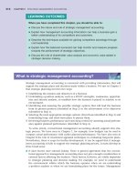
INTRODUCTION
3
When you have completed this chapter, you should be able to:
l Distinguish between fixed cost and variable cost and use this distinction to
explain the relationship between cost, volume and profit.
l Prepare a break-even chart and deduce the break-even point for some
activity.
l Discuss the weaknesses of break-even analysis.
l Demonstrate the way in which marginal analysis can be used when making
short-term decisions.
M03_ATRI3622_06_SE_C03.QXD 5/29/09 3:30 PM Page 55

We saw in the previous chapter that cost represents the resources that have to be
sacrificed to achieve a business objective. The objective may be to make a particular
product, to provide a particular service, to operate an IT department and so on. The
costs incurred by a business may be classified in various ways and one important way
is according to how they behave in relation to changes in the volume of activity. Costs
may be classified according to whether they
l remain constant (fixed) when changes occur to the volume of activity, or
l vary according to the volume of activity.
These are known as fixed cost and variable cost respectively. Thus, for example, in the

case of a restaurant, the manager’s salary would normally be a fixed cost while the
unprepared food would be a variable cost.
As we shall see, knowing how much of each type of cost is associated with a par-
ticular activity can be of great value to the decision maker.
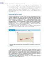
The way in which fixed cost behaves can be shown by preparing a graph that plots the
fixed cost of a business against the level of activity, as in Figure 3.1. The distance 0F
represents the amount of fixed cost, and this stays the same irrespective of the volume
of activity.
Fixed cost
Cost behaviour
CHAPTER 3 COST–VOLUME–PROFIT ANALYSIS
56
‘
Graph of fixed cost against the volume of activity
Figure 3.1
As the volume of output increases, the fixed cost stays exactly the same (0F).
M03_ATRI3622_06_SE_C03.QXD 5/29/09 3:30 PM Page 56

Staff salaries (or wages) are often assumed to be a variable cost but in practice they
tend to be fixed. Members of staff are not normally paid according to volume of out-
put and it is unusual to dismiss staff when there is a short-term downturn in activity.
Where there is a long-term downturn, or at least it seems that way to management,
redundancies may occur, with fixed-cost savings. This, however, is true of all types of
fixed cost. For example, management may also decide to close some branches to make
rental cost savings.
There are circumstances in which the labour cost is variable (for example, where staff
are paid according to how much output they produce), but this is unusual. Whether
labour cost is fixed or variable depends on the circumstances in the particular case
concerned.
It is important to be clear that ‘fixed’, in this context, means only that the cost is

unaffected by changes in the volume of activity. Fixed cost is likely to be affected by
inflation. If rent (a typical fixed cost) goes up because of inflation, a fixed cost will have
increased, but not because of a change in the volume of activity.
Similarly, the level of fixed cost does not stay the same irrespective of the time
period involved. Fixed cost elements are almost always time-based: that is, they vary
with the length of time concerned. The rental charge for two months is normally twice
that for one month. Thus, fixed cost normally varies with time, but (of course) not with
the volume of output. This means that when we talk of fixed cost being, say, £1,000,
we must add the period concerned, say, £1,000 a month.
FIXED COST
57
Can you give some examples of items of cost that are likely to be fixed for a hairdress-
ing business?
We came up with the following:
l rent
l insurance
l cleaning cost
l staff salaries.
These items of cost are likely to be the same irrespective of the number of customers hav-
ing their hair cut or styled.
Activity 3.1
Does fixed cost stay the same irrespective of the volume of output, even where there is
a massive rise in that volume? Think in terms of the rent cost for the hairdressing business.
In fact, the rent is only fixed over a particular range (known as the ‘relevant’ range). If the
number of people wanting to have their hair cut by the business increased, and the busi-
ness wished to meet this increased demand, it would eventually have to expand its phys-
ical size. This might be achieved by opening an additional branch, or perhaps by moving
the existing business to larger premises nearby. It may be possible to cope with relatively
minor increases in activity by using existing space more efficiently, or by having longer
opening hours. If activity continued to expand, however, increased rent charges would

seem inevitable.
Activity 3.2
M03_ATRI3622_06_SE_C03.QXD 5/29/09 3:30 PM Page 57

At lower volumes of activity, the rent cost shown in Figure 3.2 would be 0R. As the
volume of activity expands, the accommodation becomes inadequate and further
expansion requires an increase in premises and, therefore, cost. This higher level of
accommodation provision will enable further expansion to take place. Eventually,
additional cost will need to be incurred if further expansion is to occur. Elements of
fixed cost that behave in this way are often referred to as stepped fixed cost.
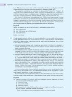
We saw earlier that variable cost varies with the volume of activity. In a manufactur-
ing business, for example, this would include the cost of raw materials used.
Variable cost can be represented graphically as in Figure 3.3. At zero volume of activ-
ity, the variable cost is zero. It then increases in a straight line as activity increases.
Variable cost
CHAPTER 3 COST–VOLUME–PROFIT ANALYSIS
58
‘
Graph of rent cost against the volume of activity
Figure 3.2
As the volume of activity increases from zero, the rent (a fixed cost) is unaffected. At a particu-
lar point, the volume of activity cannot increase further without additional space being rented.
The cost of renting the additional space will cause a ‘step’ in the rent cost. The higher rent cost
will continue unaffected if volume rises further until eventually another step point is reached.
Can you think of some examples of cost that are likely to be variable for a hairdressing
business?
We can think of a couple:
l lotions, sprays and other materials used;
l laundry cost to wash towels used to dry customers’ hair.
As with many types of business activity, variable cost incurred by hairdressers tends to be

low in comparison with fixed cost: that is, fixed cost tends to make up the bulk of total cost.
Activity 3.3
In practice, the situation described in Activity 3.2 would look something like Figure 3.2.
M03_ATRI3622_06_SE_C03.QXD 5/29/09 3:30 PM Page 58

The straight line for variable cost on Figure 3.3 implies that this type of cost will be
the same per unit of activity, irrespective of the volume of activity. We shall consider
the practicality of this assumption a little later in this chapter.
In some cases, cost has an element of both fixed and variable cost. It can then
be described as semi-fixed (semi-variable) cost. An example might be the electri-
city cost for the hairdressing business. Some of this will be for heating and lighting,
and this part is probably fixed, at least until the volume of activity expands to a
point where longer opening hours or larger premises are necessary. The other part
of the cost will vary with the volume of activity. An example would be power for
hairdryers.
Semi-fixed (semi-variable) cost
SEMI-FIXED (SEMI-VARIABLE) COST
59
‘
Graph of variable cost against the volume of activity
Figure 3.3
At zero activity, there is no variable cost. However, as the volume of activity increases, so does
the variable cost.
Can you suggest another cost for a hairdressing business that is likely to be semi-fixed
(semi-variable)?
We thought of telephone charges for landlines. These tend to have a rental element, which
is fixed, and there may also be certain calls that have to be made irrespective of the vol-
ume of activity involved. However, increased business would be likely to lead to the need
to make more telephone calls and so to increased call charges.
Activity 3.4

M03_ATRI3622_06_SE_C03.QXD 5/29/09 3:30 PM Page 59

From the graph we can say that the fixed element of the electricity cost is the
amount represented by the vertical distance from the origin at zero (bottom left-hand
corner) to the point where the line of best fit crosses the vertical axis of the graph. The
variable cost per unit is the amount that the graph rises for each increase in the vol-
ume of activity.
By breaking down semi-fixed cost into its fixed and variable elements in this way,
we are left with just two types of cost: fixed cost and variable cost.
Armed with knowledge of how much each element of cost represents for a particu-
lar product or service, it is possible to make predictions regarding total and per-unit
cost at various projected levels of output. Such predictive information can be very use-
ful to decision makers, and much of the rest of this chapter will be devoted to seeing
how, starting with break-even analysis.
Estimating semi-fixed (semi-variable) cost
Often, it is not obvious how much of each element a particular cost contains. However,
past experience may provide some guidance. Let us again take the example of electricity.
If we have data on what the electricity cost has been for various volumes of activity,
say the relevant data over several three-month periods (electricity is usually billed by
the quarter), we can estimate the fixed and variable portions. This may be done graphic-
ally, as shown in Figure 3.4. We tend to use past data here purely because they provide
us with an estimate of future cost; past cost is not, of course, relevant for its own sake.
Each of the dots in Figure 3.4 is the electricity charge for a particular quarter plotted
against the volume of activity (probably measured in terms of sales revenue) for the
same quarter. The diagonal line on the graph is the line of best fit. This means that this
was the line that best seemed (to us, at least) to represent the data. A better estimate
can usually be made using a statistical technique (least squares regression), which does
not involve drawing graphs and making estimates. In practice, though, it probably
makes little difference which approach is taken.
CHAPTER 3 COST–VOLUME–PROFIT ANALYSIS

60
‘
Graph of electricity cost against the volume of activity
Figure 3.4
Here the electricity bill for a time period (for example, three months) is plotted against the vol-
ume of activity for that same period. This is done for a series of periods. A line is then drawn
that best ‘fits’ the various points on the graph. From this line we can then deduce both the cost
at zero activity (the fixed element) and the slope of the line (the variable element).
M03_ATRI3622_06_SE_C03.QXD 5/29/09 3:30 PM Page 60

If, for a particular product or service, we know the fixed cost for a period and the vari-
able cost per unit, we can produce a graph like the one shown in Figure 3.5. This graph
reveals the total cost over the possible range of volume of activity.
Finding the break-even point
The bottom part of Figure 3.5 shows the fixed-cost area. Added to this is the variable
cost, the wedge-shaped portion at the top of the graph. The uppermost line represents
the total cost over a range of volume of activity. For any particular volume, the total
cost can be measured by the vertical distance between the graph’s horizontal axis and
the relevant point on the uppermost line.
Logically, the total cost at zero activity is the amount of the fixed cost. This is
because, even where there is nothing going on, the business will still be paying rent,
salaries and so on, at least in the short term. As the volume of activity increases from
zero, the fixed cost is augmented by the relevant variable cost to give the total cost.
If we take this total cost graph in Figure 3.5, and superimpose on it a line represent-
ing total revenue over the range of volume of activity, we obtain the break-even chart.
This is shown in Figure 3.6.
Note in Figure 3.6 that, at zero volume of activity (zero sales), there is zero sales rev-
enue. The profit (loss), which is the difference between total sales revenue and total
cost, for a particular volume of activity is the vertical distance between the total sales
revenue line and the total cost line at that volume of activity. Where there is no ver-

tical distance between these two lines (total sales revenue equals total cost) the volume
of activity is at break-even point (BEP). At this point there is neither profit nor loss:
that is, the activity breaks even. Where the volume of activity is below BEP, a loss will
be incurred because total cost exceeds total sales revenue. Where the business operates
at a volume of activity above BEP, there will be a profit because total sales revenue will
FINDING THE BREAK-EVEN POINT
61
‘
‘
Graph of total cost against volume of activity
Figure 3.5
The bottom part of the graph represents the fixed cost element. To this is added the wedge-
shaped top portion, which represents the variable cost. The two parts together represent total
cost. At zero activity, the variable cost is zero, so total cost equals fixed cost. As activity
increases so does total cost, but only because variable cost increases. We are assuming that
there are no steps in the fixed cost.
M03_ATRI3622_06_SE_C03.QXD 5/29/09 3:30 PM Page 61

exceed total cost. The further below BEP, the higher the loss; the further above BEP, the
higher the profit.
Deducing BEPs by graphical means is a laborious business. Since, however, the
relationships in the graph are all linear (that is, the lines are all straight), it is easy to
calculate the BEP.
We know that at BEP (but not at any other point)
Total sales revenue
==
Total cost
(At all other points except the BEP, either total sales revenue will exceed total cost or
the other way round. Only at BEP are they equal.) The above formula can be expanded
so that

Total sales revenue
==
Fixed cost
++
Total variable cost
If we call the number of units of output at BEP b, then
b × Sales revenue per unit = Fixed cost + (b × Variable cost per unit)
so
(b × Sales revenue per unit) − (b × Variable cost per unit) = Fixed cost
and
b × (Sales revenue per unit − Variable cost per unit) = Fixed cost
giving
b
==
Fixed cost
Sales revenue per unit
−−
Variable costs per unit
CHAPTER 3 COST–VOLUME–PROFIT ANALYSIS
62
Break-even chart
Figure 3.6
The sloping line starting at zero represents the sales revenue at various volumes of activity. The
point at which this finally catches up with the sloping total cost line, which starts at F, is the
break-even point (BEP). Below this point a loss is made, above it a profit.
M03_ATRI3622_06_SE_C03.QXD 5/29/09 3:30 PM Page 62

If we look back at the break-even chart in Figure 3.6, this formula seems logical. The
total cost line starts off at point F, higher than the starting point for the total sales rev-
enues line (zero) by amount F (the amount of the fixed cost). Because the sales revenue

per unit is greater than the variable cost per unit, the sales revenue line will gradually
catch up with the total cost line. The rate at which it will catch up is dependent on the
relative steepness of the two lines and the amount that it has to catch up (the fixed
cost). Bearing in mind that the slopes of the two lines are the variable cost per unit and
the selling price per unit, the above equation for calculating b looks perfectly logical.
Though the BEP can be calculated quickly and simply without resorting to graphs,
this does not mean that the break-even chart is without value. The chart shows the
relationship between cost, volume and profit over a range of activity and in a form that
can easily be understood by non-financial managers. The break-even chart can there-
fore be a useful device for explaining this relationship.
Real World 3.1 shows information on the BEPs of three well-known businesses.
FINDING THE BREAK-EVEN POINT
63
Cottage Industries Ltd makes baskets. The fixed costs of operating the workshop
for a month total £500. Each basket requires materials that cost £2. Each basket
takes one hour to make, and the business pays the basket makers £10 an hour.
The basket makers are all on contracts such that if they do not work for any rea-
son, they are not paid. The baskets are sold to a wholesaler for £14 each.
What is the BEP for basket making for the business?
Solution
The BEP (in number of baskets)
=
=
= 250 baskets per month
Note that the BEP must be expressed with respect to a period of time.
£500
£14 − (£2 + £10)
Fixed cost
(Sales revenue per unit − Variable cost per unit)
Example 3.1

REAL WORLD 3.1
BE at BA, Ryanair and easyJet
Commercial airlines seem to pay a lot of attention to their BEPs and their ‘load factors’,
that is, their actual level of activity. Figure 3.7 shows the BEP and load factor for three well-
known airlines operating from the UK. British Airways (BA) is a traditional airline. Ryanair
and easyJet are both ‘no-frills’ carriers, which means that passengers receive lower levels
of service in return for lower fares. All three operate flights within the UK and from the UK
‘
M03_ATRI3622_06_SE_C03.QXD 5/29/09 3:30 PM Page 63

CHAPTER 3 COST–VOLUME–PROFIT ANALYSIS
64
Can you think of reasons why the managers of a business might find it useful to know
the BEP of some activity that they are planning to undertake?
By knowing the BEP, it is possible to compare the expected, or planned, volume of activ-
ity with the BEP and so make a judgement about risk. If the volume of activity is expected
to only just exceed the break-even point, this may suggest that it is a risky venture. Only
a small fall from the expected volume of activity could lead to a loss.
Activity 3.5
Cottage Industries Ltd (see Example 3.1) expects to sell 500 baskets a month. The
business has the opportunity to rent a basket-making machine. Doing so would
increase the total fixed cost of operating the workshop for a month to £3,000. Using the
machine would reduce the labour time to half an hour per basket. The basket makers
would still be paid £10 an hour.
Activity 3.6
Real World 3.1 continued
Source: Based on information contained in Binggeli, U. and Pompeo, L., ‘The battle for Europe’s low-fare flyers’, The McKinsey
Quarterly, August 2005 (www.mckinseyquarterly.com). The data in the article are based on the year ended 31 March 2004.
to other countries. BA offers a much wider range of destinations than the other two air-
lines. We can see that all three airlines were making operating profits as each had a load

factor greater than its BEP.
Break-even and load factors in the airline industry
Figure 3.7
M03_ATRI3622_06_SE_C03.QXD 5/29/09 3:30 PM Page 64

In the same way as we can derive the number of units of output necessary to break
even, we can calculate the volume of activity required to achieve a particular level of
profit. We can expand the equation shown on p. 62 above so that
Total sales revenue
==
Fixed cost
++
Total variable cost
++
Target profit
Achieving a target profit
ACHIEVING A TARGET PROFIT
65
(a) How much profit would the business make each month from selling baskets
1 assuming that the basket-making machine is not rented; and
2 assuming that it is rented?
(b) What is the BEP if the machine is rented?
(c) What do you notice about the figures that you calculate?
(a) Estimated monthly profit from basket making:
Without the machine With the machine
££££
Sales revenue (500 × £14) 7,000 7,000
Materials (500 × £2) (1,000) (1,000)
Labour (500 × 1 × £10) (5,000)
(500 ×

1
/2 × £10) (2,500)
Fixed cost (500 ) (3,000)
( 6,500 ) (6,500 )
Profit 500 500
(b) The BEP (in number of baskets) with the machine
=
=
= 429 baskets a month
The BEP without the machine is 250 baskets per month (see Example 3.1).
(c) There seems to be nothing to choose between the two manufacturing strategies
regarding profit, at the estimated sales volume. There is, however, a distinct difference
between the two strategies regarding the BEP. Without the machine, the actual vol-
ume of sales could fall by a half of that which is expected (from 500 to 250) before the
business would fail to make a profit. With the machine, however, just a 14 per cent fall
(from 500 to 429) would be enough to cause the business to fail to make a profit. On
the other hand, for each additional basket sold above the estimated 500, an additional
profit of only £2 (that is, £14 − (£2 + £10)) would be made without the machine,
whereas £7 (that is, £14 − (£2 + £5)) would be made with the machine. (Note that
knowledge of the BEP and the planned volume of activity gives some basis for
assessing the riskiness of the activity.)
£3,000
£14 − (£2 + £5)
Fixed cost
Sales revenue per unit − Variable cost per unit
M03_ATRI3622_06_SE_C03.QXD 5/29/09 3:30 PM Page 65

If we let t be the required number of units of output to achieve the target profit, then
t × Sales revenue per unit = Fixed cost + (t × Variable cost per unit) + Target profit
so

(t × Sales revenue per unit) − (t × Variable cost per unit) = Fixed cost + Target profit
and
t × (Sales revenue per unit − Variable cost per unit) = Fixed cost + Target profit
giving
t
==
Fixed cost
++
Target profit
(Sales revenue per unit
−−
Variable cost per unit)
We shall take a closer look at the relationship between fixed cost, variable cost and
profit together with any advice that we might give the management of Cottage Industries
Ltd after we have briefly considered the notion of contribution.
The bottom part of the break-even formula (sales revenue per unit less variable cost
per unit) is known as the contribution per unit. Thus for the basket-making activity,
without the machine the contribution per unit is £2, and with the machine it is £7.
This can be quite a useful figure to know in a decision-making context. It is called
‘contribution’ because it contributes to meeting the fixed cost and, if there is any
excess, it then contributes to profit.
We shall see, a little later in this chapter, how knowing the amount of the contri-
bution generated by a particular activity can be valuable in making short-term deci-
sions of various types, as well as being useful in the BEP calculation.
Contribution
CHAPTER 3 COST–VOLUME–PROFIT ANALYSIS
66
‘
What volume of activity is required by Cottage Industries Ltd (see Example 3.1 and
Activity 3.6) in order to make a profit of £4,000 a month

(a) assuming that the basket-making machine is not rented; and
(b) assuming that it is rented?
(a) Using the formula above, the required volume of activity without the machine is
==2,250 baskets a month
(b) The required volume of activity with the machine is
==1,000 baskets a month
£3,000 + £4,000
£14 − (£2 + £5)
£500 + £4,000
£14 − (£2 + £10)
Fixed cost + Target profit
(Sales revenue per unit − Variable cost per unit)
Activity 3.7
M03_ATRI3622_06_SE_C03.QXD 5/29/09 3:30 PM Page 66

The relative margins of safety are directly linked to the relationship between the sell-
ing price per basket, the variable cost per basket and the fixed cost per month. Without
the machine the contribution (selling price less variable cost) per basket is £2; with the
machine it is £7. On the other hand, without the machine the fixed cost is £500 a
month; with the machine it is £3,000. This means that, with the machine, the contri-
butions have more fixed cost to ‘overcome’ before the activity becomes profitable.
Contribution margin ratio
The contribution margin ratio is the contribution from an activity expressed as a per-
centage of the sales revenue, thus:
Contribution margin ratio
== ××
100%
Contribution and sales revenue can both be expressed in per-unit or total terms.
For Cottage Industries Ltd (see Example 3.1 and Activity 3.6), the contribution margin
ratios are:

l without the machine, × 100% = 14%
l with the machine, × 100% = 50%
The ratio can provide an impression of the extent to which sales revenue is eaten
away by variable cost.
The margin of safety is the extent to which the planned volume of output or sales lies
above the BEP. Going back to Activity 3.6, we saw that the following situation exists:
Without the machine With the machine
(number of baskets) (number of baskets)
Expected volume of sales 500 500
BEP 250 429
Difference (margin of safety):
Number of baskets 250 71
Percentage of estimated volume of sales 50% 14%
Margin of safety
14 − 7
14
14 − 12
14
Contribution
Sales revenue
MARGIN OF SAFETY
67
‘
‘
What advice would you give Cottage Industries Ltd about renting the machine, on the
basis of the values for margin of safety?
It is a matter of personal judgement, which in turn is related to individual attitudes to risk,
as to which strategy to adopt. Most people, however, would prefer the strategy of not rent-
ing the machine, since the margin of safety between the expected volume of activity and
the BEP is much greater. Thus, for the same level of return, the risk will be lower without

renting the machine.
Activity 3.8
M03_ATRI3622_06_SE_C03.QXD 5/29/09 3:30 PM Page 67

However, the rate at which the contributions can overcome fixed cost is higher with
the machine, because variable cost is lower. Thus, one more, or one less, basket sold
has a greater impact on profit than it does if the machine is not rented. The contrast
between the two scenarios is shown graphically in Figures 3.8(a) and 3.8(b).
CHAPTER 3 COST–VOLUME–PROFIT ANALYSIS
68
Break-even charts for Cottage Industries’ basket-making
activities (a) without the machine and (b) with the machine
Figure 3.8
Without the machine the contribution per basket is low. Thus, each additional basket sold does not
make a dramatic difference to the profit or loss. With the machine, however, the opposite is true,
and small increases or decreases in the sales volume will have a great effect on the profit or loss.
M03_ATRI3622_06_SE_C03.QXD 5/29/09 3:30 PM Page 68

If we look back to Real World 3.1 (page 63), we can see that Ryanair had a much
larger margin of safety than either BA or easyJet.
Real World 3.2 goes into more detail on the margin of safety and operating profit,
over recent years, of one of the three airlines featured in Real World 3.1.
MARGIN OF SAFETY
69
REAL WORLD 3.2
BA’s margin of safety
As we saw in Real World 3.1, commercial airlines pay a lot of attention to BEPs. They are
also interested in their margin of safety (the difference between load factor and BEP).
Figure 3.9 shows BA’s margin of safety and its operating profit over a seven-year
period. Note that in 2002, BA had a load factor that was below its break-even point and

this caused an operating loss. In the other years, the load factors were comfortably greater
than the BEP. This led to operating profits.
Source: British Airways plc Annual Reports 2002 to 2008.
BA’s margin of safety
Figure 3.9
The margin of safety is expressed as the difference between the load factor and the BEP
(for each year), expressed as a percentage of the BEP. Generally, the higher the margin
of safety, the higher the operating profit.
M03_ATRI3622_06_SE_C03.QXD 5/29/09 3:30 PM Page 69

The relationship between contribution and fixed cost is known as operating gearing
(or operational gearing). An activity with a relatively high fixed cost compared with its
variable cost is said to have high operating gearing. Thus, Cottage Industries Ltd has
higher operating gearing using the machine than it has if not using it. Renting the
machine increases the level of operating gearing quite dramatically because it causes
an increase in fixed cost, but at the same time it leads to a reduction in variable cost
per basket.
The effect of gearing on profit
The reason why the word ‘gearing’ is used in this context is that, as with intermeshing
gear wheels of different circumferences, a circular movement in one of the factors (vol-
ume of output) causes a more-than-proportionate circular movement in the other
(profit) as illustrated by Figure 3.10.
Operating gearing
CHAPTER 3 COST–VOLUME–PROFIT ANALYSIS
70
‘
‘
The effect of operating gearing
Figure 3.10
Where operating gearing is relatively high, as in the diagram, a small amount of circular motion

in the volume wheel causes a relatively large amount of circular motion in the profit wheel. An
increase in volume would cause a disproportionately greater increase in profit. The equivalent
would also be true of a decrease in activity, however.
M03_ATRI3622_06_SE_C03.QXD 5/29/09 3:30 PM Page 70

Increasing the level of operating gearing makes profits more sensitive to changes in
the volume of activity. We can demonstrate operating gearing with Cottage Industries
Ltd’s basket-making activities as follows:
Without the machine With the machine
Volume (number 500 1,000 1,500 500 1,000 1,500
of baskets)
££££££
Contribution* 1,000 2,000 3,000 3,500 7,000 10,500
Fixed cost (500 ) (500 ) (500 ) ( 3,000 ) ( 3,000 ) (3,000 )
Profit 500 1,500 2,500 500 4,000 7,500
* £2 per basket without the machine and £7 per basket with it.
Note that, without the machine (low operating gearing), a doubling of the output
from 500 to 1,000 units brings a trebling of the profit. With the machine (high oper-
ating gearing), doubling output causes profit to rise by eight times. At the same time,
reductions in the volume of output tend to have a more damaging effect on profit
where the operating gearing is higher.
Real World 3.3 shows how a very well-known business has benefited from high oper-
ating gearing.
OPERATING GEARING
71
Generally speaking, what types of business activity are likely to have high operating
gearing? (Hint: Cottage Industries Ltd might give you some idea.)
Activities that are capital-intensive tend to have high operating gearing This is because
renting or owning capital equipment gives rise to additional fixed cost, but it can also give
rise to lower variable cost.

Activity 3.9
REAL WORLD 3.3
Check out operating gearing
After several years of disappointing trading and loss of market share, in 2004, the UK
supermarket company J Sainsbury plc set a plan to improve its profitability and gain mar-
ket share. During the period from 2005 to 2008, Sainsbury’s increased its sales revenue
by 16 per cent, but this fed through to a 105 per cent increase in profit. This was partly
due to relatively high operating gearing, which caused the profit to increase at a much
greater rate than the sales revenue. Quite a lot of retailers’ costs are fixed – rent, salaries,
heat and light, training and advertising for example.
In its 2008 annual report Sainsbury’s Chief Executive, Justin King, said ‘Our sales
growth is reflected in substantially improved profits and operational gearing is coming
through.’
Source: J Sainsbury plc Annual Report 2008, page 4.
M03_ATRI3622_06_SE_C03.QXD 5/29/09 3:30 PM Page 71

A slight variant of the break-even chart is the profit–volume (PV) chart. A typical PV
chart is shown in Figure 3.11.
Profit–volume charts
The profit–volume chart is obtained by plotting loss or profit against volume of
activity. The slope of the graph is equal to the contribution per unit, since each addi-
tional unit sold decreases the loss, or increases the profit, by the sales revenue per unit
less the variable cost per unit. At zero volume of activity there are no contributions, so
there is a loss equal to the amount of the fixed cost. As the volume of activity increases,
the amount of the loss gradually decreases until BEP is reached. Beyond BEP a profit is
made, which increases as activity increases.
As we can see, the profit–volume chart does not tell us anything not shown by the
break-even chart. It does, however, highlight key information concerning the profit
(loss) arising at any volume of activity. The break-even chart shows this as the vertical
distance between the total cost and total sales revenue lines. The profit–volume chart,

in effect, combines the total sales revenue and total variable cost lines, which means
that profit (or loss) is directly readable.
So far in this chapter we have treated all the relationships as linear – that is, all of the
lines in the graphs have been straight. This is typically the approach taken in manage-
ment accounting, though it may not be strictly valid.
Consider, for example, the variable cost line in the break-even chart; accountants
would normally treat this as being a straight line. Strictly, however, the line should
The economist’s view of the break-even chart
CHAPTER 3 COST–VOLUME–PROFIT ANALYSIS
72
‘
Profit–volume chart
Figure 3.11
The sloping line is profit (loss) plotted against activity. As activity increases, so does total con-
tribution (sales revenue less variable cost). At zero activity there are no contributions, so there
will be a loss equal in amount to the total fixed cost.
M03_ATRI3622_06_SE_C03.QXD 5/29/09 3:30 PM Page 72

probably not be straight because at high levels of output economies of scale may be
available to an extent not available at lower levels. For example, a raw material (a typ-
ical variable cost) may be able to be used more efficiently with higher volumes of activ-
ity. Similarly, buying large quantities of material and services may enable the business
to benefit from bulk discounts and so lower its costs.
There is also a tendency for sales revenue per unit to reduce as volume is increased.
To sell more of a particular product or service, it will usually be necessary to lower the
price per unit.
Economists recognise that, in real life, the relationships portrayed in the break-even
chart are usually non-linear. The typical economist’s view of the chart is shown in
Figure 3.12.
Note, in Figure 3.12, that the total variable cost line starts to rise quite steeply with

volume but, around point A, economies of scale start to take effect. With further
increases in volume, total variable cost does not rise as steeply because variable cost for
each additional unit of output is lowered. These economies of scale continue to have a
benign effect on cost until a point is reached where the business is operating towards
the end of its efficient range. Beyond this range, problems will emerge that adversely
affect variable cost. For example, the business may be unable to find cheap supplies of
the variable-cost elements, or may suffer production difficulties such as machine break-
downs. As a result, the total variable cost line starts to rise more steeply
At low levels of output, sales may be made at a relatively high price per unit. To
increase sales output beyond point B, however, it may be necessary to lower the aver-
age sales price per unit. This will mean that the total revenue line will not rise as
steeply, and may even curve downwards.
Note how this ‘curvilinear’ representation of the break-even chart can easily lead to
the existence of two break-even points.
THE ECONOMIST’S VIEW OF THE BREAK-EVEN CHART
73
‘
The economist’s view of the break-even chart
Figure 3.12
As volume increases, economies of scale have a favourable effect on variable cost, but this
effect is reversed at still higher levels of output. At the same time, sales revenue per unit will
tend to decrease at higher levels to encourage additional buyers.
M03_ATRI3622_06_SE_C03.QXD 5/29/09 3:30 PM Page 73

Accountants justify their approach to this topic by the fact that, though the lines
may not, in practice, be perfectly straight, this defect is probably not worth taking
into account in most cases. This is partly because all of the information used in the
analysis is based on estimates of the future. As this will inevitably be flawed, it seems
pointless to be pedantic about minor approximations, such as treating the total cost
and total revenue lines as straight when strictly this is not so. Only where significant

economies or diseconomies of scale are involved should the non-linearity of the vari-
able cost be taken into account. Also, for most businesses, the range of possible vol-
umes of activity at which they are capable of operating (the relevant range) is pretty
narrow. Over very short distances, it is perfectly reasonable to treat a curved line as
being straight.
Where a business fails to reach its BEP, steps must be taken to remedy the problem:
there must be an increase in sales revenue or a reduction in cost, or both of these.
Real World 3.4 reveals that Ford’s subsidiary Volvo is struggling to reach its BEP. Ford
has recently disposed of its three UK luxury brands (Aston Martin, Jaguar and Land
Rover) and is thought to be considering the possibility of selling off Volvo as well.
Failing to break even
As we have seen, break-even analysis can provide some useful insights concerning the
important relationship between fixed cost, variable cost and the volume of activity. It
does, however, have its weaknesses. There are three general problems:
l Non-linear relationships. The management accountant’s normal approach to break-
even analysis assumes that the relationships between sales revenues, variable cost
Weaknesses of break-even analysis
CHAPTER 3 COST–VOLUME–PROFIT ANALYSIS
74
‘
REAL WORLD 3.4
Trying to keep on the road
Volvo Cars said on Wednesday it was cutting about 8 per cent of its global staff in response to
soaring raw material costs and weaker sales on the US and European markets.
The axing of 2,000 jobs is the largest in the history of the premium brand, owned by Ford Motor,
and created a stir in Sweden, where other exporters have also been hurt by the weak dollar.
Volvo reported a net loss of $151m in the first quarter of this year, compared with a profit of
$94m a year ago.
Volvo has been hit harder than most other carmakers by the weakening of the dollar because
it produces no cars in the US, unlike Japanese and Korean manufacturers or Germany’s BMW and

Mercedes-Benz brands. The brand sold 458,000 cars worldwide last year and the US is its largest
market.
The pain at Volvo adds to mounting problems at Ford, which has abandoned pledges to break
even next year and return to profit in 2010 due to a sharp contraction in US sales of its profitable
large pick-ups and sport utility vehicles.
Source: Extracts from Reed, J. and Anderson, R., ‘Volvo to cut 8 per cent of global staff’, ft.com, 25 June 2008.
FT
M03_ATRI3622_06_SE_C03.QXD 5/29/09 3:30 PM Page 74

and volume are strictly straight-line ones. In real life, this is unlikely to be the case.
This is probably not a major problem, since, as we have just seen,
– break-even analysis is normally conducted in advance of the activity actually
taking place. Our ability to predict future cost, revenue and so on is somewhat
limited, so what are probably minor variations from strict linearity are unlikely to
be significant, compared with other forecasting errors; and
– most businesses operate within a narrow range of volume of activity; over short
ranges, curved lines tend to be relatively straight.
l Stepped fixed cost. Most types of fixed cost are not fixed over all volumes of activity.
They tend to be ‘stepped’ in the way depicted in Figure 3.2. This means that, in prac-
tice, great care must be taken in making assumptions about fixed cost. The problem
is heightened because most activities will probably involve various types of fixed
cost (for example rent, supervisory salaries, administration costs), all of which are
likely to have steps at different points.
l Multi-product businesses. Most businesses do not offer just one product or service.
This is a problem for break-even analysis since it raises the question of the effect of
additional sales of one product or service on sales of another of the business’s pro-
ducts or services. There is also the problem of identifying the fixed cost of one
particular activity. Fixed cost tends to relate to more than one activity – for example,
two activities may be carried out in the same rented premises. There are ways of
dividing the fixed cost between activities, but these tend to be arbitrary, which calls

into question the value of the break-even analysis and any conclusions reached.
WEAKNESSES OF BREAK-EVEN ANALYSIS
75
We saw above that, in practice, relationships between costs, revenues and volumes of
activity are not necessarily straight-line ones.
Can you think of at least three reasons, with examples, why that may be the case?
We thought of the following:
l Economies of scale with labour. A business may do things more economically where
there is a high volume of activity than is possible at lower levels of activity. It may, for
example, be possible for employees to specialise.
l Economies of scale with buying goods or services. A business may find it cheaper to
buy in goods and services where it is buying in bulk, as discounts are often given.
l Diseconomies of scale. This may mean that the per-unit cost of output is higher at
higher levels of activity. For example, it may be necessary to pay higher rates of pay to
workers to recruit the additional staff needed at higher volumes of activity.
l Lower sales prices at high levels of activity. Some consumers may only be prepared to
buy the particular product or service at a lower price. Thus, it may not be possible
to achieve high levels of sales activity without lowering the selling price.
Activity 3.10
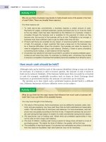
Despite some practical problems, break-even analysis and BEP seem to be widely
used. The media frequently refer to the BEP for businesses and activities. For example,
there is seemingly constant discussion about Eurotunnel’s BEP and whether it will
ever be reached. Similarly, the number of people regularly needed to pay to watch a
football team so that the club breaks even is often mentioned. This is illustrated in
Real World 3.5, which is an extract from an article discussing the failure of Plymouth
Argyle FC, the Coca-Cola Championship football club, to spend all of its player trans-
fer income on new players.
M03_ATRI3622_06_SE_C03.QXD 5/29/09 3:30 PM Page 75

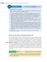
Real World 3.7 provides a more formal insight into the extent to which managers in

practice use break-even analysis.
CHAPTER 3 COST–VOLUME–PROFIT ANALYSIS
76
REAL WORLD 3.5
Pilgrims not progressing through the turnstiles
This year, Argyle have raked in plenty of income, in addition to their gate receipts. The sale of
players has brought in over £8 million. Their expenditure has been nowhere near that sum.
The failure to sign adequate replacements for the departed players could put Argyle’s
Championship status in jeopardy. Yes, the Pilgrims have to retain some of their transfer
income to help them cope with running costs – they do not break even on current gates –
but the best way to increase attendances is to provide an attractive and successful team.
Source: Metcalf, R., ‘Argyle viewpoint’, Western Morning News, 15 September 2008.
REAL WORLD 3.6
Breaking even is breaking out all over
Setanta sets its break-even target
Setanta Sports Holdings Ltd, the satellite TV broadcaster and rival of BSkyB, has a break-
even point of about 1.5 million subscribers. By April 2009, Setanta plans to have 4 million
subscribers.
Source: Fenton, B., ‘Setanta chases fresh targets’, Financial Times, 23 July 2008.
Superjumbo break-even point grows
German industrial group EADS is developing the Airbus A380 aircraft. The aircraft can
carry up to 555 passengers on each flight. When EADS approved development of the
plane in 2000, it was estimated that the business would need to sell 250 of them to break
even. By 2005, the break-even number had increased to 270, but by early 2008 the cost
of development had increased to the point where it was estimated that it would require
sales of 400 of the aircraft for it to break even. Expected total sales of the aircraft could
be about 1,000 over its commercial lifetime.
Source: ‘EADS and the A380’, Financial Times, 27 February 2008.
City Link to break even
City Link, the parcel delivery business owned by Rentokil Initial plc, was expected only to

break even in 2008. This was as a result of inadequate management information systems,
which led to loss of customers.
Source: Davoudi, S. and Urry, M., ‘Rentokil plunge spurs break-up fears’, Financial Times, 28 February 2008.
Real World 3.6 shows specific references to break-even point for three well-known
businesses.
FT
M03_ATRI3622_06_SE_C03.QXD 5/29/09 3:30 PM Page 76