Monetary and Fiscal Strategies in the World Economy by Michael Carlberg_6 pdf

187
Then the first-order condition for a minimum loss gives the reaction function of
the American central bank:


222 211
2M A B 2G G M=−− −+ (12)

Suppose the European central bank lowers European money supply. Then, as a
response, the American central bank lowers American money supply.

The targets of the European government are zero unemployment and a zero
structural deficit in Europe. The instrument of the European government is
European government purchases. There are two targets but only one instrument,
so what is needed is a loss function. We assume that the European government
has a quadratic loss function:


22
111
LG u s=+
(13)

1
LG is the loss to the European government caused by unemployment and the
structural deficit in Europe. We assume equal weights in the loss function. The
specific target of the European government is to minimize its loss, given the
unemployment function and the structural deficit function. Taking account of
equations (1) and (5), the loss function of the European government can be
written as follows:

22
111 21 2 11
LG (A M 0.5M G 0.5G ) (G T )=−+ −− +−
(14)

Then the first-order condition for a minimum loss gives the reaction function of
the European government:


111122
4G 2A 2T 2M M G=+−+− (15)

The targets of the American government are zero unemployment and a zero
structural deficit in America. The instrument of the American government is
American government purchases. There are two targets but only one instrument,
so what is needed is a loss function. We assume that the American government
has a quadratic loss function:

1. The Model

188

22
222
LG u s=+
(16)

2

LG is the loss to the American government caused by unemployment and the
structural deficit in America. We assume equal weights in the loss function. The
specific target of the American government is to minimize its loss, given the
unemployment function and the structural deficit function. Taking account of
equations (2) and (6), the loss function of the American government can be
written as follows:


22
222 12 1 22
LG (A M 0.5M G 0.5G ) (G T )=−+ −− +−
(17)

Then the first-order condition for a minimum loss gives the reaction function of
the American government:


222211
4G 2A 2T 2M M G=+−+− (18)

Suppose the European government raises European government purchases. Then,
as a response, the European central bank lowers European money supply, the
American central bank lowers American money supply, and the American
government lowers American government purchases.

The Nash equilibrium is determined by the reaction functions of the
European central bank, the American central bank, the European government,
and the American government. We assume
12
TT T

=
= . The solution to this
problem is as follows:


11212
6M A 2A 9B 6B 18T=− − − − − (19)

22121
6M A 2A 9B 6B 18T=− − − − − (20)

111
2G A B 2T=++ (21)

222
2G A B 2T=++ (22)

Equations (19) to (22) show the Nash equilibrium of European money supply,
American money supply, European government purchases, and American
government purchases. As a result there is a unique Nash equilibrium. An
increase in
1
A causes a decline in European money supply, a decline in
Monetary and Fiscal Interaction between Europe and America: Case B

189
American money supply, an increase in European government purchases, and no
change in American government purchases. A unit increase in
1
A causes a

decline in European money supply of 0.17 units, a decline in American money
supply of 0.33 units, and an increase in European government purchases of 0.5
units.




2. Some Numerical Examples



For easy reference, the basic model is reproduced here:


111 21 2
uAM0.5MG0.5G=− + −− (1)

222 12 1
uAM0.5MG0.5G=− + −− (2)

11 1 21 2
B M 0.5M G 0.5Gπ= + − + + (3)

22 2 12 1
B M 0.5M G 0.5Gπ= + − + + (4)

111
sGT=− (5)

222

sGT=− (6)

And the Nash equilibrium can be described by four equations:


11212
6M A 2A 9B 6B 18T=− − − − − (7)

22121
6M A 2A 9B 6B 18T=− − − − − (8)

111
2G A B 2T=++ (9)

222
2G A B 2T=++ (10)

It proves useful to study eight distinct cases:
-
a demand shock in Europe
-
a supply shock in Europe
-
a mixed shock in Europe
2. Some Numerical Examples

190
- another mixed shock in Europe
-
a common demand shock

-
a common supply shock
-
a common mixed shock
-
another common mixed shock.

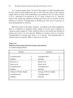
1) A demand shock in Europe. In each of the regions, let initial
unemployment be zero, let initial inflation be zero, and let the initial structural
deficit be zero as well. Step one refers to a decline in the demand for European
goods. In terms of the model there is an increase in
1
A of 3 units and a decline in
1
B of equally 3 units. Step two refers to the outside lag. Unemployment in
Europe goes from zero to 3 percent. Unemployment in America stays at zero
percent. Inflation in Europe goes from zero to – 3 percent. Inflation in America
stays at zero percent. The structural deficit in Europe stays at zero percent, as
does the structural deficit in America.

Step three refers to the policy response. According to the Nash equilibrium
there is an increase in European money supply of 4 units, an increase in
American money supply of 2 units, no change in European government
purchases, and no change in American government purchases. Step four refers to
the outside lag. Unemployment in Europe goes from 3 to zero percent.
Unemployment in America stays at zero percent. Inflation in Europe goes from
– 3 to zero percent. Inflation in America stays at zero percent. The structural
deficit in Europe stays at zero percent, as does the structural deficit in America.
For a synopsis see Table 7.7.

As a result, given a demand shock in Europe, monetary and fiscal interaction
produces zero inflation, zero unemployment, and a zero structural deficit in each
of the regions.

The loss functions of the European central bank, the American central bank,
the European government, and the American government are respectively:


22
111
LM u=π +
(11)

22
222
LM u=π +
(12)

22
111
LG u s=+
(13)
Monetary and Fiscal Interaction between Europe and America: Case B

191

22
222
LG u s=+
(14)

The initial loss of each policy maker is zero. The demand shock in Europe causes
a loss to the European central bank of 18 units, a loss to the European
government of 9 units, a loss to the American central bank of zero, and a loss to
the American government of zero. Then policy interaction reduces the loss of the
European central bank from 18 to zero units. Correspondingly, it reduces the loss
of the European government from 9 to zero units. Policy interaction keeps the
loss of the American central bank at zero. Similarly, it keeps the loss of the
American government at zero.


Table 7.7
Monetary and Fiscal Interaction between Europe and America
A Demand Shock in Europe

Europe America

Unemployment 0 Unemployment 0
Inflation 0 Inflation 0
Structural Deficit 0 Structural Deficit 0
Shock in A
1

3
Shock in B
1

− 3

Unemployment 3 Unemployment 0

Inflation
− 3
Inflation 0
Change in Money Supply 4 Change in Money Supply 2
Change in Govt Purchases 0 Change in Govt Purchases 0
Unemployment 0 Unemployment 0
Inflation 0 Inflation 0
Structural Deficit 0 Structural Deficit 0



2. Some Numerical Examples

192
2) A supply shock in Europe. In each of the regions let initial unemployment
be zero, let initial inflation be zero, and let the initial structural deficit be zero as
well. Step one refers to the supply shock in Europe. In terms of the model there is
an increase in
1
B of 3 units and an increase in
1
A of equally 3 units. Step two
refers to the outside lag. Inflation in Europe goes from zero to 3 percent. Inflation
in America stays at zero percent. Unemployment in Europe goes from zero to 3
percent. And unemployment in America stays at zero percent.

Step three refers to the policy response. According to the Nash equilibrium
there is a reduction in European money supply of 5 units, a reduction in
American money supply of 4 units, an increase in European government
purchases of 3 units, and no change in American government purchases. Step

four refers to the outside lag. Inflation in Europe stays at 3 percent. Inflation in
America stays at zero percent. Unemployment in Europe stays at 3 percent.
Unemployment in America stays at zero percent. The structural deficit in Europe
goes from zero to 3 percent. And the structural deficit in America stays at zero
percent. For an overview see Table 7.8.

First consider the effects on Europe. As a result, given a supply shock in
Europe, monetary and fiscal interaction has no effects on inflation and
unemployment in Europe. And what is more, it causes a structural deficit there.
Second consider the effects on America. As a result, monetary and fiscal
interaction produces zero inflation, zero unemployment, and a zero structural
deficit in America.

The initial loss of each policy maker is zero. The supply shock in Europe
causes a loss to the European central bank of 18 units, a loss to the European
government of 9 units, a loss to the American central bank of zero, and a loss to
the American government of equally zero. Then policy interaction keeps the loss
of the European central bank at 18 units. And what is more, it increases the loss
of the European government from 9 to 18 units. On the other hand, policy
interaction keeps the loss of the American central bank at zero. Correspondingly,
it keeps the loss of the American government at zero. That is to say, in this case,
the Nash equilibrium is not Pareto efficient.


Monetary and Fiscal Interaction between Europe and America: Case B

193
Table 7.8
Monetary and Fiscal Interaction between Europe and America
A Supply Shock in Europe

Europe America

Unemployment 0 Unemployment 0
Inflation 0 Inflation 0
Structural Deficit 0 Structural Deficit 0
Shock in A
1

3
Shock in B
1

3
Unemployment 3 Unemployment 0
Inflation 3 Inflation 0
Change in Money Supply
− 5
Change in Money Supply
− 4
Change in Govt Purchases 3 Change in Govt Purchases 0
Unemployment 3 Unemployment 0
Inflation 3 Inflation 0
Structural Deficit 3 Structural Deficit 0



3) A mixed shock in Europe. In each of the regions, let initial unemployment
be zero, let initial inflation be zero, and let the initial structural deficit be zero as
well. Step one refers to the mixed shock in Europe. In terms of the model there is

an increase in
1
B of 6 units. Step two refers to the outside lag. Inflation in
Europe goes from zero to 6 percent. Inflation in America stays at zero percent.
Unemployment in Europe stays at zero percent, as does unemployment in
America.

Step three refers to the policy response. According to the Nash equilibrium
there is a reduction in European money supply of 9 units, a reduction in
American money supply of 6 units, an increase in European government
purchases of 3 units, and no change in American government purchases. Step
four refers to the outside lag. Inflation in Europe goes from 6 to 3 percent.
2. Some Numerical Examples

194
Inflation in America stays at zero percent. Unemployment in Europe goes from
zero to 3 percent. Unemployment in America stays at zero percent. The structural
deficit in Europe goes from zero to 3 percent. And the structural deficit in
America stays at zero percent. Table 7.9 presents a synopsis.


Table 7.9
Monetary and Fiscal Interaction between Europe and America
A Mixed Shock in Europe

Europe America

Unemployment 0 Unemployment 0
Inflation 0 Inflation 0
Structural Deficit 0 Structural Deficit 0

Shock in A
1

0
Shock in B
1

6
Unemployment 0 Unemployment 0
Inflation 6 Inflation 0
Change in Money Supply
− 9
Change in Money Supply
− 6
Change in Govt Purchases 3 Change in Govt Purchases 0
Unemployment 3 Unemployment 0
Inflation 3 Inflation 0
Structural Deficit 3 Structural Deficit 0



As a result, given a mixed shock in Europe, monetary and fiscal interaction
lowers inflation in Europe. On the other hand, it raises unemployment and the
structural deficit there.

The initial loss of each policy maker is zero. The mixed shock in Europe
causes a loss to the European central bank of 36 units, a loss to the European
government of zero, a loss to the American central bank of zero, and a loss to the
Monetary and Fiscal Interaction between Europe and America: Case B

195
American government of zero. Then policy interaction reduces the loss of the
European central bank from 36 to 18 units. On the other hand, it increases the
loss of the European government from zero to 18 units. Policy interaction keeps
the loss of the American central bank at zero. Correspondingly, it keeps the loss
of the American government at zero. The total loss in Europe stays at 36 units.
And the total loss in America stays at zero.

4) Another mixed shock in Europe. In each of the regions, let initial
unemployment be zero, let initial inflation be zero, and let the initial structural
deficit be zero as well. Step one refers to the mixed shock in Europe. In terms of
the model there is an increase in
1
A of 6 units. Step two refers to the outside lag.
Unemployment in Europe goes from zero to 6 percent. Unemployment in
America stays at zero percent. Inflation in Europe stays at zero percent, as does
inflation in America.

Step three refers to the policy response. According to the Nash equilibrium
there is a reduction in European money supply of 1 unit, a reduction in American
money supply of 2 units, an increase in European government purchases of 3
units, and no change in American government purchases. Step four refers to the
outside lag. Unemployment in Europe goes from 6 to 3 percent. Unemployment
in America stays at zero percent. Inflation in Europe goes from zero to 3 percent.
Inflation in America stays at zero percent. The structural deficit in Europe goes
from zero to 3 percent. And the structural deficit in America stays at zero
percent. Table 7.10 gives an overview.

As a result, given another mixed shock in Europe, monetary and fiscal
interaction lowers unemployment in Europe. On the other hand, it raises inflation

and the structural deficit there.

The initial loss of each policy maker is zero. The mixed shock in Europe
causes a loss to the European central bank of 36 units, a loss to the European
government of 36 units, a loss to the American central bank of zero, and a loss to
the American government of zero. Then policy interaction reduces the loss of the
European central bank from 36 to 18 units. Correspondingly, it reduces the loss
of the European government from 36 to 18 units. Policy interaction keeps the
loss of the American central bank at zero. Similarly, it keeps the loss of the
American government at zero.
2. Some Numerical Examples

196
Table 7.10
Monetary and Fiscal Interaction between Europe and America
Another Mixed Shock in Europe

Europe America

Unemployment 0 Unemployment 0
Inflation 0 Inflation 0
Structural Deficit 0 Structural Deficit 0
Shock in A
1

6
Shock in B
1

0

Unemployment 6 Unemployment 0
Inflation 0 Inflation 0
Change in Money Supply
− 1
Change in Money Supply
− 2
Change in Govt Purchases 3 Change in Govt Purchases 0
Unemployment 3 Unemployment 0
Inflation 3 Inflation 0
Structural Deficit 3 Structural Deficit 0



5) A common demand shock. In each of the regions, let initial unemployment
be zero, let initial inflation be zero, and let the initial structural deficit be zero as
well. Step one refers to a decline in the demand for European and American
goods. In terms of the model there is an increase in
1
A of 3 units, a decline in
1
B
of 3 units, an increase in
2
A of 3 units, and a decline in
2
B of 3 units. Step two
refers to the outside lag. Unemployment in Europe goes from zero to 3 percent,
as does unemployment in America. Inflation in Europe goes from zero to – 3
percent, as does inflation in America.

Step three refers to the policy response. According to the Nash equilibrium
there is an increase in European money supply of 6 units, as there is in American
money supply. There is no change in European government purchases, nor is
there in American government purchases. Step four refers to the outside lag.
Monetary and Fiscal Interaction between Europe and America: Case B

197
Unemployment in Europe goes from 3 to zero percent, as does unemployment in
America. Inflation in Europe goes from – 3 to zero percent, as does inflation in
America. And the structural deficit in Europe stays at zero percent, as does the
structural deficit in America. For a synopsis see Table 7.11.


Table 7.11
Monetary and Fiscal Interaction between Europe and America
A Common Demand Shock

Europe America

Unemployment 0 Unemployment 0
Inflation 0 Inflation 0
Structural Deficit 0 Structural Deficit 0
Shock in A
1

3
Shock in A
2

3

Shock in B
1

− 3
Shock in B
2

− 3
Unemployment 3 Unemployment 3
Inflation
− 3
Inflation
− 3
Change in Money Supply 6 Change in Money Supply 6
Change in Govt Purchases 0 Change in Govt Purchases 0
Unemployment 0 Unemployment 0
Inflation 0 Inflation 0
Structural Deficit 0 Structural Deficit 0



As a result, given a common demand shock, monetary and fiscal interaction
produces zero inflation, zero unemployment, and a zero structural deficit in each
of the regions.

The initial loss of each policy maker is zero. The common demand shock
causes a loss to the European central bank of 18 units, a loss to the American
central bank of 18 units, a loss to the European government of 9 units, and a loss
2. Some Numerical Examples

198
to the American government of 9 units. Then policy interaction reduces the loss
of the European central bank from 18 to zero units. Correspondingly, it reduces
the loss of the American central bank from 18 to zero units. Policy interaction
reduces the loss of the European government from 9 to zero units. Similarly, it
reduces the loss of the American government from 9 to zero units.

6) A common supply shock. In each of the regions, let initial unemployment
be zero, let initial inflation be zero, and let the initial structural deficit be zero as
well. Step one refers to the common supply shock. In terms of the model there is
an increase in
1
B of 3 units, as there is in
1
A . And there is an increase in
2
B of
3 units, as there is in
2
A . Step two refers to the outside lag. Inflation in Europe
goes from zero to 3 percent, as does inflation in America. Unemployment in
Europe goes from zero to 3 percent, as does unemployment in America.

Step three refers to the policy response. According to the Nash equilibrium
there is a reduction in European money supply of 9 units, as there is in American
money supply. There is an increase in European government purchases of 3
units, as there is in American government purchases. Step four refers to the
outside lag. Inflation in Europe stays at 3 percent, as does inflation in America.
Unemployment in Europe stays at 3 percent, as does unemployment in America.
And the structural deficit in Europe goes from zero to 3 percent, as does the

structural deficit in America. For an overview see Table 7.12.

As a result, given a common supply shock, monetary and fiscal interaction
has no effect on inflation and unemployment. Over and above that, it raises the
structural deficits.

The initial loss of each policy maker is zero. The common supply shock
causes a loss to the European central bank of 18 units, a loss to the American
central bank of 18 units, a loss to the European government of 9 units, and a loss
to the American government of 9 units. Then policy interaction keeps the loss of
the European central bank at 18 units. Correspondingly, it keeps the loss of the
American central bank at 18 units. And what is more, policy interaction increases
the loss of the European government from 9 to 18 units. Similarly, it increases
the loss of the American government from 9 to 18 units. That is to say, in this
case, the Nash equilibrium is not Pareto efficient.

Monetary and Fiscal Interaction between Europe and America: Case B

199
Table 7.12
Monetary and Fiscal Interaction between Europe and America
A Common Supply Shock

Europe America

Unemployment 0 Unemployment 0
Inflation 0 Inflation 0
Structural Deficit 0 Structural Deficit 0
Shock in A
1

3
Shock in A
2

3
Shock in B
1

3
Shock in B
2

3
Unemployment 3 Unemployment 3
Inflation 3 Inflation 3
Change in Money Supply
− 9
Change in Money Supply
− 9
Change in Govt Purchases 3 Change in Govt Purchases 3
Unemployment 3 Unemployment 3
Inflation 3 Inflation 3
Structural Deficit 3 Structural Deficit 3



7) A common mixed shock. In each of the regions, let initial unemployment
be zero, let initial inflation be zero, and let the initial structural deficit be zero as
well. Step one refers to the common mixed shock. In terms of the model there is

an increase in
1
B of 6 units and an increase in
2
B of equally 6 units. Step two
refers to the outside lag. Inflation in Europe goes from zero to 6 percent, as does
inflation in America. Unemployment in Europe stays at zero percent, as does
unemployment in America.

Step three refers to the policy response. According to the Nash equilibrium
there is a reduction in European money supply of 15 units, as there is in
American money supply. There is an increase in European government purchases
of 3 units, as there is in American government purchases. Step four refers to the
outside lag. Inflation in Europe goes from 6 to 3 percent, as does inflation in
2. Some Numerical Examples

200
America. Unemployment in Europe goes from zero to 3 percent, as does
unemployment in America. And the structural deficit in Europe goes from zero to
3 percent, as does the structural deficit in America. Table 7.13 presents a
synopsis.


Table 7.13
Monetary and Fiscal Interaction between Europe and America
A Common Mixed Shock

Europe America

Unemployment 0 Unemployment 0

Inflation 0 Inflation 0
Structural Deficit 0 Structural Deficit 0
Shock in A
1

0
Shock in A
2

0
Shock in B
1

6
Shock in B
2

6
Unemployment 0 Unemployment 0
Inflation 6 Inflation 6
Change in Money Supply
− 15
Change in Money Supply
− 15
Change in Govt Purchases 3 Change in Govt Purchases 3
Unemployment 3 Unemployment 3
Inflation 3 Inflation 3
Structural Deficit 3 Structural Deficit 3

As a result, given a common mixed shock, monetary and fiscal interaction
lowers inflation. On the other hand, it raises unemployment and the structural
deficits.

The initial loss of each policy maker is zero. The common mixed shock
causes a loss to the European central bank of 36 units, a loss to the American
central bank of 36 units, a loss to the European government of zero, and a loss to
Monetary and Fiscal Interaction between Europe and America: Case B

201
the American government of zero. Then policy interaction reduces the loss of the
European central bank from 36 to 18 units. Correspondingly, it reduces the loss
of the American central bank from 36 to 18 units. On the other hand, policy
interaction increases the loss of the European government from zero to 18 units.
Similarly, it increases the loss of the American government from zero to 18 units.
The total loss in Europe stays at 36 units. And the same applies to the total loss in
America.

8) Another common mixed shock. In each of the regions, let initial
unemployment be zero, let initial inflation be zero, and let the initial structural
deficit be zero as well. Step one refers to the common mixed shock. In terms of
the model there is an increase in
1
A of 6 units and an increase in
2
A of equally
6 units. Step two refers to the outside lag. Unemployment in Europe goes from
zero to 6 percent, as does unemployment in America. Inflation in Europe stays at
zero percent, as does inflation in America.

Step three refers to the policy response. According to the Nash equilibrium
there is a reduction in European money supply of 3 units, as there is in American
money supply. There is an increase in European government purchases of 3
units, as there is in American government purchases. Step four refers to the
outside lag. Unemployment in Europe goes from 6 to 3 percent, as does
unemployment in America. Inflation in Europe goes from zero to 3 percent, as
does inflation in America. And the structural deficit in Europe goes from zero to
3 percent, as does the structural deficit in America. Table 7.14 gives an overview.

As a result, given another common mixed shock, monetary and fiscal
interaction lowers unemployment. On the other hand, it causes inflation and
structural deficits.

The initial loss of each policy maker is zero. The common mixed shock
causes a loss to the European central bank of 36 units, a loss to the American
central bank of 36 units, a loss to the European government of 36 units, and a
loss to the American government of equally 36 units. Then policy interaction
reduces the loss of the European central bank from 36 to 18 units.
Correspondingly, it reduces the loss of the American central bank from 36 to 18
units. Policy interaction reduces the loss of the European government from 36 to
18 units. Similarly, it reduces the loss of the American government from 36 to 18
2. Some Numerical Examples

202
units. The total loss in Europe goes from 72 to 36 units. And the same applies to
the total loss in America.


Table 7.14

Monetary and Fiscal Interaction between Europe and America
Another Common Mixed Shock

Europe America

Unemployment 0 Unemployment 0
Inflation 0 Inflation 0
Structural Deficit 0 Structural Deficit 0
Shock in A
1

6
Shock in A
2

6
Shock in B
1

0
Shock in B
2

0
Unemployment 6 Unemployment 6
Inflation 0 Inflation 0
Change in Money Supply
− 3
Change in Money Supply
− 3

Change in Govt Purchases 3 Change in Govt Purchases 3
Unemployment 3 Unemployment 3
Inflation 3 Inflation 3
Structural Deficit 3 Structural Deficit 3



9) Summary. Given a demand shock in Europe, policy interaction achieves
zero inflation, zero unemployment, and a zero structural deficit in each of the
regions. Given a supply shock in Europe, policy interaction has no effect on
inflation and unemployment in Europe. And what is more, it causes a structural
deficit there. Given a mixed shock in Europe, policy interaction lowers inflation
in Europe. On the other hand, it raises unemployment and the structural deficit
there. Given another type of mixed shock in Europe, policy interaction lowers
unemployment in Europe. On the other hand, it raises inflation and the structural
deficit there.
Monetary and Fiscal Interaction between Europe and America: Case B

203

10) Comparing monetary-fiscal interaction A and monetary-fiscal interaction
B. First consider a demand shock in Europe. In case A, policy interaction
achieves zero inflation, zero unemployment, and a zero structural deficit in each
of the regions. In case B we have the same effects. Second consider a supply
shock in Europe. In case A, policy interaction achieves zero inflation in Europe.
On the other hand, it raises unemployment and the structural deficit there. In case
B, policy interaction has no effect on inflation and unemployment in Europe.
And what is more, it causes a structural deficit there.

11) Comparing pure monetary interaction and monetary-fiscal interaction. As

a result, in case B, the system of pure monetary interaction is superior to the
system of monetary and fiscal interaction, see Part Three.

2. Some Numerical Examples

204
Chapter 3
Monetary and Fiscal Interaction
between Europe and America: Case C

1. The Model



This chapter deals with case C. The European central bank has a single
target, that is zero inflation in Europe. By contrast, the American central bank
has two conflicting targets, that is zero inflation and zero unemployment in
America.
The targets of the European government are zero unemployment and a
zero structural deficit in Europe. And the targets of the American government
unemployment, inflation, and the structural deficit can be represented by a
system of six equations:


111 21 2
uAM0.5MG0.5G=−+ −− (1)

222 12 1
uAM0.5MG0.5G=− + −− (2)

11 1 21 2
B M 0.5M G 0.5Gπ= + − + + (3)

22 2 12 1
B M 0.5M G 0.5Gπ= + − + + (4)

111
sGT=− (5)

222
sGT=− (6)

The target of the European central bank is zero inflation in Europe. The
instrument of the European central bank is European money supply. By equation
(3), the reaction function of the European central bank is:


11122
2M 2B 2G G M=− − − + (7)

Suppose the American central bank lowers American money supply. Then, as a
response, the European central bank lowers European money supply.


M. Carlberg, Monetary and Fiscal Strategies in the World Economy, 204
are zero unemployment and a zero structural deficit in America. The model of
DOI 10.1007/978-3-642-10476-3_23, © Springer-Verlag Berlin Heidelberg 2010

205
The targets of the American central bank are zero inflation and zero

unemployment in America. The instrument of the American central bank is
American money supply. There are two targets but only one instrument, so what
is needed is a loss function. We assume that the American central bank has a
quadratic loss function:


22
222
LM u=π + (8)

2
LM is the loss to the American central bank caused by inflation and
unemployment in America. We assume equal weights in the loss function. The
specific target of the American central bank is to minimize its loss, given the
inflation function and the unemployment function. Taking account of equations
(2) and (4), the loss function of the American central bank can be written as
follows:


2
222 12 1
2
22 12 1
LM (B M 0.5M G 0.5G )
(A M 0.5M G 0.5G )
=+− ++
+−+ −−
(9)

Then the first-order condition for a minimum loss gives the reaction function of

the American central bank:


222 211
2M A B 2G G M=−− −+ (10)

Suppose the European central bank lowers European money supply. Then, as a
response, the American central bank lowers American money supply.

The targets of the European government are zero unemployment and a zero
structural deficit in Europe. The instrument of the European government is
European government purchases. There are two targets but only one instrument,
so what is needed is a loss function. We assume that the European government
has a quadratic loss function:


22
111
LG u s=+ (11)

1. The Model

206
1
LG is the loss to the European government caused by unemployment and the
structural deficit in Europe. We assume equal weights in the loss function. The
specific target of the European government is to minimize its loss, given the
unemployment function and the structural deficit function. Taking account of
equations (1) and (5), the loss function of the European government can be
written as follows:

22
111 21 2 11
LG (A M 0.5M G 0.5G ) (G T )=−+ −− +−
(12)

Then the first-order condition for a minimum loss gives the reaction function of
the European government:


111122
4G 2A 2T 2M M G=+−+− (13)

The targets of the American government are zero unemployment and a zero
structural deficit in America. The instrument of the American government is
American government purchases. There are two targets but only one instrument,
so what is needed is a loss function. We assume that the American government
has a quadratic loss function:


22
222
LG u s=+
(14)

2
LG is the loss to the American government caused by unemployment and the
structural deficit in America. We assume equal weights in the loss function. The
specific target of the American government is to minimize its loss, given the

unemployment function and the structural deficit function. Taking account of
equations (2) and (6), the loss function of the American government can be
written as follows:


22
222 12 1 22
LG (A M 0.5M G 0.5G ) (G T )=−+ −− +−
(15)

Then the first-order condition for a minimum loss gives the reaction function of
the American government:


222211
4G 2A 2T 2M M G=+−+− (16)

Monetary and Fiscal Interaction between Europe and America: Case B

207
Suppose the European government raises European government purchases. Then,
as a response, the European central bank lowers European money supply, the
American central bank lowers American money supply, and the American
government lowers American government purchases.

The Nash equilibrium is determined by the reaction functions of the
European central bank, the American central bank, the European government,
and the American government. We assume
12
TT T

=
= . The solution to this
problem is as follows:


11212
3M 5A A 9B 3B 9T=− − − − − (17)

21212
6M 8A A 12B 9B 18T=− − − − − (18)

111
GABT=++ (19)

222
2G A B 2T=++ (20)

Equations (17) to (20) show the Nash equilibrium of European money supply,
American money supply, European government purchases, and American
government purchases. As a result there is a unique Nash equilibrium. An
increase in
1
A causes a decline in European money supply, a decline in
American money supply, an increase in European government purchases, and no
change in American government purchases. A unit increase in
1
A causes a
decline in European money supply of 1.67 units, a decline in American money
supply of 1.33 units, and an increase in European government purchases of 1
unit.

1. The Model

208
2. Some Numerical Examples



For easy reference, the basic model is summarized here:


111 21 2
uAM0.5MG0.5G=−+ −− (1)

222 12 1
uAM0.5MG0.5G=− + −− (2)

11 1 21 2
B M 0.5M G 0.5Gπ= + − + + (3)

22 2 12 1
B M 0.5M G 0.5Gπ= + − + + (4)

111
sGT=− (5)

222
sGT=− (6)

And the Nash equilibrium can be described by four equations:

11212
3M 5A A 9B 3B 9T=− − − − − (7)

21212
6M 8A A 12B 9B 18T=− − − − − (8)

111
GABT=++ (8)

222
2G A B 2T=++ (10)

It proves useful to study four distinct cases:
-
a common demand shock
-
a common supply shock
-
a common mixed shock
-
another common mixed shock.

1) A common demand shock. In each of the regions, let initial unemployment
be zero, let initial inflation be zero, and let the initial structural deficit be zero as
well. Step one refers to a decline in the demand for European and American
goods. In terms of the model there is an increase in
1
A of 3 units, a decline in

1
B
of 3 units, an increase in
2
A of 3 units, and a decline in
2
B of 3 units. Step two
refers to the outside lag. Unemployment in Europe goes from zero to 3 percent,
as does unemployment in America. Inflation in Europe goes from zero to – 3
Monetary and Fiscal Interaction between Europe and America: Case B

209
percent, as does inflation in America. And the structural deficit in Europe stays at
zero percent, as does the structural deficit in America.

Step three refers to the policy response. According to the Nash equilibrium
there is an increase in European money supply of 6 units, as there is in American
money supply. There is no change in European government purchases, nor is
there in American government purchases. Step four refers to the outside lag.
Unemployment in Europe goes from 3 to zero percent, as does unemployment in
America. Inflation in Europe goes from – 3 to zero percent, as does inflation in
America. And the structural deficit in Europe stays at zero percent, as does the
structural deficit in America. For a synopsis see Table 7.15.


Table 7.15
Monetary and Fiscal Interaction between Europe and America
A Common Demand Shock

Europe America

Unemployment 0 Unemployment 0
Inflation 0 Inflation 0
Structural Deficit 0 Structural Deficit 0
Shock in A
1

3
Shock in A
2

3
Shock in B
1

− 3
Shock in B
2

− 3
Unemployment 3 Unemployment 3
Inflation
− 3
Inflation
− 3
Change in Money Supply 6 Change in Money Supply 6
Change in Govt Purchases 0 Change in Govt Purchases 0
Unemployment 0 Unemployment 0
Inflation 0 Inflation 0
Structural Deficit 0 Structural Deficit 0

2. Some Numerical Examples

210
As a result, given a common demand shock, monetary and fiscal interaction
produces zero inflation, zero unemployment, and a zero structural deficit in each
of the regions.

The loss functions of the European central bank, the American central bank,
the European government, and the American government are respectively:


2
11
LM =π
(11)

22
222
LM u=π +
(12)

22
111
LG u s=+
(13)

22

222
LG u s=+
(14)

The initial loss of each policy maker is zero. The common demand shock
causes a loss to the European central bank of 9 units, a loss to the American
central bank of 18 units, a loss to the European government of 9 units, and a loss
to the American government of equally 9 units. Then policy interaction reduces
the loss of the European central bank from 9 to zero units. Similarly, it reduces
the loss of the American central bank from 18 to zero units. Policy interaction
reduces the loss of the European government from 9 to zero units.
Correspondingly, it reduces the loss of the American government from 9 to zero
units. The total loss in Europe goes from 18 to zero units. And the total loss in
America goes from 27 to zero units.

2) A common supply shock. In each of the regions, let initial unemployment
be zero, let initial inflation be zero, and let the initial structural deficit be zero as
well. Step one refers to the common supply shock. In terms of the model there is
an increase in
1
B of 3 units, as there is in
1
A . And there is an increase in
2
B of
3 units, as there is in
2
A . Step two refers to the outside lag. Inflation in Europe
goes from zero to 3 percent, as does inflation in America. Unemployment in
Europe goes from zero to 3 percent, as does unemployment in America.

Step three refers to the policy response. According to the Nash equilibrium
there is a reduction in European money supply of 18 units, a reduction in
American money supply of 15 units, an increase in European government
purchases of 6 units, and an increase in American government purchases of 3
Monetary and Fiscal Interaction between Europe and America: Case B

211
units. Step four refers to the outside lag. Inflation in Europe goes from 3 to zero
percent. Inflation in America stays at 3 percent. Unemployment in Europe goes
from 3 to 6 percent. Unemployment in America stays at 3 percent. The structural
deficit in Europe goes from zero to 6 percent. And the structural deficit in
America goes from zero to 3 percent. For an overview see Table 7.16.


Table 7.16
Monetary and Fiscal Interaction between Europe and America
A Common Supply Shock

Europe America

Unemployment 0 Unemployment 0
Inflation 0 Inflation 0
Structural Deficit 0 Structural Deficit 0
Shock in A
1

3
Shock in A
2

3
Shock in B
1

3
Shock in B
2

3
Unemployment 3 Unemployment 3
Inflation 3 Inflation 3
Change in Money Supply
− 18
Change in Money Supply
− 15
Change in Govt Purchases 6 Change in Govt Purchases 3
Unemployment 6 Unemployment 3
Inflation 0 Inflation 3
Structural Deficit 6 Structural Deficit 3



First consider the effects on Europe. As a result, given a common supply
shock, monetary and fiscal interaction produces zero inflation in Europe. On the
other hand, it raises unemployment and the structural deficit there. Second
consider the effects on America. As a result, monetary and fiscal interaction has
no effect on inflation and unemployment in America. And what is more, it raises
the structural deficit there.
2. Some Numerical Examples