Báo cáo hóa học: " Localization of acoustic sources using a decentralized particle filter" pot
Bạn đang xem bản rút gọn của tài liệu. Xem và tải ngay bản đầy đủ của tài liệu tại đây (605.35 KB, 14 trang )
RESEARCH Open Access
Localization of acoustic sources using
a decentralized particle filter
Florian Xaver
1*
, Gerald Matz
1
, Peter Gerstoft
2
and Christoph Mecklenbräuker
1
Abstract
This paper addresses the decentralized localization of an acoustic source in a (wireless) sensor network based on
the underlying partial differential equation (PDE). The PDE is transformed into a distributed state-space model and
augmented by a source model. Inferring the source state amounts to a non-linear non-Gaussian Bayesian
estimation problem for whose solution we implement a decentralized particle filter (PF) operating within and
across clusters of sensor nodes. The aggregation of the local posterior distributions from all clusters is achieved via
an enhanced version of the maximum consensus algorithm. Numerical simulations illustrate the performance of
our scheme.
Keywords: source localization, acoustic wave equation, distributed state-space model, sequential Bayesian estima-
tion, decentralized particle filter, argumentum-maximi consensus algorithm
I Introduction
Background and state of the art
In this paper, we use a physics-based model and a Baye-
sian approach to develop a decentralized particle filter
(PF) for acoustic source localization in a sensor network
(SN). In a decentralized PF, the processing is done
locally at the sensors without using a fusion center.
Thereby, the estimated position is known a t every sen-
sor in consequence of this decentralized process.
The problem formulation in this paper is motivated by
indoor localization of an acoustic source. A hallway is
modeled including basic boundary conditions for win-
dows (membranes) and walls.
The source localization problem has been studied, e.g.,
in [1-3], [[4], p. 4089 ff], [[5], p. 746 ff] and [6], all of
which use a sequential Bayesian estimator [7] t o infer
the source position states from observations using mul-
tiple sensors. These papers build on a state-space transi-
tion equation describing the global source state
trajectory over time and the measurement equation
between these states and the measurements. The under-
lying model of the physical process is modeled in the
measurement equation. A decentralized approach aims
at identifying global source states that are common to
all decentralized units. Each decentralized unit typically
consists of a sensor and a Bayesian estimator associated
with the sensor’s neighborhood.
A different approach consists of incorporating the par-
tial differential equatio n (PDE) describing the dynamics
of the physical process. In source trackin g applications,
this implies that the field itsel f becomes part of the
state, which thus is distributed over all space. For
instance, the acoustic wave field is described by a hyper-
bolic PDE for pressure and hence the state vector com-
prises the spatio-temporal pressure field. This approach
is used in (ocean) acoustic models [8,9] and geophysical
models[[4],p.4089ff],[10-13].Forlocalization,the
model is augmented with a source model providing a
relation between global sour ce states, e.g., position, and
distributed field states, i.e., pressure.
Our approach belongs to the realm of the se cond
approach. The novel aspects include the formulation of
a source model suitable for distributed processing, the
design of a distributed particle for the estimation of the
posterior distribution of field and source states, and the
development of a modified version of the maximum
consensus (MC) algorithm [14] for the maximum a-pos-
teriori (MAP) estimation of the source location. For sev-
eral loosely connected agents, a consensus algorithm
* Correspondence:
1
Institute of Telecommunications (ITC), Faculty of Electrical Engineering and
Information Technology, Vienna University of Technology, 1040 Vienna,
Austria
Full list of author information is available at the end of the article
Xaver et al. EURASIP Journal on Wireless Communications and Networking 2011, 2011:94
/>© 2011 Xaver e t al; licensee S pringer. This is an Open Access article distributed under the terms of the Creative Commons Attribution
License ( which permits unrestricted use, distribution, and reproduction in any medium,
provided the original work is properly cited.
makes the agents to converge to a group decision based
on local information.
Contributions and outline
We consider inference problems in space r and time t
which are modeled via partial differential equations
(PDE) of the form [15,16]
L{p
(
r, t
)
} = s
(
r, t
),
(1a)
B{p
(
r, t
)
} =0
,
(1b)
where
L
denotes the PDE operator;
B
the boundary/
initial conditions; p(r, t) the quantity of interest, and s(r,
t ) the source term. If the PDE parameters, the source
term, and the boundary/initial conditions are known,
determining p(r, t) is the forward problem. In contrast,
inverse problems amount to estimating PDE parameters
or states like source locations f rom measurements of p
(r, t).
Discretization of (1) and extending to a stochastic pro-
cess leads to the state transition equation
x
k+1
= g
k
(
x
k
, u
k
, w
k
)
, k ∈ Z,
(2)
where k denotes discrete time, x
k
is the state vector
(incorporating samples of p(r, t)), u
k
is the input vector
(here corresponding to the sources), w
k
is a random
noise vector (process noise), and g
k
is the state transition
mapping. The state transition equation is complemented
by the measurement equation
y
k
= h
k
(x
k
, u
k
, v
k
)
.
(3)
Here, y
k
is the observation, v
k
denotes the measure-
ment noise, and the mapping h
k
characterizes the mea-
surement. Taken together, (2) and (3) constitute the
state-space model, see Section II and [17].
In the Gaussian case, Bayesian estimation based on
the state-space model (2), (3) leads to various kinds of
Kalman filters [1,7,18]. Here, the Bayesian estimator
builds on the particle filter (PF) framework due to ( i)
various possible geometries and (ii) the non-linearity of
the state-space model. After discussing a centralized PF
for source localization and tracking in Section III, we
develop a decentralized implementation of the PF by
splitting the nodes of the sensor networks (SN) into
clusters. The clustered SN architecture entails a corre-
sponding decomposition of the state-space model, and
the decentralized PF performs intra-clus ter computation
and inter-cluster communication on the decomposed
state-space model (see Section IV).
The decentralized PF yields loca l posterior distribu-
tions within each cluster. Localization of the acoustic
sources amounts to finding the maxima of the global
posterior distribution. To this end, we propose a
modified maximum consensus algorithm in Section V.
After a summary in Section VI, in Section VII, we
describe extensive numerical simulations that illustrate
the properties and performance of our source localiza-
tion method.
II System model
In this section, we develop a state-space model from the
PDE of the spatio-temporal acoustic f ield using the
finite difference method (FDM) [15,19] to obtain a dis-
cretization in space and time.
A Forward model–spatio-temporal field
In the following, we consider an acoustic problem char-
acterized by the hyperbolic PDE (scalar wave equa tion)
[16,19,20]:
1
c
2
∂
2
t
p(r, t) −∇
2
p(r, t)=s(r, t), r ∈
,
(4a)
Here, p(r, t) denotes pressure, ∂
t
is the partial deriva-
tive with respect to time, ∇
2
the Laplace operator, c the
sound speed, s(r, t) is the source, and Ω ⊂ ℝ
2
is the 2-D
region of interest. Hereafter, let the initial conditions be
p
(
r, t
)
=0, r ∈ , t =0
,
(4b)
∂
t
p
(
r, t
)
=0, r ∈ , t =0
.
(4c)
From three basic boundary conditions
1
c
∂
t
p(r, t) − ∇p(r, t) · n =0, r ∈ ∂
1
,
(4d)
p
(
r, t
)
=0, r ∈ ∂
2
,
(4e)
∂
t
p
(
r, t
)
=0, r ∈ ∂
3
,
(4f)
we use (4d) and (4f) for modeling a hallway. ∂Ω
1
is
the transparent part of the boundary of Ω (with normal
vector n) modeling an infinite domain for the behind
uncovered area. The boundary ∂Ω
2
(disjoint from ∂Ω
1
models windows, whereas ∂Ω
3
(disjoint from ∂Ω
1
and
∂Ω
2
) models walls. The choice of these boundary condi-
tions indeed affects the resulting state-space model but
does not change the general formulation of the decen-
tralized approach.
B Finite difference method
To obtain a space-time-discrete model, the differential
operators are approximated by finite differences, see Fig-
ure1.Weassumearectangularregionintwodimen-
sions (i.e., r =(x, y)) and use a spatial sampling set
given by the finite square lattice
L
= {
(
i
r
, j
r
)
: i =1, , I, j =1, , J
}
,whereΔ
r
is the
Xaver et al. EURASIP Journal on Wireless Communications and Networking 2011, 2011:94
/>Page 2 of 14
spatial sampling interval. For simplicity, we assume
identical sam pling intervals in bo th coordinates, but
using different sampl ing intervals for each coordinate is
straightforward (Different sampling intervals influence
the accuracy of the fiel d approximation only but not the
principal features of the decentralized estimator). For
simplicity, we assume that there are R sensors whose
locations form a subset
R
of the lattice
L
.
For the Laplace operator, we then obtain t he discrete
approximation
∇
2
p(i
r
, j
r
, t) ≈
1
2
r
[p((i − 1)
r
, j
r
, t)
+ p((i +1)
r
, j
r
, t)+p(i
r
,(j − 1)
r
, t
)
+ p
(
i
r
,
(
j +1
)
r
, t
)
− 4p
(
i
r
, j
r
, t
)
].
Similarly, for the second-order temporal derivative, we
have
∂
2
t
p(i
r
, j
r
, k
t
) ≈
1
2
r
[p(i
r
, j
r
,(k − 1)
t
)
− 2p
(
i
r
, j
r
, k
t
)
+ p
(
i
r
, j
r
,
(
k +1
)
t
)
]
.
Here, k isthediscretetimeindex,andΔ
t
is the tem-
poral sampling perio d. It is upper bounded by Δ
r
/c to
ensure numerical stability. The right choice of Δ
t
is
beyond the scope of our paper, so that we refer our
reader to [16].
C Forward model
We introduce the auxiliary function q(x, y, t)=∂
t
p(x , y,
t) and define the press ure vector p
k
= vec{P
k
}with[P
k
]
ij
= p(iΔ
r
, jΔ
r
, kΔ
t
). The source vector s
k
and the pressure
derivative vector q
k
are defined similarly. Applying the
FDM to (4) then leads to the following linear system of
equations:
q
k+1
p
k+1
=
11
12
21
I
FDM
q
k
p
k
+
t
c
2
s
k
0
.
(5)
The diagonal matrix F
11
results from the boundary
condition (4d). Its diagonal elements are
[
11
]
ii
=
1 − 2κ for nodes on the boundary ∂
1
,
1, else
where = c/Δ
r
. Also the diagonal matrix
[
21
]
ii
=
⎧
⎨
⎩
1 for inner nodes and
nodes on the boundary ∂
1
,
0 nodes on the boundary ∂
3
depends on the boundary condition (4f). Similarly, the
sparse matrix F
12
stems from (4a) and is given by
[
12
]
ij
=
⎧
⎪
⎪
⎨
⎪
⎪
⎩
−4κ
2
, i = j,
2κ
2
, |i − j| = 1 for nodes on ∂
1
,
κ
2
, |i − j| =1∨|i − j| = I forinnernodes
,
0else.
D Source model
We assume that there are S sources whose positions
form a subset
S
of the discretizatio n latt ice
L
, i.e.,
s[i, j, k]=
s
l
=1
s
0
[k − k
l
]δ(i − i
l
, j − j
l
)
,wheres
0
[k]isa
known waveform, but the positions (i
l
, j
l
) and ac tivation
times k
l
are unknown. These unknowns are captured via
the integer variables n[i, j, k] that describe, for a lattice
point (i, j), the time between the source occurrence and
the current time instant k, i.e., for the lth source there is
n[ i
l
, j
l
, k]=max{k-k
l
, 0}. If there is no source at posi-
tion (i, j), then n[i, j, k]=0.
Clearly, the source life span satisfies the state transi-
tion equation
n[i, j, k +1]=
n[i, j, k]+1,(i, j) ∈ S
k
0, else,
where
S
k
= {
(
i
l
, j
l
)
|k ≥ k
l
}
is the set of sources active at
time k . Arran ging the variables n[i, j, k] into a vect or n
k
similarly to p
k
, q
k
, and s
k
, we obtain
n
k+1
= n
k
+ δ
S
k
,
(6)
where the el ements of
δ
S
k
are zero or one depending
on whether a source is active at the corresponding posi-
tion and at time instant k, i.e.,
[δ
S
k
]
i+(j−1)I
=
1, (i, j) ∈ S
k
,
0, else.
(7)
Note that the state vector n
k
has at most S non-zero
elements. Using the convention s
0
[0] = 0, the source
vector s
k
in (5) is rewritten as
L and Ω
j
i
Δ
r
Δ
r
boundary
sensor
source
Figure 1 The FDM model showing the discretization lattice,
boundaries, sources, and sensors.
L
is the discretization lattice,
while Ω denotes the area.
Xaver et al. EURASIP Journal on Wireless Communications and Networking 2011, 2011:94
/>Page 3 of 14
s
k
= s
0
[
n
k
] ,
(8)
thereby linking the state Equation 6 and the forward
model (5).
E Noise model
So far, no process noise has been considered and speci-
fied. Since the source function depends on time and
space, these are the only quantities that suffer from
noise and are modeled in the following: The temporal
noise models the perturbation of a source’s life span by
an additional term in (6), while this is not possible f or
the spatial perturbation. This i s due to the fact that the
position of sources is coded into the sub-vector n
k
by
placing its elements. From a practical perspective, this is
done by a time-dependent matrix D
k
which displaces
the elements of a vector to other positions (jitter)
according to the mapping between grid and sub-vector
n
k
.
Equation 6 becomes
n
k+1
= D
k
(n
k
+ δ
S
k
+ δ
S
k
n’)
.
(9)
Here, n’ is a random integer perturbation, ⊙ is the
Hadamard (element-wise) product, and the lth column
of the displacement matrix D
k
is given by e
l+d(l)
,with
the canonical column unit vector
[e
l
]
n
=
1, l = n,
0, else,
and a random integer jitter d(l) whose probability
mass is concentrated about zero.
Because of linearity, (9) is rewritten as
n
k+1
= D
k
n
k
+ D
k
δ
S
k
+ D
k
diag{δ
S
k
}n’
.
(10)
F Augmented state-space model
We next combine the state-space model (5) with (8) and
(10) to obtain an augme nted state-space model for the
extended state vector
x
k
=
⎡
⎣
q
k
p
k
n
k
⎤
⎦
.
This gives the state transition equation
x
k
+1
=
k
x
k
+
k
u
k
+ G
k
n’
k
(11)
with
k
=
⎡
⎣
11
12
0
t
II 0
00D
k
⎤
⎦
,
k
=
⎡
⎣
t
c
2
I 00
000
00D
k
⎤
⎦
,
(12)
and
G
k
=
⎡
⎣
0
0
D
k
diag{δ
S
k
}
⎤
⎦
, u
k
=
⎡
⎣
s
0
[n
k
]
0
δ
S
k
⎤
⎦
.
(13)
Note that non-linearity is inherent in (11).
To complete the state-space model, the measurement
equation is introduced. Since the actual observations are
given by noisy samples of the pressure field at the sen-
sor positions
(i
l
, j
l
) ∈
R
, the measurement equation is
y
k
=
˜
Cx
k
+ v
k
= Cp
k
+ v
k
,
(14)
where v
k
denotes measurement noise and
˜
C =[0 C 0], C =
⎡
⎢
⎢
⎣
e
T
i
1
+(j
1
−1)I
.
.
.
e
T
i
R
+(j
R
−1)I
⎤
⎥
⎥
⎦
,
with e
l
denoting the lth unit vector.
III Bayesian estimation
Our aim is to perform sequential Bayesian estimation of
the state vector n
k
that characterizes the source posi-
tions and activation times. n
k
is one of the state vectors
x
k
in (11). The data y
k
is specified in (14). A PF
approach [7], i.e., a Monte Carlo approach based on
importance sampling, is pursued. This approach exploits
that our state-space model (11)-(14) is a hidden Markov
model (cf. Figure 2), where (11) implies a state transi-
tion distribution f(x
k
|x
k-1
) and (14) leads to a measure-
ment distribution (likelihood function) f(y
k
|x
k
), which
both are assumed known in the following.
A Particle filter
To perform Bayesian estimation (e.g., MAP or MMSE)
of (part of) the state vector x
k
given the past observa-
tions
y
1:k
=[y
T
1
y
T
k
]
T
, the posterior distribution f(x
k
| y
1.
k
) is compute sequentially.
Using the Bayesian theorem and the fact that y
k+1
and
y
1:k
are statistically independent (due to the Markov
chain assumption) given x
k+1
, we have
f (x
k+1
|y
1:k+1
)=f (x
k+1
|y
k+1
, y
1:k
)
=
f (y
k+1
|x
k+1
, y
1:k
)f (x
k+1
|y
1:k
)
f (y
k+1
|y
1:k
)
=
f (y
k+1
|x
k+1
)f (x
k+1
|y
1:k
)
f (y
k+1
|x
k+1
)f (x
k+1
|y
1:k
)dx
k+1
,
(15)
which is known as the update step. While the mea-
surement PDF f(y
k+1
|x
k+1
) in (15) is known, f (x
k+1
|y
1:k
)
needs to be computed via the so-called prediction step,
Xaver et al. EURASIP Journal on Wireless Communications and Networking 2011, 2011:94
/>Page 4 of 14
f (x
k+1
|y
1:k
)=
f (x
k+1
|x
k
)f (x
k
|y
1:k
)dx
k
.
(16)
Here, the transition PDF f (x
k+1
|x
k
) is known and f (x
k
| y
1:k
) has been computed in the previous time step.
Since the integral in (16) typically is infeasible, it is
usually approximated using a Monte Carlo technique
known as importance sampling. The approximate
sequential computation of the posterior distribution f
(x
k
| y
1:k
) based on importa nce sampling using the tran-
sition PDF f (x
k
| x
k-1
) as importance (or, proposal) dis-
tribution q(x
k
) leads to the particle filter. Here, the
desired PDFs are approximated in terms of particles, i.e.,
samples
x
[
l
]
k
and associated weights
ω
[
l
]
k
, hence
f (x
k
|y
1:k
) ≈
L
l
=1
ω
[l]
k
δ
x
k
− x
[l]
k
,
(17)
where L is the number of particles. The new samples
for the subsequent time instant are generated using the
proposal distribution
q(x
k+1
)=f (x
k+1
|x
k
= x
[l]
k
)
,
where for the generation of each new particle
x
[l]
k
+
1
,the
previous particle
x
[
l
]
k
is chosen randomly with probability
ω
[
l
]
k
. Sampling from q(x
k+1
) can be achieved by generat-
ing a noise realization
w
[l]
k
and invoking the state transi-
tion Equation 11, i.e.,
x
[l]
k
+1
=
[l]
k
x
[l]
k
+
[l]
k
u
[l]
k
+ G
[l]
k
n’
[l]
k
.
(18)
u
[l]
k
can be computed from the particle
x
[
l
]
k
according
to (13). The dependency of the matrices on k issues
from spatial noise.
The unnormalized weight for each new particle is
˜ω
[l]
k
+1
= ω
[l]
k
f (y
k+1
|x
[l]
k
+1
)=ω
[l]
k
f
v
(y
k+1
−
˜
Cx
[l]
k
+1
)
,
(19)
where f
v
(v
k
) is the distribution of the measurement
noise and we used the measurement Equation 14. For i.
i.d. Gaussian measurement noise with variance
σ
2
v
˜ω
[l]
k+1
= ω
[l]
k
exp
−
1
2σ
2
v
y
k+1
−
˜
Cx
[l]
k+1
2
.
Once all unnormalized weights have been obtained,
the actual weights are computed via the normalization
ω
[l]
k
+1
= ˜ω
[l]
k
+1
/
M
l
=1
˜ω
[l
]
k
+
1
. Particle filters suffer from a gen-
eral problem termed sample degeneracy, i.e., after some-
time only few particles have non-negligible weights.
This problem is circumvented using resampling [21].
With sampling importance resampling (SIR), new sam-
ples are drawn from the distribution
L
l=1
ω
[l]
k
δ
x
k
− x
[l]
k
and all weights are identical, i.e.,
ω
[l]
k
=1/
L
.
To obtain initial particles
x
[
l
]
0
, samples of the state vec-
tor are needed. S random realizations of source posi-
tions and activation times are generated according to
the prior distributions. Then, we apply the noise-free
version of the state-space model (11) k
start
times, i.e.,
x
[l]
0
=
k
start
⎡
⎣
0
0
n
[l]
0
⎤
⎦
+
k
start
−1
=0
k
start
−1−
u
[l]
,
(20)
where
n
[l
]
0
and
u
[l]
are determined by the realizations of
the source parameters (cf. (13) and Section II-D). The
random variable k
start
denotes the time duration
between source occurrence a nd activation of the
estimator.
B Source localization
Using (17), the posterior PDF of n
k
(i.e., the last IJ el e-
ments of x
k
) is approximated as
f (n
k
|y
1:k
) ≈
L
l
=1
ω
[l]
k
δ
n
k
− n
[l]
k
.
(21)
(Note that n
k
contains all information about position
and activation time of the sources.)
y
k−1
y
k
y
k+1
x
k−1
x
k
x
k+1
f
(y
k−1
|x
k−1
)
f(y
k
|x
k
)
likelihood
f(y
k+1
|x
k+1
)
f(x
k
|x
k−1
)
tran
s
iti
o
n PDF
f(x
k+1
|x
k
)
tran
s
iti
o
n PDF
f(x
k
|y
k
)
a posterior PDF
Figure 2 Hidden Markov model representation of the state-space model.
Xaver et al. EURASIP Journal on Wireless Communications and Networking 2011, 2011:94
/>Page 5 of 14
The probability
P{S
k
|y
1
:k
}
for sources to be active at
the coordinate set
S
k
at time k is obtained via marginali-
zation:
P{S
k
|y
1:k
} =
l∈
k
ω
[l]
k
,
k
=
l : Q(n
[l]
k
)=δ
S
k
.
(22)
Here, the function Q : ℝ
IJ
® {0, 1} sets all entries of
n
[l
]
k
to 1 which are unequal to 0. In the case of one
source and a SIR PF with
w
[l]
k
=1/
L
, the probability for a
source at position (i, j)attimek is approximat ely
obtained as
P
s
(i, j, k)=P{source at (i, j, k)|y
1:k
} =
L
i,j,k
L
,
(23)
where L
i,j,k
is the number of particles for which
[n
[l]
k
]
i+(j−1)I
> 0
.
IV Decentralized scheme
The particle filter developed in the previous section is
centralized in nature since it requires all pressure mea-
surements and the observation modalities described by
the globally assembled likelihood function and operates
on the full state vector x
k
in a fusion center. Addition-
ally, the computed estimates are inherently unknown on
the individual sensor nodes. In a SN context, such con-
straints are undesirable since they imply a large commu-
nication overhead to collect the measured data, a high
computational effort due to the high-dimensional state
vector, a feedback to the sensor nodes to spread the
estimates, and a central knowledge of measurement
noise. Therefore, a decentralized scheme that distributes
the data collection and computational costs among sev-
eral clusters of sensor nodes is developed. This is
achieved by splitting the state-space model (11), (14)
into lower-dimension al sub-models (each corresponding
to a cluster), cf. with [22,23]. Due to the sparsity of t he
state-space matrices F and Γ, these sub-models are only
loosely coupled, thus a decentralized PF that requires
little communication between the clusters can be
developed.
A SN clusters and partitioned state-space model
We start with partitioning the region of interest Ω into
M disjoint subregions Ω
(m)
. The sampling lattice co rre-
sponding to each subregion is given by
L
(m)
=
L
∩
(m
)
with its boundary nodes
∂
L
(m
)
, see Figure 3. The sensors
within each subregion form clusters, denoted by
R
(
m
)
= R ∩
(
m
)
⊂
L
(
m
)
.Toeachsubregion,weassoci-
ate a subset of elements of the state vector x
k
given by
x
[m]
k
=
⎡
⎢
⎣
q
(m)
k
p
(m)
k
n
(m)
k
⎤
⎥
⎦
(24)
where
p
(
m
)
k
=[p(i
r
, j
r
, k
t
)]
(
i,j
)
∈L
(m
)
and the superscsript
(m)
refers to region m.
Except for F
12
, all of the blocks in the state-space
matrices F
k
and Γ
k
are diagonal or zero (cf. (12)). Thus,
there is no coupling between the sub-vectors
p
(m
)
k
from
different subregions and similarly for the sub-vector
q
(m
)
k
. Coupling between state vectors from different
regions, induced by the non-diagonal structure of F
12
,is
between the sub-vectors
q
(m
)
k
in one subregion and the
sub-vectors
p
(
m
)
k
in the adjacent subregions (in fact, this
coupling is limited to samples at the boundaries of the
subregions). The same applies for the sub-vectors
n
(m)
k
due to the spatial noise. This gives
x
(m)
k+1
=
(m)
k
x
(m)
k
+ ξ
(m)
k
+
(m)
k
u
(m)
k
+ γ
(m
)
k
+ G
(m)
k
n’
(m)
k
,
y
(m)
k
= C
(m)
p
(m)
k
+ v
(m)
k
.
(25)
L
(1)
L
(2)
∂L
(1)
N
(1)
⊂ ∂L
(2
)
j
i
source
Figure 3 Vertices collected in 2 clusters
L
(
·
)
, their boundary sets
∂
L
(
·
)
and neighbor sets
N
(·
)
.
Xaver et al. EURASIP Journal on Wireless Communications and Networking 2011, 2011:94
/>Page 6 of 14
This coupling Equation 25 is only possible for the
time-independent part of these matrices. However, for
uncorrelated noise between clusters, the time-dependent
part, i.e., D
k
, is calc ulated separately according to Sec-
tion II-E on every cluster at each time step, see below.
The coupling terms between neighboring subregions
are given by
ξ
(m)
k
=
m
∈
N
(m)
T
(m,m
)
k
x
(m
)
k
,
(26)
with
T
(m,m
)
k
=
⎡
⎢
⎣
0
(m,m
)
12
0
00
00D
(m,m
)
k
⎤
⎥
⎦
,
(27)
and, analogously,
γ
(m)
k
=
m
∈
N
(m)
R
(m,m
)
k
u
(m
)
k
,
(28)
with
R
(m,m
)
k
=
⎡
⎣
00 0
00 0
00D
(m,m
)
k
⎤
⎦
.
(29)
Here,
N
(
m
)
is the set of subregions adjacent to Ω
(m)
,
and
(m,m
)
12
is obtained from F
12
by extracting the rows
and columns corresponding to
L
(m
)
and
L
(m
)
.Theoff-
diagonals of F
12
are extremely sparsely populated; in
fact, (26) contai ns onl y few non-zero terms correspond-
ing to adjacent pressure samples and the change of
sources from one to another cluster.
D
(m,m
)
k
is generated
from every cluster m’ such that the c omposition of all
submatrices
D
(
m
)
k
and
D
(m,m
)
k
equals D
k
. From a practical
perspective, elements of
D
(m)
k
are calculated separately
on every cluster by means of spatial noise with addi-
tional triggering of a message to neighbor clusters
whenever a source hop (migration) from one cluster to
another is detected (this takes o ver the purpose of
D
(m,m
)
k
and supersedes (28)). Furthermore, the coupling
term
ξ
(
m
)
k
means that p ressure samples at subregion
boundaries are exchanged between neighboring clusters
in order to compute the finite differences.
Boundary conditions do not p lay a role in the decom-
position step as long as (i) they do not depend on adja-
cent neighbors and (ii) their numerical solution fits into
(5). In the first situation, an additional term
(m,m
)
11
or
(m,m
)
21
arises in matrix.
T
(m,m
)
k
.
B Decentralized particle filter
For the decentralized PF, we need to distribute the sam-
pling (particle generation) step and the weight computa-
tion step. Based on the local particles and weights, each
cluster can then compute posterior source probabilities
in a similar manner as in Section III-B.
1) Particle Generation: Sub-particles
x
[l,m
]
k
within clus-
ter
R
(m
)
are generated according to (25), cf. also (18),
x
[l,m]
k+1
=
(m)
k
x
[l,m]
k
+ ξ
[l,m]
k
+
(m)
k
u
[l,m]
k
+ γ
[l,m
]
k
+ G
[l,m]
k
n’
[l,m]
k
.
(30)
Here,
x
[l
,m
]
k
is a randomly chosen previous particle and
n’
[l,m
]
k
is a (local) noise vector realization. Furthermore,
ξ
[l,m]
k
=
m
∈N
(m)
T
(m,m
)
k
x
[l,m
]
k
and
ξ
[l,m]
k
=
m
∈N
(m)
R
(m,m
)
k
u
[l,m
]
k
, respectively. In order to
compute the latter, only elements of
x
[l,m
]
k
that corre-
spond to pressure samples from the boundaries of adja-
cent subregions are exchanged, and in the event of
source hopping from one to another cluster, a message
is sent.
2) Weights: Assuming independent measurement noise
in the individual subregions, i.e.,
f
v
(v
k
)=
M
m=1
f
v
(m) (v
(m)
k
)
, the weight update (19) is com-
puted in each cluster as
˜ω
[l]
k+1
= ω
[l]
k
M
m
=1
¯ω
[l,m]
k
,
(31)
where the partial weights
¯ω
[l,m]
k
= f
v
(m) (y
(m)
k
+1
−
˜
C
(
m
)
x
[l,m]
k
+1
)
are computed within each cluster and then are shared
among all clusters to obtain the final unnormalized
weight [24] a nd [25] are treating the issue of computa-
tion of the global factorizable likelihood by means of
distributed proto cols. If these take longer than the time
span between two estimator iterat ions, the particle filter
converts to a particle predictor.
3) (Re)sampling: A remaining problem with the decen-
tralized PF is that the sampling (particle generation)
step (30) requires that the clusters pick local particles
x
[l,m
]
k
m = 1, , M, that correspond to the same global
particle
x
[
l
]
k
. This choice is made at random according to
the weights
ω
[
l
]
k
. The same problem occurs for the
resampling procedure. Sinc e a central random number
generator whose output is distributed to each cluster
incurs a large communication overhead, we propose to
use identical pseudo-number generators in all clusters
Xaver et al. EURASIP Journal on Wireless Communications and Networking 2011, 2011:94
/>Page 7 of 14
and initialize those with the same seed, thereby ensuring
that all clusters perform the same (re)sampling (cf. with
[24] and [26]).
V Decentralized source localization
The PF yiel ds the posterior PDF of the sources’ position
and life span. To obtain the current M AP position esti-
mates
(
ˆ
i
k
,
ˆ
j
k
) = arg max
(
i,j
)
∈L
P
s
(i, j, k)
,
(32)
the maximum and the maximizing state of the poster-
ior PDF Ps(i, j, k) in (23) must be found. In the decen-
tralized scheme, each cluster disposes only of the local
posteriorPDFforthestatesub-vector
x
(
m
)
k
.Tofindthe
global maximizing state, each cluster determines the
local maximizing state and afterward the clusters use a
distributed consensus prot ocol to determine the global
maximum. For simplicity, this procedure is here devel-
oped for one source.
For the centralized PF, the posterior probability for a
source to be active at time k at position (i, j) is given by
(23). In the decentralized case, each cluster determines a
similar probability according to
P
(m)
s
(i, j, k)=
L
(m)
i,j,k
L
,(i, j) ∈ L
(m)
,
0, else,
where
L
(m
)
i,
j
,k
denotes the number of particles
x
[l
,m
]
k
for
which
[n
[l
,m
]
k
]
i+(j−1)I
>
0
. Since the probabilities
P
(m)
s
(
i, j, k
)
have disjoint support, the maximization
underlying the MAP estimates (32) is
P
k,max
=max
(
i,j
)
∈L
P
s
(i, j, k)=max
m
P
(
m
)
k,ma
x
with
P
(
m
)
k,max
=max
(
i,j
)
∈L
(m)
P
(
m
)
s
(i, j, k)
.
(33)
While the local maxima with regard to
L
(m
)
can be
determined within each cluster, the gl obal maximization
with regard to m requires communication between the
clusters. Since sharing the local maxima among all clus-
ters via broadcast transm issions requires a large coordi-
nated transmission, we comput e the global maximum
via the maximum consensus (MC) algorithm [ 14]. For
the MC algorithm, we assume that only neighboring
clusters communicate with each other. Thus, each clus-
ter sends to t he adjacent clusters a message which con-
tains the local maximum and the position for which the
local maximum is achieved. In the subsequent steps,
each cluster compares the incoming “maximum”
messages with their current estimate of the global posi-
tion and retain the most likely and its associated posi-
tion. In the next iteration, this message w ill be sent to
the neighboring clusters.
Denote the current estimate of the maximum P
k,ma x
for cluster m by
ˆ
P
(m)
k
,
ma
x
and let
(
ˆ
i
(
m
)
k
,
ˆ
j
(
m
)
k
)
be the asso-
ciated position estimate (initially,
ˆ
P
(m)
k
,
max
= P
(m)
k
,
max
)
.Inour
MC algorithm, termed argumentum-maximi consensus
(AMC), at time instant k, each cluster performs the fol-
lowing steps:
1) Send a message containing the estimates
ˆ
P
(
m
)
k
,
ma
x
and
(
ˆ
i
(
m
)
k
,
ˆ
j
(
m
)
k
)
to the neighbor clusters
N
(m
)
.
2) Receive corresponding messages from the neighbor
cluster, if a neighbor
m
∈
N
(m
)
remains silent, then
ˆ
P
(m
)
k
,
max
=
ˆ
P
(m
)
k−1
,
ma
x
.
3) Update the maximum probability and position as
ˆ
P
(
m
)
k+1
,
max
=
ˆ
P
(
m
0
)
k
,
max
,(
ˆ
i
(
m
)
k+1
,
ˆ
j
(
m
)
k+1
)=(
ˆ
i
(
m
0
)
k
,
ˆ
j
(
m
0
)
k
)
,
with
m
0
=argmax
m
∈{m}∩N
(m)
P
(m
)
k
,
ma
x
.
4) If
ˆ
P
(
m
)
k+1
,
max
=
ˆ
P
(
m
)
k
,
ma
x
to go 1), otherwise go to 2).
When the maximum is fixed, all clusters converge to
thetruemaximumaftersomeiterations (depending on
the diameter of the cluster communication graph). Here,
the position of the maximum moves as the distributed
PF evolves and the AMC will then allow the clusters to
jointly track the maximum.
VI Algorithm summary
A Dimensions and trade-offs
Since we are estimating the 2-D position and activation
time for each of the S sources, the number of unknowns
equ als 3S. This is relevant for the choice of the number
of particles, cf. [4]. For the calculation of the forward
model (state transition), however, the dimension of the
state vector x
k
is relevant which equals 3IJ.Inthe
decentralized case, the computational complexity of the
forward model is distributed across all clusters.
We now face the behavior of a high number of clus-
ters. Generally, the volume of a polytope (cluster)
L
(m
)
with edge lengths e
i
(m)inad-dimensional lattice
L
⊂
Z
d
is given by
|
L
(m)
| =
d
i=1
e
(
m
)
i
while its (d -1)-
dimensional surface equals
|∂L
(m)
| =2
d
j
=1
∂
j
d
i=1
e
(
m
)
i
.
Generally, the dimension per cluster of the equation
sys tem to be calc ulated is
3
|
L
(m)
|
which, in comparison,
equals in the centralized case
3
|
L
|
.
In our 2-D problem, let the lattice
L
be partitioned
into M = M
i
M
j
clusters of same size, M
i
clusters in i-
direction and M
j
clusters in j-direction. Then, e
1
= I/M
i
and e
2
= J/M
j
. Furthermore, the volume
Xaver et al. EURASIP Journal on Wireless Communications and Networking 2011, 2011:94
/>Page 8 of 14
|
L
(
m
)
| = IJ/M
i
M
j
.WhenM ® ∞, then the dimension of
the equation system, whi ch specifies the amount of
computation, becomes in
O
(
1/M
)
[27]. Thus the compu-
tational effort per cluster decreases when the number of
clusters increases. On the other hand, an inc reasing
number of clusters leads to a larger number of bound-
aries and hence to a larger c ommunication overhead (i.
e., message exchange between adjacent clusters).
Algorithm 1: Global initialization
generate priors
X
0
;//Equation
(20)
decompose
X
0
to
{X
(
m
)
0
}
; // Equation (24)
choose seed s
0
(Section IV-B3);
for m =1to M parallel do
DD-SIR-PF(
X
(m
)
0
, s
0
) of cluster m;
Algorithm 2: DD-SIR-PF(): Decentralized distribu-
ted SIR particle filter of cluster m
input :
X
(
m
)
0
, s
0
k ¬ 1;
wait while no signal sensed and no wake-up call;
send wake-up call to other clusters;
while estimating do
observe:
y
(
m
)
k
¯
W
(m)
k
, X
(m)
k
← SI(X
(m)
k−1
, y
(m)
k
)
;
transmit
¯
W
(m)
k
, P
(m)
k
,
ˆ
P
(m)
k−1,max
,
ˆ
S
(m)
k−1
;
wait until reception from other
clusters;
W
k
, X
(m)
k
←
modify
(
¯
W
1
k
, ···
¯
W
M
k
, X
(m)
k
, P
(N
(m)
)
k
)
calculate
ˆ
P
(m)
k,max
,
ˆ
S
(m)
k
;//
Equation (33)
X
(
m
)
k
¬ resampling(
W
k
,
X
(
m
)
k
, s
0
);
W
(m)
k
←{1/L}
L
=
1
;
k ¬ k+1;
B Communication between clusters
The variables that are broadcast by cluster m are sum-
marized by the set
¯
W
(m)
k
, P
(m)
k
, μ
(i,m)
k
,
ˆ
P
(m)
k,max
,
ˆ
S
(m)
k
.
(34)
The first subset
¯
W
(m)
k
=
¯
w
[1,m]
k
, ··· ,
¯
w
[L,m]
k
collects
the local PF weights, while
μ
(i,m
)
k
collects all pressure sub-state particles on the
boundary. The third,
μ
(
i,m
)
k
, signifies a message about
sources which migrate across bou ndaries from one clus-
ter to another. Every message includes the new location
and the current time duration since the occurrence of
the sources. The last two terms stem from the AMC
algorithm where
ˆ
S
(m)
k
=(
ˆ
i
(m)
k
,
ˆ
j
(m)
k
)
.
Note that the cardinality of (34) which is a measure of
the amount of transmission per cluster is given by the
sum
L (
¯
W
(m)
k
to all clusters
)
+|∂L
(m)
|L (P
(m)
k
to adjacent clusters
)
+2M (
ˆ
P
(m)
k
,
max
and
ˆ
S
(m)
k
to adjacent clusters
)
Here, the
μ
(
i,m
)
k
messages are disregarded. The amount
of transmission in the decentralized case to adjacent
neighbors for M
i
® ∞ and M
j
® ∞ is in
O(1
M
i
)
and
O(1
M
j
)
, respectively. The transmission of wei ghts is in
O
(
M
)
for M ® ∞, while the overall communication
load is in
O
(
M
2
)
.
Note that there is no approximation compared to the
centralized method and thus neither source coding nor
approximations reducing the weight communication
have been considered. For the communication of the
weights, either the graph needs to be fully connected or
the clusters need to act as relay. A summary is drawn in
Table 1.
C Algorithm
The algorithm of the decentr alized and distributed SIR
PF together with the AMC is drawn in Algorithms 1-4.
Compare it with that one in [ 28] and note that the for-
loop can be parallelized.
The joint setup of the computational nodes is shown
in Algorithm 1 which consists of the calculation of the
priors and the synchro nization of the pseudo-random
generator. Subsequently, each individual PF is launched
(Algorithm 2). Two important sub-routines are plott ed
in their own tableaus:
• Algori thm 3 calculates particles and sends mes-
sages when a source jumps over to another cluster.
Table 1 Necessary message exchange
Neighbor Not neighbor
p
k
Boundary elements
n
k
Source migration*
w
[l
,m
]
k
All (All if not relaying/forwarding)
ˆ
S
(
m
)
k
All
P
(m)
k
,
ma
x
All
*Source migration denotes the information that a source changes from one
cluster to another.
Xaver et al. EURASIP Journal on Wireless Communications and Networking 2011, 2011:94
/>Page 9 of 14
• Algorithm 4 adds states from the neighbor clusters
according to (25) and calculates the overall weight
(31).
Algorithm 3: SI(): sample importance part
Input:
X
(m)
k
−1
, y
(m
)
k
output:
¯
W
(m)
k
, X
(m)
k
for i =1to L do
Draw
x
[l,m]
k
∼ f (x
(m)
k
|x
(m)
k
−1
)
;
if source(s) cross(es) boundary then
send message to adjacent cluster
¯ω
[l,m]
k
← f (y
(m)
k
|x
[l,m]
k
)
;
Algorithm 4: modify(): contribution of the neigh-
bors. T
(m)
is a mapping from neighbors’ pressure sub-
states to the own sub-states with
T
(m)
P
(N
(
m
)
)
k
assembles
to
{ξ
[l
,m
]
k
}
L
l
=
1
.
input:
¯
W
1
k
, ··· ,
¯
W
M
k
, X
(m)
k
, P
(N
(m)
)
k
output:
W
k
, X
(m)
k
X
(m)
k
← X
(m)
k
+ T
(m)
P
(N
(m)
)
k
;//Equa-
tion (27)
ˆ
W
k
←
¯
W
1
k
···
¯
W
M
k
;//Equa-
tion (31)
normalize
ˆ
W
k
;
VII Simulations
In this section, we present s imulations illustrating the
performance of the p roposed Algorithms 1-4. The con-
figuration used in the simulations is shown in Figure 4
with parameters in Table 2 (
N {
μ
, σ
2
}
denotes the Gaus-
sian distribution with mean μ and variance s
2
). In parti-
cular, we used M = 5 subregions Ω
(m)
corresponding to
5 clusters each with 2 sensors. We considered a single
source located in Ω
(3)
at the lattice point (i
0
, j
0
) = (25,
25); it is modeled by choosing the source functi on as s
0
[n]=s
0
(nΔ
t
) where s
0
(t) is a time-shifted Rick er wavelet.
A R icker wavelet [29] is defined by the negative second
derivative of a Gaussian function such that
ricker(t)=
1 − 2π
2
ν
2
t
2
exp
−π
2
ν
2
t
2
.
(35)
Here, ν is approximately the peak freque ncy. A Ricker
wavelet shifted by 16.7 ms with ν = 60 Hz is used, i.e. s
0
(t) = ricker(t-16.7 ms), see Figure 5. The acoustic pres-
sure field is simulated using the FDM introduced in Sec-
tion II. A snapshot of the field at time k = 160 is shown
in Figure 6.
The parameters used in the decentralized PF are sum-
marized in Table 3 (
U
{
a, b
}
represents a discrete uni-
form PDF with support [a, b]). For the fixed source
position, we used a discrete uniform distribution on the
50 × 50 lattice. The spatio-temporal noise a nd the
observation noise are drawn from a G auss ian distribu-
tion. The PF is initialized at time k =0,andthesource
is assumed to become active at time instant k <0.The
maximum value of the random variable k
start
is a prior
and is proportional to the maximal possible time dura-
tion between source arise and first detection (cf. (20)).
Larger values of k
start
necessitate a larger number of par-
ticles to cover the time interval [-k
start
,0]andthusto
achieve the same approximation accuracy.
A Estimation of posterior PDF
For the centralized PF, Figure 7a shows an example of
the posterior PDF P
s
(i, j, k) for the source position
obtained with the centralized particle filter at time
instant k = 160 (cf. (23)). For comparison, Figure 7b
shows the result obtained with the decentralized PF, i.e.,
the composition
5
m
=1
P
(
m
)
s
(i, j, k
)
of the local posterior
PDF obtained by each cluster. It is seen that the centra-
lized and the decentralized PF obtain similar results,
and both yield a posterior PDF which is well concen-
trated about the true position (i
0
, j
0
)=(25,25)ofthe
source.
Figure 8a, b shows the MAP and MMSE of the
source’s i coordinate and j coordi nate, respectively . The
10
10
source
sensor of cluster 1
sensor of cluster 2sensor of cluster 2sensor of cluster 2
sensor of cluster 3
sensor of cluster
4
sensor of clustersensor of cluster
sensor of cluster 5sensor of clustersensor of cluster
j
i
boundary
Figure 4 Simulation setup comprising sensors, a single source,
and SN cluster structure.
Table 2 Parameters for simulated hallway
FDM Δ
t
371 ns
Δ
r
12.24 cm
I × J 50 × 50
Speed c 340 m/s
Noise w i.i.d.
N {0, 100pPa
s
2
}
v i.i.d.
N {0, 100
p
Pa
}
Source s
0
(t) ricker(t - 16.7 ms)
(i
0
, j
0
) (25, 25)
Sensors Setup Figure 4
Xaver et al. EURASIP Journal on Wireless Communications and Networking 2011, 2011:94
/>Page 10 of 14
MAP estimates
(
ˆ
i
k
,
ˆ
j
k
)
are given by (32); the MM SE esti-
mates
(
ˆ
i
MMSE
k
,
ˆ
js
MMSE
k
)
are obtained as conditional means
of the source coordinates obtained with the conditional
posterior PMF P
s
(i, j , k)forgivenk. Since the prior of
the source location is a dis crete uniform distribution,
MMSE estimates at k =0equal
(
ˆ
i
MMSE
k
,
ˆ
js
MMSE
k
)=(I
2, J
2) = (25, 25
)
.Hence,inthis
speci fic case, the MMSE estimates outperform the MAP
estimates for small k. After a certain number of PF
iterations (around k > 6), however, the MAP estimates
match the true source position b etter than the MMSE
estimates. The variance of P
s
(i, j, k) for any given k
(which can be interpreted as MMSE) is shown in Figure
9 and corroborates that for small-to-medium k,thei
coordinate estimate is more reliable; this can be attribu-
ted to the specific sensor arrangements which favors
better i-resolution (cf. Figure 4).
B Decentralized MAP source localization
This subsection illustrates the decentralized source loca-
lization using the AMC algorithm proposed in Section
V (simulation setup unchanged). Recall that with AMC,
each cluster has estimates
ˆ
P
(m)
k
,
ma
x
of the MAP probability
and
(
ˆ
i
(m)
k
,
ˆ
j
(m)
k
)
of the a ssociated position. Figure 10a
shows the local MAP probabilities
P
(
m
)
k
,
ma
x
(cf. (33)) for all
five clusters; clearly, only the third cluster builds up a
distinguished maximum over time, which indicates that
the source is located within Ω
(3)
.
All clusters track the global MAP probability, Figures
10b and 11, and eventually agree on t he source position
provided by cluster 3 whose behavior over time resem-
bles the global estimates using the centralized PF (cf.
Figure 8a, b).
After about 6 i terations, the PF achieves a localizati on
accuracy on the order of the lattice spacing Δ
r
.These
estimates could be further improved ( with higher com-
putational complexity) by refining the discretization lat-
tice and increasing the number of particles.
VIII Conclusions
We proposed a scheme for the localization of multiple
acoustic sources in a sensor network (SN). The method
uses an augmented non-linear non-Gaussian state-space
0 102030
−0.5
0
0.5
1
t/ms
s
0
(a)
0 50 100 150
0
0.1
0.2
0.3
0.4
ν/Hz
S
0
(
b
)
Figure 5 Ricker wavelet shifted by 16.7 ms with ν =60Hz(a)
in the time domain and (b) its Fourier transform.
10 20 30 40 50
10
20
30
40
50
j
i
0
2
4
Figure 6 Pressure field from finite difference modeling after
41,750 time steps (corresponding to estimation time k = 160).
Table 3 PF parameters
Particles L 20,000
Space/time jitter x, y
N {0,
2
r
8
2
}
t
N {0,
2
t
8
2
}
v i.i.d.
N
{
0, 5 mPa
}
Priors k
start
U
{
0, 41345
}
i, j
U
{
0, 50
}
Xaver et al. EURASIP Journal on Wireless Communications and Networking 2011, 2011:94
/>Page 11 of 14
model for the acoustic field and on a particle filter (PF)
for sequential Bayesian estimation of source positions.
This state-space representation for the wave equation
gives additional prior physical knowledge and incorpo-
rates perturbations and distortion like echoes, thereby
resulting in improved estimation accuracy. In addition
to the source positions, our PF implicitly provides an
estimate of the acoustic field itself. W e further devel-
oped a decentralized PF in which the computational
complexity is distributed over several clusters of the SN.
The decentralized PF exploits the sparsity of the
matrices involved in the state-space model. In fact, the
loose coupling between the components of the state vec-
tor allows separate and parallel computation of equation
sub-systems of much smaller dimension in each cluster
10 20 30 40 50
10
20
30
40
50
j
i
(
a
)
10 20 30 40 50
10
20
30
40
50
j
i
0
2 · 10
−
2
4 · 10
−
2
6 · 10
−
2
8 · 10
−
2
0.1
(
b
)
Figure 7 Posterior source position PDF P
s
(i, j, k) at time k = 160 obtained with (a) centralized and (b) decentralized PF.
0 50 100 150
0
50
100
150
200
k
mean squared error
σ
2
i
σ
2
j
Figure 9 Variance of posterior distribution P
s
(i, j, k)with
respect to i and j coordinates.
246810
10
20
30
4
0
k
i estimate
(a)
24681
0
10
20
30
40
k/1
j estimate
Centralized MMSE est.
ˆ
i
MMSE
k
Decentralized MAP est.
ˆ
i
k
Decentralized MMSE est.
ˆ
i
MMSE
k
(
b
)
Figure 8 MAP and MMSE estimate of the i and j coordinate of
the source (note that the lines of the centralized and
decentralized MMSE estimations are close together).
Xaver et al. EURASIP Journal on Wireless Communications and Networking 2011, 2011:94
/>Page 12 of 14
heads. To determine the global MAP estimate of the
position of a source, we proposed an argumentum-max-
imi-consensus algorithm in which the clusters exchange
their best MAP probability and source position.
Acknowledgements
This work is funded by Grant ICT08-44 of “Wiener Wissenschafts-,
Forschungs-und Technologiefonds” (WWTF). This work in part was previously
presented at the Asilomar Conference on Signals, Systems and Computers,
Pacific Grove, CA, Nov. 2010.
Author details
1
Institute of Telecommunications (ITC), Faculty of Electrical Engineering and
Information Technology, Vienna University of Technology, 1040 Vienna,
Austria
2
Marine Physical Laboratory, Scripps Institution of Oceanography,
University of California, San Diego, CA, USA
Competing interests
The authors declare that they have no competing interests.
Received: 19 January 2011 Accepted: 12 September 2011
Published: 12 September 2011
References
1. B Ristic, S Arulampalam, N Gordon, Beyond the Kalman Filter: Particle Filters
for Tracking Applications, (Artech House, Boston) (2004)
2. O Hlinka, P Djuric, F Hlawatsch, Time-space-sequential distributed particle
filtering with low-rate communications, in Proceedings 43rd Asilomar
Conference on Signals, Systems, and Computers,(Pacific Grove, CA) (2009)
3. O Hlinka, O Slučiak, F Hlawatsch, PM Djurić, M Rupp, Likelihood consensus:
Principles and application to distributed particle filtering, in Proceeding 44th
Asilomar Conference on Signals, Systems, and Computers (Pacific Grove, CA)
(Nov. 2010)
4. P van Leeuwen, Particle filtering in geophysical systems. Mon Weather Rev.
137, 4089 (2009). doi:10.1175/2009MWR2835.1
5. C Yardim, P Gerstoft, WS Hodgkiss, Tracking of geoacoustic parameters
using kalman and particle filters. J Acoust Soc Am. 125, 746 (2009).
doi:10.1121/1.3050280
6. A Ihler, J Fisher III, R Moses, A Willsky, Nonparametric belief propagation for
self-localization of sensor networks. Sel Areas Commun, IEEE J. 23(4),
809–819 (2005)
7. S Kay, in Fundamentals of Statistical Signal Processing, Estimation Theory, vol.
1. (Pearson Education, New Jersey, 1993)
0 50 100 150
0
2 · 10
−2
4 · 10
−2
6 · 10
−2
8 · 10
−2
0.1
k
P
(m)
k,max
cluster 1
cluster 2
cluster 3
cluster 4
cluster 5
(
a
)
0 50 100 150
0
2 · 10
−2
4 · 10
−2
6 · 10
−2
8 · 10
−2
0.1
k
ˆ
P
(m)
k,max
(
b
)
Figure 10 Local (a) MAP probabilities
P
(m)
k
,
ma
x
in comparison with (b) MAP probability estimates
ˆ
P
(
m
)
k
,
ma
x
obtained by the individual
clusters using the AMC algorithm. In the latter case, the maximum time difference between two lines equals two.
24681
0
10
20
30
4
0
k
ˆ
i
(m)
k
(a)
24681
0
0
10
20
30
40
k
ˆ
j
(m)
k
cluster 1
cluster 2
cluster 3
cluster 4
cluster 5
(
b
)
Figure 11 Source coordinate estimates of the individual
clusters.
Xaver et al. EURASIP Journal on Wireless Communications and Networking 2011, 2011:94
/>Page 13 of 14
8. F Xaver, CF Mecklenbräuker, P Gerstoft, G Matz, Distributed state and field
estimation using a particle filter, in Proceeding 44th Asilomar Conference on
Signals, Systems, and Computers (Pacific Grove, CA, Nov. 2010)
9. J Candy, E Sullivan, Model-based identification: An adaptive approach to
ocean-acoustic processing. Oceanic Eng IEEE J. 21(3), 273–289 (2002)
10. L Rossi, B Krishnamachari, C Kuo, Distributed parameter estimation for
monitoring diffusion phenomena using physical models, in IEEE
Communications Society Conference on Sensor and Ad Hoc Communications
and Networks (SECON) (2004)
11. T Zhao, A Nehorai, Distributed sequential Bayesian estimation of a diffusive
source in wireless sensor networks. IEEE Trans Signal Process. 55(4), 1511
(2007)
12. F Sawo, Nonlinear state and parameter estimation of spatially distributed
systems, Ph.D. dissertation, Universität Karlsruhe (2009)
13. F Sawo, M Huber, U Hanebeck, Parameter identification and reconstruction
for distributed phenomena based on hybrid density filter, in Information
Fusion, 2007 10th International Conference on, pp. 1–8 (2007)
14. D Bauso, L Giarré, R Pesenti, Non-linear protocols for optimal distributed
consensus in networks of dynamic agents. Sys Control Lett. 55(11), 918–928
(2006). doi:10.1016/j.sysconle.2006.06.005
15. A Tarantola, Inverse Problem Theory and Methods for Model Parameter
Estimation, (Society for Industrial and Applied mathematics, Philadelphia,
2005)
16. F Jensen, W Kuperman, M Porter, H Schmidt, Computational ocean
acoustics, American Institute of Physics Press, New York, 1994)
17. T Kailath, Linear Systems (Prentice-Hall, New Jersey, 1980)
18. A Doucet, S Godsill, C Andrieu, On sequential monte carlo sampling
methods for bayesian filtering. Stat Comput. 10(3), 197–208 (2000).
doi:10.1023/A:1008935410038
19. R Mattheij, S Rienstra, J ten Thije Boonkkamp, Partial Differential Equations:
Modeling, Analysis, Computation (Society for Industrial and Applied
mathematics, Philadelphia, 2005)
20. M Zhdanov, Geophysical Inverse Theory and Regularization Problems (Elsevier
Science Ltd, Amsterdam, 2002)
21. JD Hol, TB Schön, F Gustafsson, On resampling algorithms for particle filters,
in Nonlinear Statistical Signal Processing Workshop, 2006 IEEE, Sept., Ed. IEEE,
pp. 79–82 (2006)
22. F Sawo, K Roberts, U Hanebeck, Bayesian estimation of distributed
phenomena using discretized representations of partial differential
equations. in 3rd International Conference on Informatics in Control,
Automation and Robotics (ICINCO),16–23 (2006)
23. F Sawo, V Klumpp, U Hanebeck, Simultaneous state and parameter
estimation of distributed-parameter physical systems based on sliced
gaussian mixture filter, in Information Fusion, 2008 11th International
Conference on,1–8 (2008)
24. S Farahmand, S Roumeliotis, G Giannakis, Particle filter adaptation for
distributed sensors via set membership, in Acoustics Speech and Signal
Processing (ICASSP), 2010 IEEE International Conference on. IEEE, 3374–3377
(2010)
25. B Oreshkin, M Coates, Asynchronous distributed particle filter via
decentralized evaluation of gaussian products, in Proceedings of the Sixth
International Conference of Information Fusion (IEEE, Edinburgh, Scotland,
July 2010)
26. M Coates, Distributed particle filters for sensor networks, in Proceedings of
the 3rd international symposium on Information Processing in Sensor
Networks (ACM, 2004), pp. 99–107
27. D Knuth, Big omicron and big omega and big theta. ACM Sigact News.
8(2), 18–24 (1976). doi:10.1145/1008328.1008329
28. M Arulampalam, S Maskell, N Gordon, T Clapp, A tutorial on particle filters
for online nonlinear/non-Gaussian Bayesian tracking. IEEE Trans. Signal
Process. 50(2), 174–188 (2002). doi:10.1109/78.978374
29. H Ryan, A choice of wavelets. CSEG Recorder (09 Sept. 1994)
doi:10.1186/1687-1499-2011-94
Cite this article as: Xaver et al .: Localization of acoustic sources using a
decentralized particle filter. EURASIP Journal on Wireless Communications
and Networking 2011 2011:94.
Submit your manuscript to a
journal and benefi t from:
7 Convenient online submission
7 Rigorous peer review
7 Immediate publication on acceptance
7 Open access: articles freely available online
7 High visibility within the fi eld
7 Retaining the copyright to your article
Submit your next manuscript at 7 springeropen.com
Xaver et al. EURASIP Journal on Wireless Communications and Networking 2011, 2011:94
/>Page 14 of 14