Báo cáo hóa học: " A novel ULA-based geometry for improving AOA estimation" potx
Bạn đang xem bản rút gọn của tài liệu. Xem và tải ngay bản đầy đủ của tài liệu tại đây (441.64 KB, 11 trang )
RESEARCH Open Access
A novel ULA-based geometry for improving AOA
estimation
Shahriar Shirvani-Moghaddam
1*
and Farida Akbari
2
Abstract
Due to relatively simple implementation, Uniform Linear Array (ULA) is a popular geometry for array signal
processing. Despite this advantage, it does not have a uniform performance in all directions and Angle of Arrival
(AOA) estimation performance degrades considerably in the angles close to endfire. In this article, a new
configuration is proposed which can solve this problem. Proposed Array (PA) configuration adds two elements to
the ULA in top and bottom of the array axis. By extending signal model of the ULA to the new proposed ULA-
based array, AOA estimation performance has been compared in terms of angular accuracy and resolution
threshold through two well-known AOA estimation algorithms, MUSIC and MVDR. In both algorithms, Root Mean
Square Error (RMSE) of the detected angles descends as the input Signal to Noise Ratio (SNR) increases. Simulation
results show that the proposed array geometry introduces uniform accurate performance and higher resolution in
middle angles as well as border ones. The PA also presents less RMSE than the ULA in endfire directions. Therefore,
the proposed array offers better performance for the border angles with almost the same array size and simplicity
in both MUSIC and MVDR algorithms with respect to the conventional ULA. In addition, AOA estimation
performance of the PA geometry is compared with two well-known 2D-array geometries: L-shape and V-shape,
and acceptable results are obtained with equivalent or lower complexity.
Keywords: array processing, antenna array geometry, ULA, L-shape, V-shape, AOA, DOA, MUSIC, MVDR
Introduction
Signal processing using an array of sensors provide more
capability than a single sensor through analysis o f wave-
fields [1]. An array o f sensors is exploited to collect sig-
nals impinging on the array sensors which may be anten-
nas, microphones, hydrophones and etc. These signals,
which have little d ifference in amplitude and phase, are
processed and signal parameters such as Direction of
Arrival (DOA), Time of Arrival (TOA), Time Difference
of Arrival (TDOA), polarization, frequency, and number
of signal sources or a joint of these cases [2,3] can be esti-
mated. Therefore, array signal processing can be utilized
in various fields such as radar, sonar, navigation, geophy-
sics, acoustics, astronomy, medical diagnosis and wireless
communications.
DOA or Angle of Arrival (AOA) is an important signal
parameter which may be used for source localization or
source tracking by determining the desired signal location
ormaybeexploitedtoreducetheunwantedeffectsof
noise and interference. AOA estimation plays a key role in
enhancing the performance of adaptive antenna arrays for
mobile wireless communications. It can improve the sys-
tem performance by helping the channel modeling and
suppression of undesirable signals like multipath fading
and Co-Ch annel I nterference (CCI). In adaptive array
antennas or smart antenna systems, AOA estimation algo-
rithms provide information about the system environment
for an efficient beamforming or for providing location-
based services such as emergency services [4-9]. Therefore,
great lines of research have been accomplished about
AOA estimation during last recent decades. Various AOA
estimation methods have been proposed in the literature.
These methods diffe r in technique, speed, computational
complexity, accuracy and their dependency on the array
structure and signal as well as channel characteristics. Dif-
ferent methods have been suggested to enhance the per-
formance of available algorithms including increasing the
accuracy and resolution of AOA estimation algorithms.
* Correspondence:
1
Digital Communications Signal Processing (DCSP) Research Lab., Faculty of
Electrical and Computer Engineering, Shahid Rajaee Teacher Training
University (SRTTU), Tehran, Iran
Full list of author information is available at the end of the article
Shirvani-Moghaddam and Akbari EURASIP Journal on Advances in Signal Processing 2011, 2011:39
/>© 2011 Shirvani-Moghaddam and Akbari; licensee Springer. This is an Open Access article distributed under the terms of the Creative
Commons Attribution License ( which permits unrestri cted use, distribution, and
reproduction in any medium, provided the original work is properly cited.
Most of efforts tried to use statistical approaches to
achieve more accuracy. This manner may lead to extra
complexity and additional computations.
Beside the algorithms, location of the elements in an
array strongly affects the AOA estimation performance.
A considerable amount of work has been done on
design of arrays to achieve or optimize the array perfor-
mance that include terms such as cost, space, variance
of error or resolution limits [10]. The investigation of
antenna arrays is often based on Uniform Linear Array
(ULA) geometry because of simple analysis and imple-
mentation. However, this topology has some drawbacks.
For example, the ULA is 1-D and so it is capable for
AOA estimation in one-dimensional applications, how-
ever, today’s applications interest in multi-dimensional
(M-D) AOA estimation. Thus, planar arrays and 3-D
arrays are needed to be expl oited. Another drawback of
the ULA is that it does not have uniform performance;
the AOA estimation performance degrades conside rably
close to endfire directions. This major drawback can be
resolved by employing other array geometries.
Some array configurations have been suggested to
improve the performance of AOA estimation and beam-
forming process in the literature. Uniform Circular Array
(UCA) is a most nonlinear investigated configuration
[11,12]. A combination of linear arrays can be used for
M-D AOA estimation or improving the performance of
the ULA. Some topologies such as, one L-shape and two
L-shape arrays for AOA estimation in planar and volume
mode have been examined [13-15]. Y-shaped distribution
of elements is also used to achieve uniform AOA detec-
tion performance [16]. The array w ith a V-shape struc-
ture, which is suitable for 120 degrees sectored cellular
systems, is proposed f or 2-D [17] and 3-D DOA estima-
tion [18]. In addition, ref. [19] shows DOA estimation
improvement in uniform and non-uniform arrangements.
In ref. [20], different types of array structures for smart
antennas (ULA, UCA and Uniform Rectangular Array
(URA)), AOA estimation and beamforming performance
have been examin ed. Another research has concentrated
on arrays that ha ve uniform performance over the whole
field of view and isotropic AOA estimation [10]. Some
other known geometries such as, different circular
arrangements and h exagonal configuration have been
also examined for smart antenna applications [21], but
many of these geometries may lead to further complexity
of array structure and calculations, and array aperture
may become larger. Thus, it is desirable to develop sim-
ple array configurations which perform uniform in all
directions. In this regard, Displaced Sensor Array (DSA)
is such a configuration which has presented equally
improved performance for all azimuth angles [22].
In this article, it is attempted to present another sim-
ple ULA-based arrangement which improves the AOA
estimation performance in comparison with t he simple
ULA configuration. Proposed Array (PA) adds two ele-
ments to the ULA in top and bottom of the array axis.
This article focuses on smart antenna applications, but
the utilization can be extended to other fields of sensor
array processing . The accuracy and resolution threshold
of two well-known AOA estimation algorithms, MUlti-
ple SIgnal Classification (MUSIC) and Minimum Var-
iance Distortionless Response (MVDR), are compared to
evaluate the performance of the simple ULA, PA,
L-shape and V-shape arrays. Simulation results show
higher resolution of both algorithms in new proposed
array with respect to the conventional ULA. The PA
also performs better than the L-shape array in boresigh t
directions. It also presents near results to the V-shape
array with lower complexity and computational cost.
This arrangement only adds two elements to the linear
array in the vertical direction. Therefore, complexity and
size of the proposed array does not increase too much.
The rest of article is organized as follows. ‘ Smart
antennas’ section describes smart antenna systems,
briefly. Signal model for the ULA and the proposed
array are stated in ‘ Signal model for the ULA and PA
configurations’ section. Consequently, ‘AOA estimation
methods’ section provides a brief overview of AOA esti-
mation methods and describes the MUSIC and MVDR
algorithms. In ‘Simulation results’ sec tion, simulation
results using the MATLAB are presented. These results
include the effect of number of data snapshots, effect of
different SNRs considering boresight and endfire direc-
tions and comparison of the array configurations (ULA,
PA, L-shape and V-shape arrays) in AOA estimation
performance, estimation accuracy as well as resolution,
and also their computational complexity. Finally, conclu-
sion remarks are given in ‘Conclusions’ section.
Smart antennas
The fast growth of wireless communication networks
has made an increasing demand for spectrum and radio
resources. Smart antennas or adaptive array antennas
are effective techniques for improvement of wireless sys-
tems performance. A smart antenna system merges an
antenna array and a signal processing unit to combine
the received signals in an adaptiv e manner and reach to
the optimum performance for the system.
Beamforming algorithms are used to adjust the com-
plex weights and to generate main lobes and nulls in the
direction of desired and undesired signals, respectively.
Furthermore, many users can be served in parallel by
exploiting multi-beam radiation pattern and so, increased
spectral efficiency can be obtained [4-7]. The received
signals to the array are weighted and then combined
together to form the radiation pattern of the array
antenna. In addition, array weights are adjusted using
Shirvani-Moghaddam and Akbari EURASIP Journal on Advances in Signal Processing 2011, 2011:39
/>Page 2 of 11
adaptive beamforming algorithms in order to optimize
the performance of antenna system respect to the signal
environment.
Signals are propagated from different sources and
multipath fading provides different paths for them. For
adaptive beamforming, the system needs to separate the
desired signals from interferences. Therefore, either a
reference signal or direction of signal sources will be
required [7]. Various methods of beamforming and
AOA estimation are available which differ in accuracy,
computational complexity and convergence speed.
Antenna array consists of a set of antenna sensors,
which are combined together in a particular geometry
which may be linear, circular, planar, and conformal
arrays commonly [5]. ULA is the most common geome-
try for smart antennas because of its si mplicity, excellent
directivity and production of the narrowest main lobe in
a given direction in comparison to the other array geo-
metries [22]. In a ULA, as it is seen in Figure 1, the e le-
ments are aligned along a straight line and with a
uniform inter-element spacing usually d = l/2, where l
denotes the wavelength of the received signal. If d < l /2,
mutual coupling effects cannot be ignored and the AOA
estimation algorithm cannot generate desired peaks in
the angular spectrum. On the other hand, if d > l/2, then
the spatia l aliasing leads to misplaced or unwanted peaks
in the spectrum. As so, d = l/2 is the optimum inter-ele-
ment spacing in the ULA configuration.
However, as mentioned before, the ULA does not
work equally well for all azimuth directio ns and the
AOA estimation accuracy and resolution are low at
array endfires. In this section, a simple ULA-based is
proposed to improve AOA estimation accuracy at end-
fire angles. This configuration is illustrated in Figure 2.
Signal model for the ULA and PA configurations
Received signals can be expressed as linear combination
of incident signals and zero mean Gaussian noise. The
incident signals are assumed to be direct line of sight
and uncorrelated with the noise. The input signal vector
denoted by x(t) can be written as:
x(t)=
M
m
=1
a(θ
m
)s
m
(t )+n(t)=A · S +
n
(1)
where M shows the number of incident signals on the
array. s
m
(t) is the waveform for the m-th signal source
at direction θ
m
from the array boresight and S denotes
the M × 1 vector of the received signals. a(θ
m
)istheN
× 1 steering vector or response vector of the array for
direction of θ
m
,whereN is the element number.
Furthermore, A is a N × M matrix of steering vectors,
which is named manifold matrix.
A =
a(θ
1
) a(θ
2
) a(θ
M
)
(2)
The spatial correlation matrix of the received signals,
R
xx
, is defined by:
R
xx
= E[x
(
t
)
· x
H
(
t
)]
(3)
where E[.] is the expectation o perator and H is the
conjugate transposition operator. Substituting (1) into
(3), R
xx
can be written as:
R
xx
= E[A ·s
(
t
)
· s
H
(
t
)
· A
H
]+E[n
(
t
)
· n
H
(
t
)]
(4)
And finally the spatial correlation matrix can be
expressed as:
R
xx
= AR
ss
A
H
+ σ
n
2
I
(5)
R
ss
shows the M × M signal correlation matrix. s
n
2
and I are variance of noise and identity matrix, respec-
tively. Since the antennas cannot receive DC signa ls, the
mean values of arriving signals and noise are zero and
so, the correlation matrix obtained in (5) is referred as
covariance matrix [22]. This matrix is used for many
beamforming and AOA estimation algorithms such as
MUSIC and MVDR.
The array configuration, affects steering vectors and
dimension of signal vector. In order to investigate the
proposed array performance in AOA estimation of nar-
rowband signals, a ULA with N elements and PA with
N + 2 elements, as depicted in Figures 1 and 2, are
compared. Both of the arrays are assumed symmetric
around the origin. Therefore, N is assumed to be an
odd number. The manifold matrix of the ULA and PA
have dimensions of N × M and (N + 2)×M, respectively.
If a
ULA
(θ
m
) represents the steering vector for each of
the input signals on the linear array, then for the
Figure 1 Uniform linear array (ULA) geometry.
Figure 2 Proposed array (PA) geometry.
Shirvani-Moghaddam and Akbari EURASIP Journal on Advances in Signal Processing 2011, 2011:39
/>Page 3 of 11
symmetrical linear array, a
ULA
(θ
m
) can be written as a N
× 1 vector expressed as:
a
ULA
(θ
m
)=
⎡
⎢
⎢
⎢
⎢
⎢
⎢
⎢
⎢
⎢
⎢
⎢
⎢
⎢
⎣
e
−j
N − 1
2
k.d sin θ
m
e
−j
N − 2
2
k.d sin θ
m
.
.
.
e
j
N − 2
2
k.d sin θ
m
e
j
N − 1
2
k.d sin θ
m
⎤
⎥
⎥
⎥
⎥
⎥
⎥
⎥
⎥
⎥
⎥
⎥
⎥
⎥
⎦
(6)
where d is the inter-element space and k =2π/l.
Steering vector for the proposed array is represented
with a
PA
(θ
m
)thatisa(N +2)×1vectoranditcanbe
written as:
a
PA
(θ
m
)=
⎡
⎢
⎢
⎢
⎢
⎢
⎢
⎢
⎢
⎢
⎢
⎢
⎢
⎢
⎢
⎢
⎢
⎢
⎣
e
−j
N − 1
2
k.d sin θ
m
e
−j
N − 2
2
k.d sin θ
m
.
.
.
e
j
N − 2
2
k.d sin θ
m
e
j
N − 1
2
k.d sin θ
m
e
jk.d cos θ
m
e
−jk.d cos θ
m
⎤
⎥
⎥
⎥
⎥
⎥
⎥
⎥
⎥
⎥
⎥
⎥
⎥
⎥
⎥
⎥
⎥
⎥
⎦
(7)
The first N rows of a
PA
( θ
m
) are related to the linear
part of the array and two remained rows show the effect
of the top and bottom elements in the proposed array.
AOA estimation methods
AOA estimation algorithms are classified into four cate-
gories; Conventional, Subspace-based, Maximum Likeli -
hood-based and Subspace fitting techniques. The two
first methods are spectral-based methods that rely on
calculating the spatial spectrum of the received signals
and finding the AOAs as the location of peaks in the
spectrum. The third and fourth approaches are called
parametric array processing methods that directly esti-
mate AOAs without first calculating the spectrum. The
parametric algorithms have higher performance in terms
of accuracy and resolution. The cost for this perfor-
mance improvement is higher complexity and more
computations.
In each class of the above-mentioned four categories
of AOA estimation approaches, various algorithms have
been presented which differ in modeling approach, com-
putational complexity, resolution threshold and accuracy
[7,8]. The conventional techniques are based on beam-
forming where the array weights are adjusted and the
spectrum presents maximum amounts at angles that the
output power is maximized. Therefore, by searching the
spectrum for location of peaks, signal sources are
detected. The MVDR is a well-known conventional
algorithm. These methods are easy to apply and need
fewer calculations than the other methods, but they can-
not provide a high resolution and accuracy. On the
other hand, subspace-based techniques produce the spa-
tial spectrum by using Eigen-decomposition of the cov-
ariance matrix of input signals, from which AOA is
estimated. The MUSIC is a very common subspace-
based algorithm [8].
In this article, two spectral-based algorithms, MVDR
and MUSIC, are investigated. Related on the arra y
structure and algorithm capability, AOA can be esti-
mated in one or more dimensions. In order to compare
the array accur acy in different directions for AOA esti-
mation applications, AOA will be investigated in the
plane = 0°.
MUSIC algorithm
The Eigen-vectors of the covariance matrix belong to
either of two orthogonal signal or noise subspaces. If M
signals arrive on the array, the M Eigen-vectors asso-
ciated with M larger Eigen-values of the covariance
matrix span the signal subspace and the N - M Eigen-
vectors corresponding to the N - M smaller Eigen-values
of the covariance matrix span the noise subspace. The
M steering vectors that form the manifold matrix A are
orthogonal to the noise subspace and so the steering
vectors lie in the signal subspace.
The MUSIC algorithm estimates the noise subspace
using Eigen-decomposition of the sample covariance
matrix and then the estimate of AOAs are t aken as
those θ that give the sma llest value of A
H
(θ)·V
n
,where
V
n
denotes the matrix of Eigen-vectors corresponding to
the noise subspace. These values of θ result in a steering
vector farthest away from the noise subspace and as
orthogonal to the noise subspace as possible [4,7-9].
This is done by finding the M peaks in the MUSIC
spectrum defined by:
P
MUSIC
(θ )=
1
A
H
V
n
V
n
H
A
(8)
MVDR algorithm
In the MVDR approach, it is attempted to minimize the
power contributed by noise and undesired interferences,
while maintaining a fixed gain in the look direction,
usually equal to unity. This is written as:
min E[|y
(
θ
)
|
2
] = min w
H
R
xx
w, w
H
A
(
θ
0
)
=
1
(9)
Shirvani-Moghaddam and Akbari EURASIP Journal on Advances in Signal Processing 2011, 2011:39
/>Page 4 of 11
Using Lagrange multiplier technique, the weight vec-
tor that solves this equation is given by:
w =
R
xx
−1
A
A
H
R
xx
−1
A
(10)
The MVDR angular spectrum is defined by:
P
MVDR
(θ )=
1
A
H
R
xx
−1
A
(11)
The peaks in the MVDR spectrum occur whenever the
steering vector is orthogonal to the noise subspace, so
the AOAs are estimated by detecting the peaks in the
spectrum [7,23].
Simulation results
Comparison of the PA and conventional ULA
To compare the accuracy of the MUSIC and MVDR
algorithms in both ULA and PA geometries, a ULA
with N = 15 elements is assumed and therefore, the pro-
posed array consists of N = 17 elements. Inter-element
spacing is maintained d = l/2. The signal to noise ratio
is SNR = 10 dB and the interior signals are assumed
uncor related. Also, the number of da ta snapshots is K =
100.
Both of arrays are simulated and compared in identi-
cal situations. Table 1 shows the effects of dif ferent
number of data snapshots on A OA estimation accuracy.
The MUSIC works appropriately with few snapshots.
The MVDR needs more snapshots to work accurately,
but this amount is not very high. It can be concluded
that a proper accuracy can be achieved using lower
number of data snapshots. Simulation results show that
K ≥ 100 leads to accurate and reliable results in AOA
estimation through both the MUSIC and MVDR meth-
ods. Figures 3 and 4 depict RMSE diagrams in degree
for AOA estim ation of signal sources located at 10° and
85° with respect to SNR changes. As the SNR increases,
RMSE of the estimated AOA decreases in both arrays.
The PA has lower RMSE and therefore better accuracy
than the ULA at endfire directions.
Figures 5 and 6 show the spatial spectrum in both
ULA and PA at endfire angles (-85°, 85°) for the MUSIC
and MVDR algorithms, respectively. Simulation results
depict sharp peaks at the location of signal sources
while the ULA spectrum shows ambiguity at the endfire
directions that means AOAs have been missed. As a
result, the drawback of the ULA at endfire directions is
eliminated by using the new array geometry.
Figure 7 shows the MUSIC spectrum of both arrays to
detect two close sources which are assumed around the
array boresight at (-2°, 2°). The PA is capable to distin-
guish two close sources as well as the ULA and both
arrays can generate separate peaks in the spatial spec-
trum for each of the assumed sources. Therefore, an
identical accuracy and resolution can be achieved for
the PA at boresight angles, where the ULA performs
well.
The resolution threshold of the array is obtained with
decreasing the angular difference between two close
angles and investigating the array ability to form the
correct peaks in the spectrum. In order to compare the
arrays capability during AOA estimation algorithms,
Monte Carlo approach is used to ac hieve more accura te
Table 1 Effect of the number of data snapshots on the accuracy of AOA estimation algorithms.
K (data snapshots) AOA (°) Estimated AOA by MUSIC Estimated AOA by MVDR
θ (°) Fluctuation in the spectrum θ (°) Fluctuation in the spectrum
10 10 10.2 Low - High
20 10 10 Low 10 Moderate
50 10 10 Negligible 10.1 Moderate
100 10 10 Negligible 10 Negligible
200 10 10 Negligible 10 Negligible
500 10 10 Negligible 10 Negligible
1000 10 10 Negligible 10 Negligible
0 2 4 6 8 10 12 14 16 18 2
0
0
0.01
0.02
0.03
0.04
0.05
0.06
0.07
SNR (dB)
RMSE
ULA-MUSIC
PA-MUSIC
ULA-MVDR
PA-MVDR
Figure 3 RMSE of the ULA and PA with respect to SNR
variations at boresights (AOA = 10°), K = 100.
Shirvani-Moghaddam and Akbari EURASIP Journal on Advances in Signal Processing 2011, 2011:39
/>Page 5 of 11
results. Each algorithm has been simulated 1000 times
and final results have been calculated via averaging.
In Table 2, MUSIC resolution is investigated for two
adjacent sources, assumed at middle of the spectrum.
The sources are made so close together that the algo-
rithm cannot distin guish them. This angle can be evalu-
ated as the resolution threshold of the algorithm.
Numerical results confirm similar accuracy and resolu-
tion of both arrays in detection of close sources a t the
middle of the spectrum.
A similar comparison is done for the MVD R. Figure 8
shows the capability of b oth array configurations in dis-
tinguishing close sources at middle of the spectrum. I n
Table 3, the resolution threshold of both arrays is com-
pared via the MVDR algorithm. The peaks generated in
the MVDR spectrum, aren’ tassharpastheMUSIC
spectrum, so the MVDR resolution is lower than the
MUSIC.
Performance of the ULA and PA at e ndfire AOAs is
seen in Figure 9 and Table 4, for resolving two closely
sources. The PA presents higher accuracy and resolution
than the ULA at endfires. It seems that both arrays have
similarabilityforresolvingmiddleanglesbutas
expected, the ULA has less accuracy than the proposed
array for the angles located in both sides of the spectrum.
Figure 10 and Table 5 show similar results obtained
via the MVDR algorithm at the endfire source locations.
Spectral and numerical results confirm the higher accu-
racy and resolution of the proposed array configuration
than the ULA, for AOAs located at border sides of the
spectrum. Since lower resolution of the MVDR, the PA
strength is better seen here.
Ingeneral,thecomplexityoftheMUSICandMVDR
algorithms are of the order N
3
, for Eigen-decomposition
and inversion of input correlation matr ix, respect ively
[24-26]. Therefore, adding two elements to the array
0 2 4 6 8 10 12 14 16 18 2
0
0
0.1
0.2
0.3
0.4
0.5
0.6
0
.7
SNR (dB)
RMSE
ULA-MUSIC
PA-MUSIC
ULA-MVDR
PA-MVDR
Figure 4 RMSE of the ULA and PA with respect to SNR
variations at endfires (AOA = 85°), K = 100.
-90 -75 -60 -45 -30 -15 0 15 30 45 60 75 90
-35
-30
-25
-20
-15
-10
-5
0
Angle (degree)
Relative Power (dB)
ULA
PA
Figure 5 MUSIC spectrum for the ULA and PA geometries at
endfire AOAs (-85°, 85°), SNR = 10 dB, K = 100.
-90 -75 -60 -45 -30 -15 0 15 30 45 60 75 90
-30
-25
-20
-15
-10
-5
0
Angle (degree)
Relative Power (dB)
ULA
PA
Figure 6 MVDR spectrum for the ULA and PA geometries at
endfire AOAs (-85°, 85°), SNR = 10 dB, K = 100.
-90 -75 -60 -45 -30 -15 0 15 30 45 60 75 90
-35
-30
-25
-20
-15
-10
-5
0
Angle (degree)
Relative Power (dB)
ULA
PA
Figure 7 MUSIC spectrum for the ULA and PA geometries at
boresight AOAs (-2°, 2°), SNR = 10 dB, K = 100.
Shirvani-Moghaddam and Akbari EURASIP Journal on Advances in Signal Processing 2011, 2011:39
/>Page 6 of 11
causes that the computational load rise to order (N +2)
3
.
The size of the ULA aperture affects the resolution thresh-
old, especially at boresight directions. Hence if two ele-
ments at both ends of PA be lessened, computational cost
remains the same, while the PA still performs well at end-
fire directions. Simulation results show that in this situa-
tion the reso lution thresholdmaybealittledecreased.
Therefore, the increase in computational cost prevents the
changes of resolution threshold in boresight directions.
Comparison of the PA and two other array geometries
Simulation results demonstrated better performance of the
PA in detection and separation of signal sources located at
array endfires with respect to the ULA. Similar compari-
son between the PA and other geometries can be investi-
gated. In this work, two considerable arrangements, the L-
shape and V-shape arrays, are applied for 1-D AOA esti-
mation and their performance is compared with the PA.
In the literature, planar L-shape array has shown good
accuracy [13] and the V-shape structure with specified
design has demonstrated isotropic and uniform perfor-
mance in all directions [27].
For simulation, three planar arrays, PA, L-shape and
V-shape arrangements, with equal element numbers are
assumed. The L-shape and V-shape structures are illu-
strated in Figures 11 and 12. Steering vector for these
arrays can be written as (12), (13), respectively.
a
L−shape
(θ
m
)=
⎡
⎢
⎢
⎢
⎢
⎢
⎢
⎢
⎢
⎢
⎢
⎢
⎢
⎢
⎢
⎢
⎢
⎢
⎢
⎢
⎢
⎢
⎢
⎣
e
j
N −1
2
k.d cos θ
m
e
j
N −3
2
k.d cos θ
m
.
.
.
e
jk.d cos θ
m
1
e
jk.d sin θ
m
.
.
.
e
j
N − 3
2
k.d sin θ
m
e
j
N − 1
2
k.d sin θ
m
⎤
⎥
⎥
⎥
⎥
⎥
⎥
⎥
⎥
⎥
⎥
⎥
⎥
⎥
⎥
⎥
⎥
⎥
⎥
⎥
⎥
⎥
⎥
⎦
(12)
a
V−shape
(θ
m
)=
⎡
⎢
⎢
⎢
⎢
⎢
⎢
⎢
⎢
⎢
⎢
⎢
⎢
⎢
⎢
⎢
⎢
⎢
⎣
e
−j
N − 1
2
√
3
2
k.d sin θ
m.
e
j
N − 1
2
1
2
k.d cos θ
m
e
−j
N − 3
2
√
3
2
k.d sin θ
m.
e
j
N − 3
2
1
2
k.d cos θ
m
.
.
.
e
j
N − 3
2
√
3
2
k.d sin θ
m.
e
j
N − 3
2
1
2
k.d cos θ
m
e
j
N − 1
2
√
3
2
k.d sin θ
m.
e
j
N − 1
2
1
2
k.d cos θ
m
⎤
⎥
⎥
⎥
⎥
⎥
⎥
⎥
⎥
⎥
⎥
⎥
⎥
⎥
⎥
⎥
⎥
⎥
⎦
(13)
Table 2 Accuracy of MUSIC algorithm in the case of narrowband sources at the middle of the spectrum, SNR = 10 dB,
K = 100.
Angles (°) Success (%) Average of estimated angles (°) Variance of estimated angles (°)
PA ULA PA ULA PA ULA
θ1 = 30 100 100 30.0900 30.0873 0.0111 0.0133
θ2 = 33 32.9145 32.9160 0.0137 0.0131
θ1 = 30 100 100 30.1150 30.1085 0.0146 0.0156
θ2 = 32.8 32.6860 32.6856 0.0141 0.0176
θ1 = 30 99.5 98.9 30.1434 30.1471 0.0185 0.0213
θ2 = 32.6 32.4470 32.4510 0.0192 0.0226
θ1 = 30 80.9 80.5 30.1860 30.1772 0.0207 0.0263
θ2 = 32.4 32.1981 32.2026 0.0257 0.0312
θ1 = 30 24.4 24.8 30.1746 30.1592 0.0541 0.0565
θ2 = 32.2 32.0171 32.0348 0.0333 0.0368
θ1 = 30 1.7 1.9 30.5279 30.5583 0.1082 0.1284
θ2 = 32 31.6187 31.6420 0.0846 0.0765
θ1 = 30 0.1 0 30.6056 30.6207 0.0889 0.0891
θ2 = 31.8 31.2158 31.2160 0.1035 0.1162
-90 -75 -60 -45 -30 -15 0 15 30 45 60 75 90
-25
-20
-15
-10
-5
0
Angle (degree)
Relative Power (dB)
ULA
PA
Figure 8 MVDR spectrum for the ULA and PA geometries at
boresight AOAs (-2°, 2°), SNR = 10 dB, K = 100.
Shirvani-Moghaddam and Akbari EURASIP Journal on Advances in Signal Processing 2011, 2011:39
/>Page 7 of 11
Steering vectors for the PA, L-shape and V-shape
arrays are N ×1vectors.N that represents the number
of elements is assumed 15 in this section. Angle of
ULAs in the L-shape and V-shape arrays are assumed
90° and 120°, respectively. Figures 13 and 14 show the
MUSIC and MVDR spectrums for detection and separa-
tion of signal sources placed at closed angles to the
array endfires, respectively. The L-shape array presents
sharper peaks at the source locations and higher ability
in resolving c lose sources placed near to the endfires in
comparison with other structures. The V-shape array
and the PA also have detected and resolved the signal
sources at endfires accurately.
In Figures 15 and 16, the MUSIC as well as the
MVDR spectrums are shown for AOA estimation in the
middle of the spectrum. Simulation results show that
despite the high resolution of the L-shape array at
border angles, this array does not present a well resolu-
tion in the middle of the spectrum. Therefore, the L-
shape array does not have a uniform performa nce at all
directions. Simulation results also show that the V-
shape array and PA with equal element number, present
almost similar results in the middle of the spectrum.
Computational complexity of AOA estimation algo-
rithms includes two parts: steering vector calculations
and matrix inversion in the MVDR or Eigen-decomposi-
tion in the MUSIC calculations. With equal element
numbers, computational cost for AOA estimation algo-
rithms is equivalent in the PA and L-shape arrays. How-
ever, steering vector for the V-shape array is obtained
with more complexity and computational cost than the
PA and L-shape arrays (compare Equations 7, 12 and
13). The PA also occupies less space than the V-shape
array for utilization in base stations. In addition, the
Table 3 Accuracy of MVDR algorithm in the case of narrowband sources at the middle of the spectrum, SNR = 10 dB,
K = 100.
Angles
(°)
Success
(%)
Average of estimated angles (°) Variance of estimated angles (°)
PA ULA PA ULA PA ULA
θ1 = 30 100 100 30.3378 30.3813 0.0150 0.0179
θ2 = 33.6 33.2452 33.2077 0.0159 0.0183
θ1 = 30 99.8 97.7 30.4297 30.5000 0.0237 0.0296
θ2 = 33.4 32.9558 32.8870 0.0240 0.0290
θ1 = 30 92.7 83.9 30.5642 30.6317 0.0416 0.0543
θ2 = 33.2 32.6238 32.5564 0.0338 0.0487
θ1 = 30 55 35 30.7901 30.9372 0.1381 0.1601
θ2 = 33 32.2243 32.0572 0.0918 0.1494
θ1 = 30 10.7 3 31.1459 31.2665 0.1678 0.1226
θ2 = 32.8 31.6801 31.5318 0.1645 0.1225
θ1 = 30 0.1 0 31.2599 - 0.0619 -
θ2 = 32.6 31.3259 - 0.0611 -
-90 -75 -60 -45 -30 -15 0 15 30 45 60 75 90
-35
-30
-25
-20
-15
-10
-5
0
Angle (degree)
Relative Power (dB)
ULA
PA
Figure 9 MUSIC spectrum for the ULA and PA geometries at
endfire AOAs (76°, 86°), SNR = 10 dB, K = 100.
Table 4 Accuracy of MUSIC algorithm in the case of
narrowband sources at the border of the spectrum, SNR
= 10 dB, K = 100
Angles (°) Success
(%)
Average of estimated
angles (°)
Variance of
estimated angles (°)
PA ULA PA ULA PA ULA
θ1 = 65 100 100 65.0114 65.0147 0.0110 0.0112
θ2 = 85 84.9744 84.9451 0.1112 0.2465
θ1 = 70 100 98.7 70.0072 70.0391 0.0382 0.0478
θ2 = 87 86.9949 86.9506 0.1976 0.5465
θ1 = 75 93.4 24.4 75.7108 75.9304 0.2364 0.2863
θ2 = 85 84.3999 83.9856 0.4254 0.6843
θ1 = 77 32.9 0.2 78.2324 78.4353 0.2608 0.2510
θ2 = 87 86.1968 83.6095 0.5371 0.2732
θ1 = 78 0.4 0 80.6241 - 0.1386 -
θ2 = 85 83.6816 - 0.4449 -
Shirvani-Moghaddam and Akbari EURASIP Journal on Advances in Signal Processing 2011, 2011:39
/>Page 8 of 11
-90 -75 -60 -45 -30 -15 0 15 30 45 60 75 9
0
-25
-20
-15
-10
-5
0
Angle (degree)
Relative Power (dB)
ULA
PA
Figure 10 MVD R spectrum for the ULA and PA geometries at
endfire AOAs (72°, 86°), SNR = 10 dB, K = 100.
Table 5 Accuracy of MVDR algorithm in the case of
narrowband sources at the border of the spectrum,
SNR = 10 dB, K = 100
Angles (°) Success
(%)
Average of estimated
angles (°)
Variance of
estimated angles (°)
PA ULA PA ULA PA ULA
θ1 = 50 100 99.9 49.9988 49.9992 0.0022 0.0021
θ2 = 87 87.0151 87.0319 0.0767 0.2806
θ1 = 55 100 99.7 54.9965 54.9999 0.0033 0.0026
θ2 = 87 87.0311 87.0608 0.0826 0.2612
θ1 = 60 100 98.4 60.0015 59.9963 0.0050 0.0049
θ2 = 87 86.9832 87.820 0.1049 0.3894
θ1 = 65 100 97.1 65.0621 65.686 0.0128 0.0133
θ2 = 87 86.8584 86.5803 0.1482 0.5512
θ1 = 70 99.5 18.7 70.5040 70.6565 0.0568 0.0801
θ2 = 87 86.4340 85.5583 0.2573 0.3105
θ1 = 75 8 0 76.8038 - 0.0494 -
θ2 = 87 85.6822 - 0.2908 -
Figure 11 L-shape uniform array.
Figure 12 V-shape uniform array.
-90 -75 -60 -45 -30 -15 0 15 30 45 60 75 9
0
-35
-30
-25
-20
-15
-10
-5
0
Angle (degree)
Relative Power (dB)
L-shape
V-shape
PA
Figure 13 Comparison of MUSIC spectrum in the PA, L-shape
and V-shape geometries at endfire AOAs (72°, 88°), SNR = 10
dB, K = 100.
-90 -75 -60 -45 -30 -15 0 15 30 45 60 75 90
-25
-20
-15
-10
-5
0
Angle (degree)
Relative Power (dB)
L-shape
V-shape
PA
Figure 14 Comparison of MVDR spectrum in the PA, L-shape
and V-shape geometries at endfire AOAs (72°, 88°), SNR = 10
dB, K = 100.
Shirvani-Moghaddam and Akbari EURASIP Journal on Advances in Signal Processing 2011, 2011:39
/>Page 9 of 11
angle between the V-shape sub-arrays affects the perfor-
mance of this array. Therefore, the PA is an appropriate
and simple geometry for AOA estimation and can mod-
ify the performance of the conventional ULA in AOA
estimation. This structure may provide the ability of 3-D
AOA estimation that can be followed in future works.
Conclusions
The conventional ULA is the most common array geo-
metry for smart antenna systems and array signal pro-
cessing. Beside great advantages, the ULA does not
perform uniform for all angles in the spatial spectrum
and cannot detect or resolve close sources located at
endfires, accurately. In this article, new ULA-based array
geometry is proposed and presented which can remove
this drawback by keeping the simplicity in implementa-
tion and analysis. Spectral and numerical evaluation is
done on the resolution of both ULA and PA geometries
via two well-known AOA estimation algorithms, MUSIC
as well as MVDR. Simul ation results show that the pro-
posed array resolves narrowband signal sources located
at close angles to the array endfire accurately, while hav-
ing a good resolution in other directions. In addition, to
improve the performance of the conventional ULA, the
PA presents better accuracy and r esolution than the
L-shape array in boresight directions. The PA also pre-
sents near accuracy to th e V-shape array with equal ele-
ment numbers while having less complexity,
computational cost and array aperture size.
List of abbreviations
AOA: Angle of Arrival; CCI: Co-Channel Interference; DOA: Direction of Arrival;
DSA: Displaced Sensor Array; MUSIC: MUltiple SIgnal Classification; MVDR:
Minimum Variance Distortionless Response; PA: Proposed Array; RMSE: Root
Mean Square Error; SNR: Signal to Noise Ratio; TDOA: Time Difference of
Arrival; TOA: Time of Arrival; UCA: Uniform Circular Array; ULA: Uniform
Linear Array; URA: Uniform Rectangular Array.
Acknowledgements
This work has been supported by Shahid Rajaee Teacher Training University
(SRTTU) under contract number 316 (16.1.1390). We would like to thank
anonymous reviewers for their careful reviews of the article. Their comments
have certainly improved the quality of this article.
Author details
1
Digital Communications Signal Processing (DCSP) Research Lab., Faculty of
Electrical and Computer Engineering, Shahid Rajaee Teacher Training
University (SRTTU), Tehran, Iran
2
Electrical Engineering Depart ment, Tehran
South Branch, Islamic Azad University, Tehran, Iran
Competing interests
The authors declare that they have no competing interests.
Received: 15 November 2010 Accepted: 10 August 2011
Published: 10 August 2011
References
1. H Krim, M Viberg, Two decades of array signal processing research. IEEE
Signal Process Mag. July,67–94 (1996)
2. F Ji, S Kwong, Robust and computationally efficient signal-dependent
method for joint doa and frequency estimation. EURASIP J Adv Signal
Process. 1–16 (2008)
3. X Zhang, Y Shi, D Xu, Novel blind joint direction of arrival and polarization
estimation for polarization-sensitive uniform circular array. Progress
Electromagn Res. PIER 86,19–37 (2008)
4. LC Godara, Application of antenna arrays to mobile communications. part ii:
beamforming and direction-of-arrival considerations. Proc IEEE. 85(8),
1195–1245 (1997). doi:10.1109/5.622504
5. F Gross, Smart Antennas for Wireless Communications with MATLAB
(McGraw Hill, New York, 2005)
6. M Chryssomallis, Smart Antennas. IEEE Antennas Prop Mag. 42(3), 129–136
(2000). doi:10.1109/74.848965
7. SW Varade, KD Kulat, Robust algorithms for DOA estimation and adaptive
beamforming for smart antenna application. in Second International
Conference on Emerging Trends in Engineering and Technology, ICETET-09,
1195–1200 (2009)
8. LC Godara, Handbook of Antennas in Wireless Communications (CRC Press
LLC, New York, 2002)
-90 -75 -60 -45 -30 -15 0 15 30 45 60 75 9
0
-35
-30
-25
-20
-15
-10
-5
0
Angle (degree)
Relative Power (dB)
L-shape
V-shape
PA
Figure 15 Comparison of MUSIC spectrum in the PA, L-sha pe
and V-shape geometries at boresight directions (-2°, 2°), SNR =
10 dB, K = 100.
-90 -75 -60 -45 -30 -15 0 15 30 45 60 75 9
0
-25
-20
-15
-10
-5
0
Angle (degree)
Relative Power (dB)
L-shape
V-shape
PA
Figure 16 Comparison of MVDR spectrum in the PA, L-shape
and V-shape geometries at boresight directions (-2°, 2°), SNR =
10 dB, K = 100.
Shirvani-Moghaddam and Akbari EURASIP Journal on Advances in Signal Processing 2011, 2011:39
/>Page 10 of 11
9. RM Shubair, MA Al-Qutayri, JM Samhan, A setup for the evaluation of
MUSIC and LMS algorithms for a smart antenna system. J Commun. 2(4),
71–77 (2007)
10. U Baysal, RL Moses, On the geometry of isotropic arrays. IEEE Trans Signal
Process. 51(6), 1469–1478 (2003). doi:10.1109/TSP.2003.811227
11. P Ioannides, CA Balanis, Uniform circular arrays for smart antennas. IEEE
Antennas Prop Mag. 47(4), 192–206 (2005)
12. M Lin, L Yang, Blind calibration and DOA estimation with uniform circular
arrays in the presence of mutual coupling. IEEE Antennas Wireless Prop
Lett. 5, 315–318 (2006)
13. Y Hua, TK Sarkar, DD Weiner, An L-Shaped array for estimating 2-D
directions of wave arrival. IEEE Trans Antenna Prop. 39(2), 143–146 (1991).
doi:10.1109/8.68174
14. N Tayem, HM Kwon, L-Shape 2-dimensional arrival angle estimation with
propagator method. IEEE Trans Antenna Prop. 53(5), 1622– 1630 (2005)
15. F Harabi, H Changuel, A Gharsallah, Direction of arrival estimation method
using a 2-L shape arrays antenna. Prog Electromagn Res. PIER 69, 145–160
(2007)
16. SW Ellingson, Design and evaluation of a novel antenna array for azimuthal
angle-of-arrival measurement. IEEE Trans Antenna Prop. 49(6), 971–979
(2001). doi:10.1109/8.931156
17. WG Diab, HM Elkamchouchi, A deterministic approach for 2D-DOA
estimation based on a V-shaped array and a virtual array concept. in IEEE
19th International Symposium on Personal, Indoor and Mobile Radio
Communications,1–5 (Sept. 2008)
18. DT Vu, A Renaux, R Boyer, S Marcos, Performance analysis of 2D and 3D
antenna arrays for source localization. in EUSIPCO-2010, 661–665 (Aug. 2010)
19. T Filik, TE Tuncer, Uniform and nonuniform V-shaped isotropic planar arrays.
in 5th IEEE Sensor Array and Multichannel Signal Processing Workshop,21–23
(July 2008)
20. L Jin, L Li, H Wang, Investigation of different types of array structures for
smart antennas. in International Conference on Microwave and Millimetre
Wave Technology (ICMMT2008), April 2008, pp. 1160–1163
21. F Gozasht, GR Dadashzadeh, S Nikmehr, a comprehensive performance
study of circular and hexagonal array geometries in the LMS algorithm for
smart antenna applications. Prog Electromagn Res. PIER 68, 281–296 (2007)
22. RM Shubair, RS Al Nuaimi, Displaced sensor array for improved signal
detection under grazing incidence conditions. Prog Electromagn Res.
PIER79, 427–441 (2008)
23. MA Al-Nuaimi, RM Shubair, KO Al-Midfa, Direction of arrival estimation in
wireless mobile communications using minimum variance distortionless
response. in Second International Conference on Innovations in Information
Technology (IIT’05),1–5 (Sept. 2005)
24. HC So, Y Wu, Fast algorithm for high resolution frequency estimation of
multiple real sinusoids. IEICE Trans Fundam. E.86-A(11), 2891–2893 (2003)
25. M Rubsamen, AB Gershman, Direction-of-arrival estimation for nonuniform
sensor arrays: from manifold separation to Fourier domain MUSIC methods.
IEEE Trans Signal Process. 57(2), 588–599 (2009)
26. P Stoica, Z Wang, J Li, Robust capon beamforming. IEEE Signal Process Lett.
10(6), 172–175 (2003). doi:10.1109/LSP.2003.811637
27. T Filik, TE Tuncer, Design and evaluation of V-shaped arrays for 2-D DOA
estimation. in IEEE International Conference on Acoustics, Speech and Signal
Processing, 2008, (ICASSP 2008), pp. 2477–2480
doi:10.1186/1687-6180-2011-39
Cite this article as: Shirvani-Moghaddam and Akbari: A novel ULA-based
geometry for improving AOA estimation. EURASIP Journal on Advances in
Signal Processing 2011 2011:39.
Submit your manuscript to a
journal and benefi t from:
7 Convenient online submission
7 Rigorous peer review
7 Immediate publication on acceptance
7 Open access: articles freely available online
7 High visibility within the fi eld
7 Retaining the copyright to your article
Submit your next manuscript at 7 springeropen.com
Shirvani-Moghaddam and Akbari EURASIP Journal on Advances in Signal Processing 2011, 2011:39
/>Page 11 of 11