báo cáo hóa học: " A scale-based forward-and-backward diffusion process for adaptive image enhancement and denoising" pdf
Bạn đang xem bản rút gọn của tài liệu. Xem và tải ngay bản đầy đủ của tài liệu tại đây (3.28 MB, 19 trang )
RESEARC H Open Access
A scale-based forward-and-backward diffusion
process for adaptive image enhancement and
denoising
Yi Wang
1*
, Ruiqing Niu
1
, Liangpei Zhang
2
,KeWu
1
and Hichem Sahli
3
Abstract
This work presents a scale-based forward-and-backward diffusion (SFABD) scheme. The main idea of this scheme is
to perform local adaptive diffusion using local scale information. To this end, we propose a diffusivity function
based on the Minimum Reliable Scale (MRS) of Elder and Zucker (IEEE Trans. Pattern Anal. Mach. Intell. 20(7), 699-
716, 1998) to detect the details of local structures. The magnitude of the diffusion coefficient at each pixel is
determined by taking into account the local property of the image through the scales. A scale-based variable
weight is incorporated into the diffusivity function for balancing the forward and backward diffusion. Furthermore,
as numerical scheme, we propose a modification of the Perona-Malik scheme (IEEE Trans. Pattern Anal. Mach. Intell.
12(7), 629-639, 1990) by incorporating edge orientations. The article describes the main principles of our method
and illustrates image enhancement results on a set of standard images as well as simulated medical images,
together with qualitative and quantitati ve comparisons with a variety of anisotropic diffusion schemes.
Keywords: Image enhancement, Partial differential equation, Forward-and-backward diffusion, Scale
1. Introduction
Different attributes such as noise, due to image acquisi-
tion, quantization, compression and transmission, blur
or artefacts can influence the perceived quality of digital
images [1], and requires post-processing such as image
smoothing and sharpening steps for further image analy-
sis including image segmentation, feature extraction,
classification and recognition. In order to reduce noise
while preserving spatial resolution, recent approaches
use an adaptive approach by applying a combination of
smoothing and enhancing filter to the image: image
areas with little edges or sharpness are selectively
smoothed while sharper image areas a re instead pro-
cessed with edge enhancing filters. Thus, the optimal
strategy for noisy image enhancement is the combina-
tion of smoothing and sharpening that is adaptive to
loca l structure of the image [2] with the aim of improv-
ing signal-to-noise ratio (SNR) and contrast-to-noise
ratio (CNR) [3-8] of the image.
Scal e-space methods in image pro cessing have proven
to be fundamental tools for image diffusion and
enhancement. The scale-space concept was first p re-
sented by Iijima [9-11] and became popular later on by
the works of Witkin [12] and Koend erink [13]. The the-
ory of linear scale-space supports edge detection and
localization, while suppressing noise by tracking features
across multiple scales [12-17]. In fac t, the linear scale-
space is equivalent to a linear heat diffusion equation
[13,14]. However, this equation was found to be proble-
matic as edge features are smeared and distorted after a
few iterations. In order to overcome this problem, Per-
ona and Malik [18] proposed an anisotropic diffusion
partial differential equation (PDE), with a spatially con-
stant diffusion coefficient. In their work, the term “ani-
sotropic” refers to the case where the diffusivity is a
scalar function varying with the location, it limits the
smoothin g of an image near pixels with a large gradient
magnitude, which are essentially the edge pixels. Perona
and Malik’s work paved the way for a variety of aniso-
tropic diffusive filtering methods [19-49], which have
attempted to overcome the drawbacks and limitations of
the original model and has produced significant
* Correspondence:
1
Institute of Geophysics and Geomatics, China University of Geosciences,
People’s Republic of China
Full list of author information is available at the end of the article
Wang et al. EURASIP Journal on Advances in Signal Processing 2011, 2011:22
/>© 2011 Wang et al; licensee Springer. This is an Open Acce ss article distributed under the term s of the Creative Commons Attribution
License (http://cr eativeco mmons.org/licens es/by/2.0), which permits unrestricted use, distribution, and reproduction in any medium,
provided the original work is properly cited .
advances. The main motivation for anisotropic diffusion is
to reduce noise while minimizing image blurring across
boundaries, but this process has several drawbacks, among
them the disappearance of fine structures in low SNR or
CNR regions and increased blurring in fuzzy boundaries.
This is mainly due to the fact that the image gradient mag-
nitude, on which the diffusion coefficient is estimated, is
noisy and makes it difficult to distinguish between signifi-
cant features and noise due to overlocalization, hence
decidin g edginess using the diffusion coefficient could be
unreliable. In addition, traditional nonlinear diffusion fil-
tering process does not offer any image-dependent gui-
dance for selecting the optimum gradient magnitude at
which the diffusion flow must have a m aximum value
[50]. Moreover, as it was expressed by Black et al. [29], the
choice of the diffusion coefficients could greatly affect the
level of preservation of the edges.
In this article, based on early works on forward-and-
backward (FAB) diffusion schemes [38,50], where the
smoothing and sharpening actions are combined in the
same diffusion process system, we propose a scale-based
forward-and-backward diffusion (SFABD) scheme. The
main idea of the proposed scheme is that the magnitude
of the d iffusion coefficient at each pixel is determined
by taking into account the local property of the image
through the scales. This is performed using the notion
of the Minimum Reliable Scale (MRS) as proposed by
Elder and Zucker [18]. This technique is based on statis-
tical reliability of the edge detection operator responses
at different scales [51]. The reliable scale as defined by
Elder and Zucker, means that at the selected scale and
larger ones, the likelihood of error due to sensor noise
is below a standard tolerance. By choosing the MRS, for
edge detection at each pixel in the image, we prevent
errors due to sensor noise while simultaneously mini-
mizing errors due to interference from nearby structure.
Such a multiscale measure along with the gradient can
capture more accurately edges over a wide range of blur
and contrasts. Using this concept, a MRS-based diffusiv-
ity function is proposed. As a result, the propo sed
scheme can adaptively encourage strong smoothing in
homogeneous regions, while suitable sharpening in
detail and edge regions. Furthermore, we modify the
Perona-Malik [50] discrete scheme by taking edge orien-
tations into account.
The remainder of this article is organized as follows:
Section 2 gives an overview of the state-of-the-art aniso-
tropic diffusion filtering; Sec t. 3 presents th e proposed
SFABD algorithm; In Sect. 4, we illustrate image
enhancement results on a set of well known test images
as well as artificial medical images, and perform a quali-
tative and quantitative comparison of our method with
a variety of anisotropic diffusion schemes. Finally, Sect.
5 states our concluding remarks.
2. Recent work on anisotropic diffusion
Perona and Malik [50] formulated anisotropic diffusion
filtering as a process that encourages intraregional
smoothing, while inhibiting inter regional denoising. The
Perona-Malik (P-M) nonlinear diffusion equation is of
the form:
∂I
x, y, t
∂t
=div
c
∇I
x, y, t
∇I
x, y, t
(1)
where ∇ is the gradient operator, div is the divergence
operator and c(·) is the diffusion coefficient, which is a
non-negat ive monotonically decreasing function of local
spatial gradient. If c(·) is constant, then isotropic diffu-
sion is enacted. In this case, all locations in the image,
including the edges, are equally smoothed. This is an
undesirable effect because the process cannot maintain
the natural boundaries of objects. The P-M discrete ver-
sion of Equation 1 is given by:
I
x, y, t +1
= I
x, y, t
+
λ
η
x, y
(
p,q
)
∈η
(
x,y
)
c
∇I
(
x,y
)
(
p,q
)
∇I
(
x,y
)
(
p,q
)
(2)
where (x, y) denotes the coordinates of a pixel to be
smoothed in the 2-D image domain, t denotes the dis-
crete time step (iterations). The constant l is a scalar
that determines the rate of diffusion, h(x, y)represents
the neighbourhoo d of pixel (x, y)and|h(x, y)| is the
number of neighbours of pixel (x, y).
∇
I
(
x,y
)
(
p,q
)
indicates
the image intensity difference between tw o pixels at (x,
y) and (p, q) to approximate the image gradient. For the
4-connected neighbourhood’s case, the directional gradi-
ents are calculated in the following way:
∇I
N
x, y
= I
x, y − 1, t
− I
x, y, t
∇I
S
x, y
= I
x, y +1,t
− I
x, y, t
∇I
E
x, y
= I
x +1,y, t
− I
x, y, t
∇
I
W
x, y
= I
x − 1, y, t
− I
x, y, t
(3)
In Perona-Malik’s work [50], the diffusivity function has
been defined as:
c
∇I
x, y, t
=
1
1+
∇I
x, y, t
k
1+α
,
where a >0
or
c
∇I
x, y, t
= exp
−
∇I
x, y, t
k
2
(4)
where
∇I
is the gradient magnitude and the para-
meter k serves as a gradient threshold: a smaller gradi-
ent is diffused and positions with larger gradient are
treated as ed ges. The P-M equation has several practical
and theoretical drawback s. As mentione d by Alvarez et
al. [20], t he continuous P-M equation is ill posed with
the diffusion coefficients in (4); very close pictures can
produce divergent solutions and therefore very different
Wang et al. EURASIP Journal on Advances in Signal Processing 2011, 2011:22
/>Page 2 of 19
edges. This is caused by the fact that the diffusion coef-
ficient c used in [50] leads to flux decreasing for some
gradient magnitudes and the scheme may work locally
as the inverse diffusion that is known to be ill posed,
and can develop singularities of any order in arbitrarily
small time. As a result, a large gradient magnitude no
longer represents true edges and the diffusion coeffi-
cients are not reliable, resulting in unsatisfactory
enhancement performance.
So far, much research has been devoted for improv-
ing the Perona-Malik’s anisotropic diffusion method.
For example, Catte et al. [19] showed that the P-M
equation can be made well posed by smoothing isotro-
pically the image with a scaling parameter s,before
computing the image gradient used by the diffusion
coefficient:
∂I
x, y, t
∂t
=div
c
∇I
σ
x, y, t
∇I
x, y, t
(5)
Equation 5 corresponds to the r egularized version of
the P-M PDE, and I
s
= G
s
(I)*I is a smoothed version
of I obtained by convolving the image with a zero-
mean Gaussian kernel G
s
of variance s
2
. Simi larly,
Torkamani-Azar et al. [52] re place d the Gaussian filter
with a symmetric exponential filter and the diffusion
coefficient is calculated from the convolved image.
Although these improvements can convert the ill-
posed problem [53] in the Perona-Malik’sanisotropic
diffusion method into a well-posed one, their reported
enhancement and denoising performance has been
further improved. Weickert [54] proposed later a non-
linear diffusion coefficient that produces segmentation-
like results given by:
c
x, y, t
=
⎧
⎪
⎨
⎪
⎩
1,
∇I
σ
x, y, t
=0
1 − exp
−
C
m
∇I
x, y, t
k
2m
,
∇I
σ
x, y, t
>
0
(6)
where s egmentation-like results are obtained using m
= 4 and C
4
= 3.31488.
Black et al. [29] proposed a more robust “edge-stop-
ping” function derived from Tukey’s biweight:
c
x, y, t
=
1
2
1 −
∇I
x, y, t
σ
e
2
2
∇I
x, y, t
≤ σ
e
,
0, otherwise.
(7)
where s
e
is the “robust scale”. Anisotropic smoothing
with such edge stopping function can preserve sharper
boundaries than previous schemes. Another diffusivity
function, based on sigmoid function, has been propose d
by Monteil and Beghdadi [33]:
c
x, y, t
=0.5·
1 − tanh
γ ·
∇I
x, y, t
− k
(8)
where g controls the steepness of the min-max transition
region of anisotropic diffusion, and k controls the extent of
the diffusion region in terms of gradient gray-level.
Notice that all of anisotropic diffusion filters presented
above, utilize a scalar-valued diffusion coefficient (diffu-
sivity function) c that is adapted to the underlying
image structure, Weickert [26,30,55] defined this “pseu-
doanisotropy” as “ isotropic nonlinear”, and pointed out
that the consequence of isotropic nonlinear diffusion is
that only the magnitude, but not the direction of the
diffusion flux can be controlled at each image location.
Noise close to edge features remains unfiltered due to
the small flux in the vicinity of edges. To enable
smoothingparalleltoedges,Weickert[30]proposed
edge enhancing diffusion by constructing the diffusion
tensor based on an orientation estimate obtained from
observing the image at a larger scale:
∂I
x, y, t
∂t
=div
D
∇I
σ
x, y, t
·∇I
x, y, t
(9)
where D is a 2 × 2 diffusion tensor and is specially
designed from the spectral elements of the structure
tensor to anisotropically smooth the image, while taking
into account its intrinsic local geometry, preserving its
global discontinuities.
For simultaneously enhance, sharpen and denoise
images, Gilboa et al. [38] proposed a FAB adaptive diffu-
sion process, denoted here as GSZFABD, where a nega-
tive diffusion coefficient is incorporated into image-
sharpening and enhancement processe s to deblur and
enhance the extremes of the initial signal:
c
∇I
x, y, t
=
1
1+
∇I
x, y, t
/k
f
n
−
α
1+
∇I
x, y, t
− k
b
/w
2m
(10)
where: k
f
has similar role as the k parameter in the P-
M diffusion equation; k
b
and w define the range of back-
ward diffusion, and are determined by the value of the
gradient that is emphasized; a controls the ratio
between the forward and backward diffusion; and the
exponent parameters ( n, m) a re chosen as (n =4,m =
1). Equation 10 is locally adjusted according to image
features, such as edges, t extures and moments. The
GSZFABD diffusion process can therefore enhance fea-
tures while locally denoising the smoother segments of
images. Following the same ideas, and in order to avoid
that the transition length between the maximum and
minimum coefficient values varies with the gradient
threshold, which makes co ntrolling diffusion difficult,
we proposed in [44 ] the local variance controlled for-
ward-and-backward diffusion (LVCFABD) coefficient:
Wang et al. EURASIP Journal on Advances in Signal Processing 2011, 2011:22
/>Page 3 of 19
c
∇I
x, y, t
=
1 − tan h
β
1
·
∇I
x, y, t
− k
f
−α ·
1 −tan h
2
β
2
·
k
b
−
∇I
x, y, t
2
(11)
where b
1
and b
2
control the steepness for the m in-max
transition region of forward diffusion and backward dif-
fusion, respectively. These two parameters are vital to the
FAB diffusion behaviour and the transition width from
isotropic to oriented flux can be altered by modulating
them. In addition, the obtained diffusion process can pre-
serve the transition length from isotropic to oriented flux,
and thus it is better at controlling the diffusion behaviour
than the FAB diffusion of Gilboa et al. [38].
3. Scale-based forward-and-backward diffusion
scheme
In this article, we propose a SFABD scheme combining
the forward-backward scheme given by Equation 10 and
the notion of MRS as proposed by Elder and Zucker
[18]. The MRS allows defining a classification map R(x,
y), where each pixel (x, y) is classified into homogenous ,
edge or detail pixel. R(x, y)isthenusedinthecoeffi-
cient a of E quation 10 to locally adapt the anisotropic
diffusion. Finally, for implementing the SFABD scheme,
we propose a modification of the P-M scheme by taking
edge orientation into account.
3.1 Local scale-based classification map
In anisotropic diffusion scheme the rate of diffusion at
each pixel is determined by diff usion coefficients that
are monotonically decreasing functions of the gradient,
thereby mainly ensuring strong smoothing in flat areas
and weak diffusing near edge features. Thus, the strat-
egy of identifying homogeneous and edge regions is
very significant. Gradient is widely used to detect vari-
able boundary in image processing, however, it is diffi-
cult for this measure to distinguish significant
discontinuities from noise due to overlocalization. In
addition, during anisotropic diffusion process, fine
structures often disappear and increasing blurring
occurs in fuzzy boundaries. To overcome this p roblem,
we follow the idea of Elder and Zucker [18] of multi-
scale approach for edge detection, and explore the
selection of proper scales for local estimation that
depends upon the local structure of edges. The esti-
mated scale is t hen used as a critical value and repre-
sents the MRS for ea ch pixel in a n image. The MRS
proposed by Elder and Zucker [18] is based on two
assumptions: (1) the noise comes from a stationary,
zero-mean white noise process; (2) the standard devia-
tion of the noise can be estimated from the image
itself or by calibration. For the sake of clarity, the MRS
is briefly described.
In edge detection, i t is very important to estimate the
nonzero gradient at each pixel in an image. The gradient
computation from discrete data is an ill-posed problem.
Smoothing the data with a Gaussian filter is the well-
known regularization method. Hence, the gradient can
be estimated using steerable Gaussian first derivative
basis filters:
g
x
x, y, σ
1
=
−x
2πσ
4
1
e
−
x
2
+ y
2
2σ
2
1
(12)
g
y
x, y, σ
1
=
−y
2πσ
4
1
e
−
x
2
+ y
2
2σ
2
1
(13)
where s
1
denotes the scale of the first derivative
Gaussian kernel g(x, y, s
1
). The magnitude and direction
of the gradient in an image I(x, y) are given by:
∇I
x, y, σ
1
=
I
x
x, y, σ
1
2
+
I
y
x, y, σ
1
2
(14)
where:
θ = arctan
I
y
x, y, σ
1
I
x
x, y, σ
1
(15)
θ is the gradient vector direction at (x, y). I
x
(x, y, s
1
)
and I
y
(x, y, s
1
) are defined as:
I
x
x, y, σ
1
= g
x
x, y, σ
1
∗ I
x, y
(16)
I
y
x, y, σ
1
= g
y
x, y, σ
1
∗ I
x, y
(17)
In gradient-based edge detection, the local gradients in
a homogeneous region due to no ise will have a nonz ero
value. Thus, the likelihood that the response of the gra-
dient operator induced by noise should be respected.
Considering the derivative operation as a random pro-
cess transformation, the probability distr ibution function
(PDF) of a noise gradient can be represented as [56,57]:
p
|
∇I
|
(
v
)
=
v
s
2
1
exp
−v
2
2s
2
1
(18)
s
1
=
g
x, y, σ
1
2
· σ
n
(19)
where the L
2
norm of the first derivative operator is
g
x, y, σ
1
2
=
2
√
2πσ
2
1
−
1
, s
n
is the standard devia-
tion of the sensor noise, and s
1
is the scale of the Gaus-
sian kernel. Elder and Zucker [18] def ined the MRS a s
the unique scale at which the events can be reliably
detected. By reliable, they mean tha t at this and larger
scales, the likelihood of error due to sensor noise is
Wang et al. EURASIP Journal on Advances in Signal Processing 2011, 2011:22
/>Page 4 of 19
equal to or b elow a predetermined false positive rate.
Reliability is defined in terms of a Type I (false positive)
error, a
I
, for the entire image and a point-wise Type I
error, a
p
. Under the assumption of i.i.d. noise, the
point-wise Type I err or a
p
can be computed from the
probability of having no false positive edges as follows
[18]:
α
p
=1−(1 − α
I
)
1
/
N
(20)
where N is the total number of pixels in the image. By
selecting the MRS, the error due to sensor noise is lim-
ited while the interference of neighbourhood structures
is minimized. Given the probability distribution function
(pdf) of gradient of the noise in equation (18), point-
wise Type I error a
p
is defined when using a gradient
threshold c
1
to detect an edge:
α
p
=
∞
c
1
v
s
2
1
exp
−v
2
2s
2
1
d
v
(21)
Using the above equation, and considering a fixed type
I error, we can define a critical value function:
c
1
(
σ
1
)
=
g
x, y, σ
1
2
· σ
n
·
−2ln
α
p
=
σ
n
2σ
2
1
−ln
α
p
π
(22)
Giving a point-wise Type I error a
p
, c
1
(s
1
) represents
the statistically reliable minimum gradient response
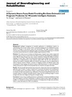
based on the sensor noise and operator scale. Figure 1
depicts the critical value function c
1
(s
1
) for different
noise levels and different Type I error rates. It is easy to
observe that c
1
(·) is a non-negative monotonically
decreasing function of s
1
, which is helpful in detecting
blurred boundaries. Comparing Figure 1a and 1b, we
notice that c
1
(s
1
) is more sensitive to the standard
deviation of sensor noise s
n
than to the Type I error a
I
.
Furthermore, c
1
(s
1
)growsass
n
increases, for eliminat-
ing spurious edges in the presence of highly c orrupted
images. In this article, a thin-plate smoothing spline
model is used to smooth a given image. It is assumed
that the model whose generalized cross-validation scor e
is minimum can pr ovide the variance of the sensor
noise s
n
[58].
For the MRS algorithm, how to sample the scale space
is an open question. In scale space theory and for nat-
ural images, it is known that logarithmic scale is suffi-
cient to represent the scale space completely [13]. For
example, Elder and Zucker [18] used six logarithmic
scales s
1
= {0.5, 1, 2, 4, 8, 16} in their experimen ts.
Table 1 summarises the alternative sampling schemes
for scale space, both the Logarithmic and Limited-Log
methods are logarithmic scales, while the latter has a
shorter coverage. The Linear method samples the scale
uniformly, and the Linear-Log one is a combina tion of
Linear and Logarithmic. In this work, we empirically
found the following linear sampling gives good results:
s
1
= {0.6, 0.9, 1.2, 1.5, , 2.4}. In our implementation, we
select the MRS at each pixel as the smallest scale at
which the gradient estimate exceeds the critical value
function:
ˆσ
1
x, y
=inf
σ
1
:
∇I
x, y, σ
1
≥ c
1
(
σ
1
)
(23)
Strictly speaking, if
∇I
x, y, σ
1
< c
1
(
max
(
σ
1
)
)
,the
pixel usually resides in homogeneous regions and the
MRS can be defined as
ˆσ
1
=max
(
σ
1
)
,while
∇I
x, y, σ
1
> c
1
(
min
(
σ
1
)
)
, the pixel may correspond
(
a
)
(b)
Figure 1 Plots of the critical value function for different parameters settings. (a) The critical value function with respect to different noise
levels (a
I
= 0.05). (b) The critical value function with respect to different Type I error rates (s
n
= 20).
Wang et al. EURASIP Journal on Advances in Signal Processing 2011, 2011:22
/>Page 5 of 19
to edge or detailed feature and the MRS is chosen as
ˆσ
1
= min
(
σ
1
)
.
Finally, w e define the scale-based classifica tion map R
(x, y) as follows:
R
x, y
∈
⎧
⎨
⎩
homogeneous region if ˆσ
1
x, y
≥ σ
smoot
h
edge region if ˆσ
1
x, y
≤ σ
edge
detail reg ion otherwise
(24)
where R(x, y ) denotes the region type of pixel (x, y). It
has to be noted that the proper modulation of the
thresholds s
smooth
and s
edge
is required for a robust
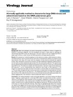
classificat ion map. As an example, the classification map
of the Cameraman image and its noisy version (s
2
=
225) are illustrated in Figures 2b and 2d, respectively. In
the map, black regions are homogeneous, gray regions
represent detail regions, while white regions manifest
Table 1 Alternative sampling of the scale space.
Sample method s
1
Logarithmic {0.5, 1, 2, 4, 8, 16}
Linear {0.5, 1, 1.5, 2, 2.5, 3}
Limited-Log {0.5, 1, 2}
Linear-Log {0.5, 1, 2, 3, 4, 5}
(a) (b)
(
c
)
(
d
)
Figure 2 Local scale- based classification map of the Cameraman image. (a) Original image. (b) Classification map of (a) (s
smooth
=2,s
edge
= 1). (c) Noisy image (s
2
= 225). (d) Classification map of (c) (s
smooth
=2,s
edge
= 1).
Wang et al. EURASIP Journal on Advances in Signal Processing 2011, 2011:22
/>Page 6 of 19
inhomogeneities that indicate most of the important fea-
tures, e.g., the camera and tripod. This example clearly
illustrates that the scale-based classification map readily
indicate locations of highly h omogeneous, detail and
edge regions.
3.2 Scale-based forward-and-backward diffusion
coefficient
As shown in [59,60], if the weight a in (10-11) is con-
stant for all pixels in an image, this diffusion coefficient
(10) is positive for small image gradi ents, while it
becomes negative for large ones, and finally becomes
positive again. Different nonlinear diffusion behaviours
can be obtained by varying the value of a. For example,
when a is large, the backward diffusion force is domi-
nant. The larger a is, the more sharpening occurs. How-
ever, a too large a easily results in oscillations.
Conversely, when a is small, the diffusion process per-
forms image smoothing. Small values of a increase the
noise attenuation a t the price of a possible increase of
detail blur. Thus, the optimal choice depends on the
amount of no ise variance and is typically a trade-off
between smoothing and sharpening. Nevertheless, Gil-
boa et al. [38] propo sed that the same a is used for the
entire image, regardless of local structures of an image,
which leads to over-smoothing in edge or detail regions
and under-smoothing in homogeneous regions. In this
article, we propose the balancing weight a, with differ-
ent values δ
smooth
, δ
edge
and δ
detail
, selectively applied at
each pixel following the value of the local scale-based
classificati on map R(x, y). Indeed, in the edge areas, the
image requires more sharpening to highlight important
features embedded in it, while in the detail regions, the
diffusion process should compromise the effects of
smoothing and sharpening, ensuring that the backward
force can emphasize the fine structures in the image
and the stabilizing forward force is strong enough to
avoid oscillations. Whereas, in homogeneous regions,
the gradient magnitude is very slow after the Gaussian
pre-smoothing is applied to reduce the background
noise. Thus, the approximate i sotropic diffusion is per-
formed to uniformly smooth the gentle and flat areas. In
this way, each pixel is adaptively assigned a d ifferent
parameter by evaluating the local structures. This is
made possible using the MRS-based diffusivity function:
c
∇I
x, y, t
=
1
1+
∇I
x, y, t
/k
f
2
−
α
1+
∇I
x, y, t
/k
b
2
(25)
with
α =
⎧
⎨
⎩
δ
smooth
R
x, y
∈ homogeneous region
s
δ
edge
R
x, y
∈ edge regions
δ
detail
R
x, y
∈ detail regions
(26)
where δ
smooth
, δ
edge
and δ
detail
are the scale-based
weights, selected empirically such that δ
edge
≥ δ
detail
≥
δ
smooth
≥ 0. K
f
and k
b
control the MRS-based diffusiv-
ity function for forward and backward diffusion,
respectively. A s mentioned above, the parameter k
f
has
the same role as the gradient threshold in the P-M dif-
fusion equation. Thus, the mean of local intensity dif-
ferences in homogeneous regions is effective for
controlling the forward diffusion; while k
b
is deter-
mined by the value of the gradient that is emphasized.
Previous works [38,59] demonstrated that k
b
is several
times larger than k
f
, in our case, we empirically defined
the two gradient thresholds in (25) as [k
f
, k
b
] = [1,2]*k.
This strategy is indeed required in cases of natural sig-
nals or images be cause of their nonstationary structure.
Usually, a minimal value of forward diffusion should
be kept, so that large smooth areas do not become
noisy. For the estimation of k, we use the assumption
of i.i.d. noise, indeed, since the noise is assumed to be
randomly distributed in the image space, a practical
way of estimating its variance is to consider homoge-
neous regions where small variations or textures are
mainly due to noise. Thus, k is estimated as the mean
of the local intensity differences on the homogeneity
map, i.e.,
k =
(
x,y
)
∈
h
,
(
i,j
)
∈B
xy
I
i, j
− I
x, y
N
h
(27)
where
h
=
x, y
: ˆσ
1
x, y
≥ σ
smooth
and B
xy
is
the neighbourhood set of pixel (x, y), and N
h
is the total
number of pixels in the homogeneous regions as defined
by the cl assification map R(x, y). When Ω
h
is empty, the
simplest idea might be to setup k as a user defined con-
stant, or using a “ noise estimator": a h istogram of the
absolute values of the gradient throughout the image is
computed, and k is set greater than or equal to e.g. 90%
value of its integral at each iteration.
3.3 Edge orientation driven discretization scheme
(EODDS)
As mentioned in Sect. 3.1, three different regions are
classified before diffusion evolution. However, edge
orientation is not taken c are in the discrete scheme of
P-M anisotropic diffusion. As a result, they are always
considered to be displaced vertically or horizontally [61].
Moreover, one cannot recognize whether a slight inten-
sity variation is mainly due to a slow varying edge or
noise, so it is unreasonable that both situations are trea -
ted in the same way. The anisotropic diffusion discrete
scheme should be modified to take edge orientations
into account i n the detail and edge regions, i.e. filtering
act ion should be rather st rong er on the direct ion paral-
lel to the edge, and weaker on the perpendicular
Wang et al. EURASIP Journal on Advances in Signal Processing 2011, 2011:22
/>Page 7 of 19
direction. Hence, we discretized the original anisotropic
diffusion equation as follows:
I
x, y, t +1
= I
x, y, t
+ λ ·
(
W
V
(
θ
)
·
(
c
N
·∇
N
I + c
S
·∇
S
I
)
+ W
H
(
θ
)
·
(
c
E
·∇
E
I + c
W
·∇
W
I
))
+
λ ·
W
D
1
(
θ
)
·
(
c
NE
·∇
NE
I + c
SW
·∇
SW
I
)
W
D
2
(
θ
)
·
(
c
NW
·∇
NW
I + c
SE
·∇
SE
I
)
(28)
where the mnemonic subscripts N, S, E, W, NE, SW,
NW and SE denote the eight directions North, South,
East, West, North-East, South-West, North-West and
South-East, and the symbol ∇ stands for nearest-neigh-
bour differences. l is the time step for the numerical
scheme; θ istheedgedirectionatpixel(x, y), W
V
(θ),
W
H
(θ),
W
D
1
(
θ
)
and
W
D
2
(
θ
)
are weights for different
edge directions.
For a nonlinear diffusion scheme, stability is an impor-
tant issue that concerns possible unbounded growth or
boundness of the final result of the diffusion scheme.
The essential criterion defining stability is that the
numerical process must restrict the amplification of all
components from the initial conditions. In the following,
we describe how to find the maximum value of l assur-
ing the stability. Assuming N
d
the dimension of the
neighborhood in direction d (in the vertical or horizon-
tal direction for 4-connected neighbourhood, N
d
=1),
the stability condition is given by [30]:
0 ≤ λ ≤
1
D
d=1
2
N
2
d
where D is the dimension of a given image. For our
case (2-D images and 8-connected neighborhood), the
condition becomes:
0 ≤ λ ≤
1
D
d=1
2
N
2
d
=
1
4
d=1
2
N
2
d
=
1
2
1
2
+
2
1
2
+
2
1
2
+
2
1
2
=
1
8
In this article, the step of keypoint orientation in
scale-invariantfeaturetransform(orSIFT)[62]algo-
rithm is used for estimating the edge direction. The
image is subdivided i nto nonoverlapping blocks of the
same size, typically betwee n 8 × 8 and 32 × 32 pixels.
The gradient-based edge orientation histogram is then
calculated in each block. If we let N be the total number
of pixels in the image and n be the total number of bins,
the histogram H
i
meets the following conditions:
N =
n
i
=1
H
i
x, y
(29)
In the histogram, 360 degree is grouped in 36 groups,
each of which is π/18 degree, and we obtain n =36.
Thus, the main orientation in each block is defined as
follows:
θ = ϑ +
π
2
= arctan
index ·
π
18
+
π
2
(30)
and
index = arg max
i
i : H
i
x, y
(
i = 1, 2, 36
)
(31)
where ϑ is the main gradient direction, by calculating
the histogram of the gradient direction for each pixel (x,
y) in the block, and “arctan” is the inverse tangent func-
tion. We assume that if an intensity variation between
two zones is present, the edge has to be located along
the perpendicular direction. The calculation of orienta-
tion histogram can be perfo rmed in real time. Further-
more, the comparison of orientation histograms can be
performed using Euclidian distance that is very fast to
compute for vectors whose dimensions are 36.
Once the estimation of the edge direction has been
performed, the weights W
v
(θ), W
H
(θ),
W
D
1
(
θ
)
and
W
D
2
(
θ
)
have to be defined, in such a way that they
satisfy the following constraint, with the aim of main-
taining the numerical stability of the process:
W
V
(
θ
)
·
(
c
N
+ c
S
)
+ W
H
(
θ
)
·
(
c
E
· +c
W
)
+ W
D
1
(
θ
)
·
(
c
NE
+ c
SW
)
+W
D
2
(
θ
)
·
(
c
NW
+ c
SE
)
≤
1
λ
(32)
In order to illustrate the way the weights are esti-
mated, we divide the x - y plane into five domains as
follows (see Figure 3):
=
⎧
⎪
⎪
⎨
⎪
⎪
⎩
0
0 ≤ θ ≤ π
8or7π
8 ≤ θ ≤ π,
1
π
8 ≤ θ ≤ 3π
8,
2
3π
8 ≤ θ ≤ 5π
8,
3
5π
8 ≤ θ ≤ 7π
8,
(33)
Figure 3 Relating edge direction to direction in an image.
Wang et al. EURASIP Journal on Advances in Signal Processing 2011, 2011:22
/>Page 8 of 19
Taking the constraint (32) and the trigonometric rela-
tion into account, the weights W
v
(θ), W
H
(θ),
W
D
1
(
θ
)
and
W
D
2
(
θ
)
are estimated as:
W
V
(
θ
)
=
⎧
⎨
⎩
0 θ ∈
1
or θ ∈
3
cos
2
θθ∈
0
sin
2
θθ∈
2
(34)
W
H
(
θ
)
=
0 θ ∈
1
or θ ∈
3
1 − W
V
(
θ
)
otherwise
(35)
W
D
1
(
θ
)
=
⎧
⎨
⎩
cos
2
θ − π
4
θ ∈
1
sin
2
θ + π
4
θ ∈
3
0otherwise
(36)
W
D
2
(
θ
)
=
0 θ ∈
0
or θ ∈
2
1 − W
D
1
(
θ
)
otherwise
(37)
For instance, if θ Î Ω
0
, substituting these weights in
the modified anisotropic diffusion Equation 29 leads to
the following:
I
x, y, t +1
= I
x, y, t
+ λ ·
cos
2
θ ·
(
c
N
·∇
N
I + c
S
·∇
S
I
)
+sin
2
θ ·
(
c
E
·∇
E
I + c
W
·∇
W
I
)
(38)
In this case, the edge orientation should approximate
the vertical direction accordi ng to the fact that the edge
direction is always perpendicular to the gradient direc-
tion. During the diffusion process, a relatively large
weight cos
2
θ is assigned in the vertical direction to guar-
antee that t he diffusion should mainly occur in the
direction parallel to the edge, while a relatively small
weight sin
2
θ is assigned in the horizontal direction to
ultimately avoid diffusion across the edge.
3.4 SFABD algorithm
The algorithm for the proposed SFABD scheme is sum-
marised in Algorithm 1.
4. Experiments
Chen [63] classified the existing performance evaluation
methods into three categories; i.e. subjective, objective
and application-based methodologies. By the s ubjective
methodology, a noisy image and its enhance d images
are illustrated. Thus, the evaluation on the performance
of an algorithm is dependent on human ’ s c ommon
sense gained from very much sophisticated visual per-
ception experience. By the objective methodology, an
evaluation is performed by comparing the enhanced
image and its original uncorrupted version to see how
much noise has been removed from a noisy image. By
the application-based methodology, images in a certain
application field are used for test and the enhancing
results are assessed by a specialist who has expertise in
the field or a comparison with an anticipated result set
up prior to the test.
To assess the proposed approach, we follow the
above-described methodology and demonstrate the
effectiveness of SFABD in enhancing fine edge struc-
tures, i.e. we applied it to a variety of blurred and noisy
images by comparing its results to five counterparts,
namely, the Catte’s anisotropic diffusion (CAD) [19], the
robust anisotropic diffusion (RAD) [29], the Monteil’ s
anisotropic diffusion (MAD) [33], the Weickert’saniso-
tropic diffusion (WAD) [54], and the edge-enhancing
diffusion (EED) [30]. The gradient threshold k should be
chosen according to the noise level and the edge
strength. In our experiments, we set k in different diffu-
sion algorithms by referring t o the original papers. The
ultimate goal of image enhancement is to facilitate the
subsequent processing for early vision. To demonstrate
the usefulness of our algorithm in an early vision task,
we apply our algorithm for performing edge-enhancing
filtering on medical images, for an application-based
evaluation.
In order to objectively evaluate the performance of
the different diffusion algorithms, we adopt two
noise-reduction measures: peak signal-to-noise ratio
(PSNR) and the universal image quality index (UIQI).
The measure of PSNR has been widely used in evalu-
ating performance of a smoothing algorithm in the
objective methodology. For a given noisy image I, I(i,
j, T) denotes the intensity of pixel (x, y) Î I at itera-
tion T while an anisotropic diffusion algorithm is
applied to the noisy image. G(i, j) is its uncorrupted
ground-truth. As a result, the PSNR is defined as fol-
lows:
PSNR = 10 ·log
10
⎛
⎜
⎜
⎝
i,j
MAX
2
I
i,j
G
i, j
− I
i, j, T
2
⎞
⎟
⎟
⎠
dB
(39)
Here, MAX
I
is the maximum gray value of the image.
When the pixels are represented using 8 bits per sam-
ple, MAX
I
= 225. Typical values for the PSNR in lossy
image and video compression are between 30 and 50
dB, where higher is better. Acceptable values for wire-
less transmissi on quality loss are considered to be about
20 to 25 dB [64,65]. Recently, the UIQI has been used
to better evaluate image quality due to its strong ability
in measuring structural distortion occurred during the
image degradation processes [66]:
Q =
1
M
j
M
=
1
Q
j
(40)
Wang et al. EURASIP Journal on Advances in Signal Processing 2011, 2011:22
/>Page 9 of 19
where M is the t otal step number and Q
j
denotes the
local quality index com puted within a sliding window.
In this article, a sliding window of size 8 × 8 is applied
to estimate an entire image. The dynamic range of Q is
[-1,1], the value 1 is on ly achieved if the compared
images are identical and the value of -1 means lowest
quality of the distorted image.
4.1 General images
The performance of the proposed algorithm is evaluated
using four standard images of size 512 × 512 and 256
gray-scale values. The image of Peppers is employed as
an example of piecewise-constant image. The Lena and
Cameraman images are two examples with both textures
and smooth regions. The Boat image is an example with
different edge features. For performance evaluation, the
images have been corrupted with additive Gaussian
whitenoisewithdifferentnoiselevels.ThePSNRand
UIQI values of the four noisy images with respect to dif-
ferent noise variance are listed in Table 2. The Lena and
Boat images and their noisy versions with noise variance
225 are displayed in Figures 4 and 5 , respectively. For
clarity, only selected regions of the images are displayed.
Figures 6 and 7 depict the restored images using the
six algorithms, for visual quality assessment. The
results yielded by CAD and WAD schemes are
depicted in Figures 6a, b and 7a, b, respectively. Both
methods can well clean noise but blur the details of
the restored results, such as t he hat, its decoration and
the hair in the image of Lena (see Figure 4a)), and the
ground texture at the end o f the Boat image of (see
Figure 5a). This conforms our analysis that using the
gradient, as only local discontinuity measure, would
yield difficulties in distinguishing betw een edge details
and noise and detecting fine structure. For RAD, a lot
of noise still survives in the restored images. The
restored results indicate that this method is very sensi-
tive to noise. In Figures 6d and 7d, very large oscilla-
tions of gradient introduced by noise canno t be fully
attenuated by MAD. The two resultant images present
insufficient diffusion for restoration, in which the
homogeneous background, such as Lena’ s face and
bare shoulder (see Figure 4a) and the sky in the Boat
image (see Figure 5a), cannot be completely eliminated
because the diffusion process is terminated in early
iterations. A better edge-preserving filtering is yielded
by the EED process and the corresponding results are
shown in Figures 6e and 7e, respectively. Finally, the
images produced by the proposed SFABD scheme are
represented in Figures 6f and 7f, respectively. The
Table 2 PSNR (In dB) and UIQI of the noisy testing images of Peppers, Lena, Cameraman and Boat with respect to
different noise variances
Image Noise variance (s
2
)
100 225 400 625 900
PSNR UIQI PSNR UIQI PSNR UIQI PSNR UIQI PSNR UIQI
Peppers 28.16 0.5411 24.71 0.4087 22.22 0.3232 20.31 0.2646 18.82 0.2237
Lena 28.14 0.5024 24.60 0.3891 22.15 0.3137 20.22 0.2617 18.70 0.2221
Cameraman 28.27 0.3806 24.86 0.3066 22.45 0.2585 20.56 0.2227 19.03 0.1945
Boat 28.13 0.6322 24.63 0.5031 22.17 0.4132 20.27 0.3467 18.73 0.2960
(
a
)
(
b
)
Figure 4 Lena image. (a) Original image. (b) Noisy image with a
noise variance of 225.
(
a
)
(
b
)
Figure 5 Boat image. (a) Original image. (b) Noisy image with a
noise variance of 225.
Wang et al. EURASIP Journal on Advances in Signal Processing 2011, 2011:22
/>Page 10 of 19
(a)
(b) (c)
(
d
)
(
e
)
(
f
)
Figure 6 Enhanced Lena image. (a) CAD . (b) WAD. (c) RAD. (d) MAD (g =0.1).(e) EED. (f) SFABD (s =0.1,s
smooth
=2,s
edge
=1,δ
smooth
=
0.3, δ
edge
= 0.6, δ
edge
= 0.9) (10 iterations).
(a) (b) (c)
(
d
)
(
e
)
(
f
)
Figure 7 Enhanced Boat image. (a) CAD. (b) WAD. (c) RAD. (d) MAD (g =0.1).(e) EED. (f) SFABD (s =0.1,s
smooth
=2,s
edge
=1,δ
smooth
=
0.3, δ
detail
= 0.6, δ
edge
= 0.9) (10 iterations).
Wang et al. EURASIP Journal on Advances in Signal Processing 2011, 2011:22
/>Page 11 of 19
noise is removed and this is d ue to the forward diffu-
sion.Meanwhile,edgefeatures, including most of the
fine details, are sharply reproduced. By comparing the
resultant images of SFABD with the other five classical
algorithms, we can notice that the SFABD algorithm
achieves better visual qua lity. The reason for this is
twofold: First, the multiscale discontinuity measure of
the MRS-based diffusivity function is more effective
than the gradient in detecting edge features and fine
structure under a noisy environment, which is helpful
for correctly classifying regions and estimating the gra-
dient thresholds. Second, the proposed diffusion
method incorporates both of the two discontinuity
measures in the FAB diffusion coefficient by adopting
a scale-based weight for balancing the forward diffu-
sion and backward one. This strategy c an ensure the
elegant property of effectively smoothing noise while
simultaneously sharpening edges and fine details of a
noisy image. Table 3 lists the PSNR and UIQI values
that are reported by the different algorithms, applied
on the test images with different noise levels. For clar-
ify, a noise variance of 400 is used for comparison.
The experimental results demonstrate that the SFABD
scheme can efficiently improve the PSNR value by
around 8.6 dB better than the other algorithms. Addi-
tionally, the proposed diffusion scheme can produce an
image with around 22% less structural distortion
according to the UIQI values, which is the best among
Table 3 PSNR of the six diffusion algorithms for the noisy testing images of Peppers, Lena, Cameraman and Boat with
respect to different noise variances
Scheme Image Noise variance (s
2
)
100 225 400 625 900
PSNR UIQI PSNR UIQI PSNR UIQI PSNR UIQI PSNR UIQI
CAD Peppers 32.93 0.5917 31.90 0.5681 30.81 0.5367 29.81 0.5040 28.93 0.4737
Lena 33.48 0.6518 31.16 0.6118 31.08 0.5733 30.06 0.5339 29.12 0.4961
Cameraman 34.55 0.5819 32.89 0.5138 31.43 0.4588 30.06 0.4156 28.81 0.3806
Boat 30.87 0.6252 30.03 0.6048 29.18 0.5816 28.31 0.5507 27.55 0.5252
WAD Peppers 32.57 0.5771 31.60 0.5553 30.61 0.5287 29.67 0.5001 28.87 0.4719
Lena 32.98 0.6345 31.84 0.6036 30.80 0.5667 29.87 0.5309 29.00 0.4959
Cameraman 33.96 0.5619 32.51 0.4984 31.13 0.4487 29.84 0.4072 28.67 0.3722
Boat 30.55 0.6022 29.73 0.5814 28.88 0.5579 28.09 0.5318 25.37 0.5078
RAD Peppers 31.44 0.6165 28.27 0.4995 25.82 0.4118 23.95 0.3496 22.50 0.3042
Lena 31.91 0.6174 28.36 0.4931 25.88 0.4095 23.98 0.3525 22.46 0.3085
Cameraman 32.60 0.4944 28.81 0.3868 26.21 0.3278 24.23 0.2854 22.61 0.2538
Boat 31.46 0.7036 28.33 0.6037 25.87 0.5164 23.98 0.4460 22.42 0.3927
MAD Peppers 32.66 0.6025 30.84 0.5538 28.97 0.4930 27.28 0.4373 25.95 0.3919
Lena 33.32 0.6583 31.19 0.5886 29.19 0.5137 27.54 0.4552 26.09 0.4046
Cameraman 34.15 0.5809 31.63 0.4773 29.24 0.3990 27.33 0.3453 25.77 0.3071
Boat 31.25 0.6475 29.74 0.6103 28.14 0.5599 26.63 0.5050 25.34 0.4578
EED Peppers 33.04 0.6130 31.62 0.5754 30.15 0.5274 28.88 0.4832 27.76 0.4447
Lena 33.85 0.6702 32.11 0.6128 30.60 0.5608 29.23 0.5104 28.01 0.4656
Cameraman 34.77 0.5952 32.72 0.5088 30.87 0.4508 29.28 0.4045 27.90 0.3690
Boat 31.28 0.6655 30.26 0.6348 29.14 0.6018 28.08 0.5613 27.07 0.5282
SFABD
(without EODDS)
Peppers 32.94 0.5977 31.82 0.5662 30.80 0.5366 29.90 0.5071 28.99 0.4743
Lena 33.76 0.6612 32.13 0.6135 30.95 0.5725 30.01 0.5338 29.24 0.5032
Cameraman 35.06 0.5947 33.01 0.5159 31.41 0.4572 30.17 0.4205 29.05 0.3858
Boat 31.44 0.6496 29.92 0.6043 28.79 0.5681 27.93 0.5363 27.20 0.5093
SFABD
(with EODDS)
Peppers 33.33 0.6210 32.03 0.5801 30.90 0.5407 30.08 0.5109 29.35 0.4789
Lena 34.24 0.6763 32.51 0.6195 31.21 0.5737 30.28 0.5378 29.67 0.4957
Cameraman 35.64 0.6006 33.58 0.5222 31.73 0.4654 30.53 0.4250 29.46 0.3929
Boat 31.87 0.6805 30.69 0.6363 29.49 0.6090 28.55 0.5684 27.59 0.5330
For the SFABD, the parameters settings are: s
smooth
=2,s
edge
=1,δ
smooth
= 0.3, δ
detail
= 0.6, δ
edge
= 0.9
Wang et al. EURASIP Journal on Advances in Signal Processing 2011, 2011:22
/>Page 12 of 19
the six algorithms. Thus, we can say that the SFABD
scheme outperforms the state-of-the-art diffusion
methods. In addition, the performance of the EODDS
has also been revealed in Table 4. It is evident that our
algorithm using EODDS has achieved better statistical
results than that of our algorithm without it, which
confirms the valid ity of the EODDS.
Second, the proposed SFABD algorithm has been also
compared to three existing FAB diffusion schemes,
name ly the GSZFABD [38], LVCFA BD [44] and tunable
FAB diffusion (TFABD) [47], using visual quality and
the PSNR and UIQI values. Figure 8 depicts the
obtained results of the consi dered FAB diffusion
schemes. One can notice that all the four FAB processes
Table 4 PSNR of the four FAB diffusion schemes for the noisy testing images of Peppers, Lena, Cameraman and Boat
with respect to different noise variances
Scheme Image Noise variance (s
2
)
100 225 400 625 900
PSNR UIQI PSNR UIQI PSNR UIQI PSNR UIQI PSNR UIQI
FABD Peppers 32.47 0.5922 31.73 0.5677 30.90 0.5373 29.98 0.5068 29.16 0.4831
Lena 32.58 0.6488 31.94 0.6098 30.70 0.5543 30.25 0.5374 29.35 0.4940
Cameraman 33.55 0.5754 32.74 0.5127 31.60 0.4559 30.39 0.4227 29.21 0.3928
Boat 29.38 0.6137 29.07 0.5991 28.59 0.5783 27.81 0.5426 27.29 0.5163
LVCFABD Peppers 32.35 0.6207 31.74 0.5732 30.30 0.5249 29.54 0.4914 28.24 0.4468
Lena 33.27 0.6769 32.37 0.6138 31.05 0.5699 29.91 0.5201 28.40 0.4635
Cameraman 34.34 0.5905 33.48 0.5155 31.68 0.4606 30.22 0.4169 28.61 0.3785
Boat 31.42 0.6994 30.49 0.6352 29.28 0.6087 28.39 0.5668 27.30 0.5293
TFABD Peppers 32.85 0.6044 31.98 0.5703 30.67 0.5336 30.01 0.5054 29.24 0.4763
Lena 33.72 0.6711 32.50 0.6181 31.09 0.5702 30.27 0.5372 29.42 0.5052
Cameraman 35.31 0.5980 33.41 0.5197 31.69 0.4648 30.42 0.4235 29.39 0.3937
Boat 31.72 0.6689 30.56 0.6487 29.34 0.6019 28.40 0.5719 27.58 0.5212
SFABD
(with EODDS)
Peppers 33.33 0.6210 32.01 0.5801 30.90 0.5407 30.08 0.5109 29.35 0.4789
Lena 34.24 0.6763 32.51 0.6195 31.21 0.5737 30.28 0.5378 29.67 0.4957
Cameraman 35.64 0.6006 33.58 0.5222 31.73 0.4654 30.53 0.4250 29.46 0.3929
Boat 31.87 0.6805 30.69 0.6363 29.49 0.6090 28.55 0.5684 27.59 0.5330
For the SFABD, the parameters settings: s
smooth
=2,s
edge
=1,δ
smooth
= 0.3, δ
detail
= 0.6, δ
edge
= 0.9
(a) (b) (c)
(
d
)
(
e
)
(
f
)
Figure 8 Peppers image. (a) Original image. (b) Noisy image with a noise variance of 225. (c) Enhanced with GSZFABD. (d) LVCFABD. (e)
TFABD. (f) SFABD. (s = 0.1, s
smooth
=2,s
edge
=1,δ
smooth
= 0.3, δ
detail
= 0.6, δ
edge
= 0.9) (10 iterations).
Wang et al. EURASIP Journal on Advances in Signal Processing 2011, 2011:22
/>Page 13 of 19
can achieve a good compromise between sharpening
and denoising. However, as illustrated in F igure 8a, the
GSZFABD process blurs edges and de tail features. From
Figures 8b, c, it can be seen that the LVCFABD and
TFABD schemes are sensitive to noise: the LVCFABD
results in developing singularities in homogeneous
regions, such as the inner parts of peppers, while the
TFABD causes oscillations in the vicinity of edges, e.g.
the outer contour of peppers. However, the proposed
SFABD scheme exhibits the best edge-enhancing diffu-
sion behaviour. The quantitative results of the four
schemes are given in Table 4. It is evident from Table 4
that the SFABD scheme is much more efficient than the
other three schemes for the four images. Hence, we can
say that SFABD outperforms the existing FAB enha nce-
ment techniques.
In order to appraise the effect iveness of the adaptive
gradient threshold, the gradient threshold k
f
curves for
four noisy images (s
2
= 400) are depicted in Figure 9. It
can be seen that all the curves, representing the evolution
of this parameter, share the same decreasing behaviour as
already demonstrated in other works, allowing lesser and
lesser gradients to take part in the diffusing process.
Moreover, after 20 iterations, k
f
decreases slower and
slower and the scheme converges to a steady state where
for t ® ∞,wegetc(|∇I|) ® 0, whi ch means that almost
no diffusion is performing. Note that, the estimation of
an optimum threshold value k has been addressed by sev-
eral authors [29,50,67,68]. However, to our knowledge,
these authors do not explain how to determine the
homogenous regions during the process. In this work, an
appropriate solution for automatically adapting the gradi-
ent threshold at each iteration has been proposed.
4.2 Medical images
In medical images, low SNR and CNR often degrade the
information and affect several i mage processing tasks,
such as segmentation, classification and registration.
Therefore, it is of considerable interest to improve SNR
and CNR to reduce the deterioration of image informa-
tion. In this section, we report the results of the proposed
SFABD scheme on two three-dimensional MR images
[69,70], both of which have been simulated using two
sequences (T1- and T2-weighted) with 1 mm of slice
thickness, 9% noise level and 20% of intensity non-unifor-
mity downloaded from Brainweb [71] using default acqui-
sition parameters for each modality. These simulations are
based on an anatomical model of normal brain, which can
serve as ground truth for any analysis procedure.
Figures10and11showtwoexamplesofenhanced
MR image using different diffusion schemes. The origi-
nal noise-free images and their corrupt ed versions are
illustrated in Figures 10a, b and 11a, b, respectively. As
expected, the six algorithms remove noise and simulta-
neously smooth the homogeneous regions, such as
white matter. Howeve r, for RAD, noise is still remain-
ing in the resulting images. Some structure details are
not visible in the images restored by the CAD, WAD
and MAD algorithms, though they can greatly attenu-
ate the eff ect of noise. According to the visual analyses
of the image quality, the results given by the EED dif-
fusion and the proposed SFABD are comparable,
because the two processes p erform edge-enhancing dif-
fusion. Nevertheless, the SFABD scheme achieves bet-
ter contrast and produces more reliable edges, which is
especially useful for segmentation a nd classification
purposes necessary in medical image applications.
In order to objectively evaluate the performances of the
different diffusion al gorithms on medical images, we
adopt the PSNR and the Structural Similarity (SSIM)
measure [72]. SSIM is a quality metric that measures the
presence of the image structure details in the restored
images and the value one is only achieved if the com-
pared images are identical. The lowest value is zero if the
images show no similarity at all. Since both the consid-
ered MR simulated images are three-dimensional data
volume, we compare the PSNR and SSIM values at each
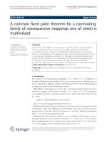
slice for objective evaluation. As shown in Figure 12, the
PSNR values of the restored images achieved by the pro-
posed SFABD scheme are comparable or higher than the
other diffusion algorithms, and the SSIM values o f
SFABD are significantly higher. Finally, the proposed
scheme enhances boundary sharpness and fine structures
better than other considered diffusion methods.
5. Conclusion
We have presen ted a novel SFABD scheme for image
restoration and enhancement. In the proposed scheme,
Figure 9 Gradient threshold evolution curves for the noisy test
images Peppers, Lena, Cameraman and Boat (noise variance
400).
Wang et al. EURASIP Journal on Advances in Signal Processing 2011, 2011:22
/>Page 14 of 19
the magnitude of the diffusion coefficients at each pixel is
determined by taking into account the property of the
image through scale-space, using a classification map
obt ained via the MRS. According to the type of the con-
sidered pixel (belonging to a homogenous, detail or edge
region), a variable weight is incorporated into the anisotro-
pic diffusion PDE to adaptively encourage strong smooth-
ing in homogeneous regions and suitable sharpening in
detail and edge regions. Moreover, we propose a method
to estimate the parameter k of MRS-based diffusivity
function, as the mean of the local intensity differences on
homogeneous regions as determined by the MRS-based
classification map. Finally, a numerical scheme, taking into
account the edge orientation has been proposed. Further-
more, ext ensive qualitati ve and quantitative comparisons
with a variety of existing diffusion schemes demonstrate
the effectiveness of the proposed scheme, along with its
potential use for medical image applications. Future work
will involve two main aspect of the proposed approach,
namely an adaptive approach for the estimation of the
(a) (b)
(c) (d) (e)
(
f
)
(g)
(
h
)
Figure 10 Enhanced images for the 3-dimensional data volume of a T1-weighted MR simulated image. (a) Original MR image (slice 80).
(b) Corrupted MR image. (c) Enhanced MR image with CAD. (d) WAD. (e) RAD. (f) MAD (g = 0.1). (g) EED. (h) SFABD (s = 0.1, s
smooth
=2,s
edge
=1,δ
smooth
= 0.2, δ
detail
= 0.4, δ
edge
= 0.6) (10 iterations).
Wang et al. EURASIP Journal on Advances in Signal Processing 2011, 2011:22
/>Page 15 of 19
parameters, as well as establishing an automatic stopping
criterion to replace the pref ixed numbers of iterati on for
anisotropic diffusion.
Algorithm 1. Scale-based forward-and-backward
diffusion
1. Initialize the image data I. I (x, y, 0) denotes the origi-
nal intensity of pixel (x, y).
2. Initialize the diffusion parameters. Set the values of
theofthenoisescales, the maximum number of
iterations T, the classification map thresholds s
smooth
and
s
edge
, and the scale-based weights δ
smooth
, δ
edge
and δ
detail
.
3. Calculate the critical value for each pixel and deter-
mine its region type.
a. Obtain the regularized image I
s
.
b. Compute the gradient of the smoothed image, ∇I
s
=(d
x
,d
y
)
T
.
c. Calculate the critical value for each pixel.
(a) (b)
(c) (d) (e)
(
f
)
(g)
(
h
)
Figure 11 Enhanced images for the 3-dimensional data volume of a T2-weighted MR simulated image. (a) Original MR image (slice 80).
(b) Corrupted MR image. (c) Enhanced MR image with CAD. (d) WAD. (e) RAD. (f) MAD (g = 0.1). (g) EED. (h) SFABD (s = 0.1, s
smooth
=2,s
edge
=1,δ
smooth
= 0.2, δ
detail
= 0.4, δ
edge
= 0.6) (10 iterations).
Wang et al. EURASIP Journal on Advances in Signal Processing 2011, 2011:22
/>Page 16 of 19
d. Determine the minimum reliable scale of each
pixel by using the relationship between the spatial
gradient and the critical value (23).
e. Estimate the classification map R(x, y) in (24)
4. Iterate the diffusion filtering until t = T.
a. The gradient thresholds k
f
and k
b
are estimated as
discussed in Section 3.2.
b. Fo r each pixel (x, y), the diffusion coefficient c(∇)
is computed using Eq. (25). In homogeneous and
detail regions, the traditional 4-connected neigh-
bourhood diffusion discretization equation is per-
formed to update I(x, y, t); while in edge regions, the
8-connected neighbourhood diffusion discr etization
equation (28) is performed to update I(x, y, t).
Abbreviations
CAD: Catte’s anisotropic diffusion; CNR: contrast-to-noise ratio; EED: edge-
enhancing diffusion; EODDS: edge orientation driven discr etization scheme;
FAB: forward-and-backward; LVCFABD: local variance controlled forward-and-
backward diffusion; MAD: Monteil’s anisotropic diffusion; MRS: Minimum
Reliable Scale; PDE: partial differential equation; pdf: probability distribution
function; P-M: Perona-Malik; PSNR: peak signal-to-noi se ratio; RAD: robust
anisotropic diffusion; SIFT: scale-invariant feature transform; SFABD: scale-
based forward-and-backward diffusion; SNR: signal-to-noise ratio; SSIM:
Structural Similarity; TFABD: tunable FAB diffusion; UIQI: universal image
quality index; WAD: Weickert’s anisotropic diffusion.
Acknowledgements
This work was supported in part by the National Natural Science Foundation
of China under Grant 40901205, in part by the National Basic Research
Program of China (973) under Grant 2009CB723905, in part by the Special
Fund for Basic Scientific Research of Central Colleges, China University of
Geosciences, Wuhan, under Grant CUGL090210, in part by the Foundation of
Key Laboratory of Geo-informatics of State Bureau of Surveying and
Mapping under Grant 201022, in part by the Foundation of Key Laboratory
of Resources Remote Sensing & Digital Agriculture, Ministry of Agriculture
under Grant RDA1005, in part by the Foundation of Key Laboratory of
Education Ministry for Image Processing and Intelligent Control under Grant
(a) PSNR vs. Slice number diagram (T1- weighted) (b) SSIM vs. Slice number diagram (T1- weighted)
(c) PSNR vs. Slice number diagram (T2- weighted) (d) SSIM vs. Slice number diagram (T2- weighted
)
Figure 12 The PSNR and SSIM measures for the different diffusion algorithms at each slice of the T1- and T2-weighted MR images.
Wang et al. EURASIP Journal on Advances in Signal Processing 2011, 2011:22
/>Page 17 of 19
200908, in part by the Foundation of Digital Land Key Laboratory of Jiangxi
Province under Grant DLLJ201004. The authors would also like to thank the
anonymous reviewers for their valuable comments and suggestions which
significantly improved the quality of this article.
Author details
1
Institute of Geophysics and Geomatics, China University of Geosciences,
People’s Republic of China
2
State Key Laboratory of Information Engineering
in Surveying, Mapping, and Remote Sensing, Wuhan University, People’s
Republic of China
3
Department of Electronics & Informatics (ETRO), Vrije
Universiteit Brussel (VUB), Belgium
Competing interests
The authors declare that they have no competing interests.
Received: 30 November 2010 Accepted: 16 July 2011
Published: 16 July 2011
References
1. N Damera-Venkata, TD Kite, WS Geisler, BL Evans, AC Bovik, Image quality
assessment based on a degradation model. IEEE Trans Image Process. 9(4),
636–650 (2000). doi:10.1109/83.841940
2. F Russo, An image enhancement technique combining sharpening and
noise reduction. IEEE Trans Instrum Meas. 51(4), 824–828 (2002).
doi:10.1109/TIM.2002.803394
3. JS Lee, Digital image enhancement and noise filtering by use of local
statistics. IEEE Trans Pattern Anal Machine Intell. PAMI-2, 165–168 (1980)
4. P Chan, J Lim, One-dimensional processing for adaptive image restoration.
IEEE Trans Acoust Speech Signal Process. 33(1), 117–126 (1985). doi:10.1109/
TASSP.1985.1164534
5. DCC Wang, AH Vagnucci, CC Li, Gradient inverse weighted smoothing
scheme and the evaluation of its performance. Comput Graphics Image
Process. 15(2), 167–181 (1981). doi:10.1016/0146-664X(81)90077-0
6. K Rank, R Unbehauen, An adaptive recursive 2-D filter for removal of
Gaussian noise in images. IEEE Trans Image Process. 1(3), 431–436 (1992).
doi:10.1109/83.148617
7. CB Ahn, YC Song, DJ Park, Adaptive template filtering for signal-to-noise
ratio enhancement in magnetic resonance imaging. IEEE Trans Med
Imaging. 18(6), 549–556 (1999). doi:10.1109/42.781019
8. SM Smith, JM Brady, SUSAN-A New Approach to Low Level Image
Processing. Int J Comput Vision. 23(1), 45–78 (1997). doi:10.1023/
A:1007963824710
9. T Iijima, Basic theory of pattern observation. Papers of Technical Group on
Automata and Automatic Control (1959)
10. T Iijima, Basic theory on normalization of a pattern (in case of typical one-
dimensional pattern). Bull Electr Lab. 26, 368–388 (1962)
11. J Weickert, S Ishikawa, A Imiya, Linear Scale-Space has First been Proposed
in Japan. J Math Imaging Vision. 10(3), 237–252 (1999). doi:10.1023/
A:1008344623873
12. AP Witkin, Scale-space filtering, in Proceedings of International Joint
Conference on Artificial Intelligence, New York, pp. 1019–1021 (1983)
13. JJ Koenderink, The structure of images. Biol Cybern. 50, 363–370 (1984).
doi:10.1007/BF00336961
14. JJ Koenderink, AJV Doorn, Generic neighborhood operators. IEEE Trans
Pattern Anal Machine Intell. 14(6), 597–605 (1992). doi:10.1109/34.141551
15. T Lindeberg, Feature detection with automatic scale selection. Int J Comput
Vision. 30(2), 77–116 (1998)
16. AL Yuille, T Poggio, Scaling theorems for zero-crossings. IEEE Trans Pattern
Anal Machine Intell. 8(1), 15–25 (1986)
17. J Babaud, AP Witkin, M Baudin, RO Duda, Uniqueness of the Gaussian
kernel for scale-space filtering. IEEE Trans Pattern Anal Machine Intell. 8(1),
26–33 (1986)
18. JH Elder, SW Zucker, Local scale control for edge detection and blur
estimation. IEEE Trans Pattern Anal Machine Intell. 20(7), 699–716 (1998).
doi:10.1109/34.689301
19. F Catte, PL Lions, JM Morel, T Coll, Image selective smoothing and edge
detection by nonlinear diffusion. SIAM-JNA. 29(1), 182–193 (1992)
20. L Alvarez, PL Lions, JM Morel, Image selective smoothing and edge
detection by nonlinear diffusion. SIAM-JNA. 29(3), 845–866 (1992)
21. G Gerig, O Kubler, R Kikinis, FA Jolesz, Nonlinear anisotropic filtering of MRI
data. IEEE Trans Med Imaging. 11(2), 221–232 (1992). doi:10.1109/42.141646
22. M Nitzberg, T Shiota, Nonlinear image filtering with edge and corner
enhancement. IEEE Trans Pattern Anal Machine Intell. 14(8), 826–833 (1992).
doi:10.1109/34.149593
23. RT Whitaker, SM Pizer, A multi-scale approach to nonuniform diffusion.
Comput Vision Graphics Image Process Image Underst. 57,99–110 (1993).
doi:10.1006/cviu.1993.1006
24. L Alvarez, L Mazorra, Signal and Image Restoration Using Shock Filters and
Anisotropic Diffusion. SIAM J Numer Anal. 31(2), 590–605 (1994).
doi:10.1137/0731032
25. X Li, T Chen, Nonlinear diffusion with multiple edginess thresholds. Pattern
Recognit. 27(8), 1029–1037 (1994). doi:10.1016/0031-3203(94)90142-2
26. J Weickert, Theoretical foundations of anisotropic diffusion in image
processing. Computing. 11, 221–236 (1996)
27. B Fischl, EL Schwartz, Learning an Integral Equation Approximation to
Nonlinear Anisotropic Diffusion in Image Processing. IEEE Trans Pattern Anal
Machine Intell. 19(4), 342–352 (1997). doi:10.1109/34.588012
28. ST Acton, Multigrid anisotropic diffusion. IEEE Trans Image Process. 7(3),
280–291 (1998). doi:10.1109/83.661178
29. MJ Black, G Sapiro, DH Marimont, D Heeger, Robust anisotropic diffusion.
IEEE Trans Image Process. 7(3), 421–432 (1998). doi:10.1109/83.661192
30. J Weickert, Anisotropic Diffusion in Image Processing (BG Teubner, Stuttgart,
1998)
31. J Weickert, BMTH Romeny, MA Viergever, Efficient and reliable schemes for
nonlinear diffusion filtering. IEEE Trans Image Process. 7(3), 398–410 (1998).
doi:10.1109/83.661190
32. B Fischl, EL Schwartz, Adaptive nonlocal filtering: a fast alternative to
anisotropic diffusion for image enhancement. IEEE Trans Pattern Anal
Machine Intell. 21(1), 42–48 (1999). doi:10.1109/34.745732
33. J Monteil, A Beghdadi, A new interpretation of the nonlinear anisotropic
diffusion for image enhancement. IEEE Trans Pattern Anal Machine Intell.
21(9), 940–946 (1999). doi:10.1109/34.790435
34. ST Acton, Locally monotonic diffusion. IEEE Trans Signal Process. 48(5),
1379–1389 (2000). doi:10.1109/78.839984
35. I Pollak, AS Wilsky, H Krim, Image segmentation and edge enhancement
with stabilized inverse diffusion equations. IEEE Trans Image Process. 9(2),
256–266 (2000). doi:10.1109/83.821738
36. G Sapiro, Geometric Partial Differential Equations and Image Analysis
(Cambridge University Press, Cambridge, 2001)
37. G Aubert, P Kornprobst, Mathematical Problems in Image Processing: Partial
Differential Equations and the Calculus of Variations (Springer Verlag, New
York, 2002)
38. G Gilboa, N Sochen, YY Zeevi, Forward-and-backward diffusion processes
for adaptive image enhancement and denoising. IEEE Trans Image Process.
11(7), 689–703 (2002). doi:10.1109/TIP.2002.800883
39. P Mrázek, M Navara, Selection of Optimal Stopping Time for Nonlinear
Diffusion Filtering. Int J Comput Vision. 52(2/3), 189–203 (2003). doi:10.1023/
A:1022908225256
40. G Gilboa, NSYY Zeevi, Image Enhancement and Denoising by Complex
Diffusion Processes. IEEE Trans Pattern Anal Machine Intell. 25(8), 1020–1036
(2004)
41. S Young-Chul, C Doo-Hyun, Scale-based image enhancement using
modified anisotropic diffusion filter. Opt Eng. 43(9), 2094–2099 (2004).
doi:10.1117/1.1778730
42. D Tschumperle, R Deriche, Vector-valued Image Regularization with PDEs: A
Common Framework for Different Applications. IEEE Trans Pattern Anal
Machine Intell. 27(4), 1–12 (2005)
43. JM Duarte-Carvajalino, PE Castillo, M Velez-Reyes, Comparative Study of
Semi-Implicit Schemes for Nonlinear Diffusion in Hyperspectral Imagery.
IEEE Trans Image Process. 16(5), 1303–1314 (2007)
44. Y Wang, L Zhang, P Li, Local Varianced-Controlled Forward-and-Backward
Diffusion for Image Enhancement and Noise Reduction. IEEE Trans Image
Process. 16(7), 1854–1864 (2007)
45. J Zhong, H Sun, Wavelet-Based Multiscale Anisotropic Diffusion With
Adaptive Statistical Analysis for Image Restoration. IEEE Trans Circuits Syst.
55(9), 2716–2725 (2008)
46. Y Wang, R Niu, X Yu, Anisotropic Diffusion for Hyperspectral Imagery
Enhancement. IEEE Sensors J. 10(3), 469–477 (2010)
47. Y Wang, R Niu, X Yu, L Zhang, H Shen, Image restoration and enhancement
based on tunable forward-and-backward diffusion. Opt Eng. 49(5), 057004.
(1-20) (2010)
Wang et al. EURASIP Journal on Advances in Signal Processing 2011, 2011:22
/>Page 18 of 19
48. A Pizurica, I Vanhamel, H Sahli, W Philips, A Katartzis, Bayesian formulation
of edge-stopping functions in nonlinear diffusion. IEEE Signal Process Lett.
13(8), 501–504 (2006)
49. M Alrefaya, H Sahli, I Vanhamel, HD Nho, A Nonlinear Probabilistic
Curvature Motion Filter for Positron Emission Tomography Images, in
Lecture Notes in Computer Science. 5567, 212–223 (2009). doi:10.1007/978-3-
642-02256-2_18
50. P Perona, J Malik, Scale-space and edge detection using anisotropic
diffusion. IEEE Trans Pattern Anal Machine Intell. 12(7), 629–639 (1990).
doi:10.1109/34.56205
51. C Wyatt, E Bayram, Y Ge, Minimum Reliable Scale Selection in 3D. IEEE
Trans Pattern Anal Machine Intell. 28(3), 481–487 (2006)
52. F Torkamani-Azar, KE Tait, Image recovery using the anisotropic diffusion
equation. IEEE Trans Image Process. 5(11), 1573–1578 (1996). doi:10.1109/
83.541427
53. R Whitaker, G Gerig, Geometrically-Driven Diffusion in Computer Vision,
(Kluwer, Norwell, MA, 1994)
54. J Weickert, Anisotropic diffusion in image processing (University of
Kaiserslautern, Germany, 1996)
55. J Weickert, Coherence-Enhancing Diffusion Filtering. Int J Comput Vision.
31(2-3), 111–127 (1999)
56. E Bayram, G Yaorong, CL Wyatt, Confidence-based anisotropic filtering of
magnetic resonance images. IEEE Eng Med Biol Mag. 21(5), 156–160 (2002).
doi:10.1109/MEMB.2002.1044187
57. E Bayram, CL Wyatt, Y Ge, Automatic scale selection for medical image
segmentation, in Medical Imaging 2001: Image Processing, vol. 4322. (San
Diego, CA, USA, 2001), pp. 1399–1410
58. />59. G Gilboa, N Sochen, YY Zeevi, Image Sharpening by Flows Based on Triple
Well Potentials. J Math Imaging Vision. 20(1), 121–131 (2004)
60. M Welk, G Gilboa, J Weickert, Theoretical Foundations for Discrete Forward-
and-Backward Diffusion Filtering, in Lecture Notes in Computer Science. 5567,
527–538 (2009). doi:10.1007/978-3-642-02256-2_44
61. E Ardizzone, R Pirrone, R Gallea, O Gambino, Noise Filtering Using Edge-
Driven Adaptive Anisotropic Diffusion, in IEEE International Symposium on
Computer-Based Medical Systems (CBMS 2009), New Mexico, USA, 2008, pp.
29–34
62. DG Lowe, Object recognition from local scale-invariant features, in
Proceedings of the International Conference on Computer Vision. 2, 1150–1157
(1999)
63. K Chen, Adaptive smoothing via contextual and local discontinuities. IEEE
Trans Pattern Anal Machine Intell. 27(10), 1552–1567 (2005)
64. N Thomos, NV Boulgouris, MG Strintzis, Optimized transmission of JPEG2000
streams over wireless channels. IEEE Trans Image Process. 15
(1), 54–67
(2006)
65. X Li, J Cai, Robust transmission of JPEG2000 encoded images over packet
loss channels, in Proceedings of IEEE International Conference on Multimedia
and Expo 2007, Beijing, China, 2007, pp. 947–950
66. Z Wang, AC Bovik, A Universal Image Quality Index. IEEE Signal Process Lett.
9(3), 81–84 (2002). doi:10.1109/97.995823
67. F Voci, S Eiho, N Sugimoto, H Sekibuchi, Estimating the gradient in the
Perona-Malik equation. IEEE Signal Process Mag. 21(3), 39–65 (2004)
68. MJ Black, G Sapiro, Edges as outliers: Anisotropic smoothing using local
image statistics, in Proceedings of the Scale-Space Conference, Berlin,
Germany, 1999, pp. 259–270
69. R Kwan, A Evans, G Pike, An extensible MRI simulator for post-processing
evaluation, in Visualization in Biomedical Computing. 1131, 135–140 (1996).
doi:10.1007/BFb0046947
70. RKS Kwan, AC Evans, GB Pike, MRI simulation-based evaluation of image-
processing and classification methods. IEEE Trans Med Imaging. 18(11),
1085–1097 (1999). doi:10.1109/42.816072
71. />72. Z Wang, AC Bovik, HR Sheikh, EP Simoncelli, Image Quality Assessment:
From Error Visibility to Structural Similarity. IEEE Trans Image Process. 13(4),
600–612 (2004). doi:10.1109/TIP.2003.819861
doi:10.1186/1687-6180-2011-22
Cite this article as: Wang et al.: A scale-based forward-and-backward
diffusion process for adaptive image enhancement and denoising.
EURASIP Journal on Advances in Signal Processing 2011 2011:22.
Submit your manuscript to a
journal and benefi t from:
7 Convenient online submission
7 Rigorous peer review
7 Immediate publication on acceptance
7 Open access: articles freely available online
7 High visibility within the fi eld
7 Retaining the copyright to your article
Submit your next manuscript at 7 springeropen.com
Wang et al. EURASIP Journal on Advances in Signal Processing 2011, 2011:22
/>Page 19 of 19