Báo cáo hóa học: " Error analysis and implementation considerations of decoding algorithms for time-encoding machine" ppt
Bạn đang xem bản rút gọn của tài liệu. Xem và tải ngay bản đầy đủ của tài liệu tại đây (395.31 KB, 9 trang )
RESEARCH Open Access
Error analysis and implementation considerations
of decoding algorithms for time-encoding
machine
Xiangming Kong
1*
, George C Valley
2
and Roy Matic
1
Abstract
Time-encoding circuits operate in an asynchronous mode and thus are very suitable for ultra-wideband
applications. However, this asynchronous mode leads to nonuniform sampling that requires computationally
complex decoding algorithms to recover the input signals. In the encoding and decoding process, many non-
idealities in circuits and the computing system can affect the final signal recovery. In this article, the sources of the
distortion are analyzed for proper parameter setting. In the analysis, the decoding problem is generalized as a
function approximation problem. The characteristics of the bases used in existing algorithms are examined. These
bases typically require long time support to reach good frequency property. Long time support not only increases
computation complexity, but also increases approximation error when the signa l is reconstructed through short
patches. Hence, a new approximation basis, the Gaussian basis, which is more compact both in time and
frequency domain, is proposed. The reconstruction results from different bases under different parameter settings
are compared.
Keywords: Time encoding sampling, reconstruction, function approximation
Introduction
Time encoding is an asynchronous process for map ping
the a mplitude information of a band-limited signal x(t)
intoasequenceofstrictlyincreasingtimepoints(t
k
).
Well-known nonlinear asynchronous analog circuits can
be used to build a time-encoding machine (TEM). For
example, the TEM shown in Figure 1 consists of an
input transconductance amplifier, a feedback 1-bit DAC,
an integrator, and a hysteresis quantizer. T he output of
such a TEM is a train of asynchronous pulses that
change sign at t
k
. Using a TEM to transform the input
analog signal into such pulses avoids the clock jitter that
limits t raditional ADCs for ultra-wideband applications
[1] and provides better timing resolution. Furthermore,
all the information in the original signal is preserved in
the durations of the pulses. Hence, time encoding can
also be used as a modulation scheme that modulates
input analog signals onto pulses. Processing the input
signal can be performed using the pulse durations in a
similar manner as conventional signal processing with
repetitively pulsed, amplitude quantized pulses. Proces-
sing on the asynchronous pulses has two main advan-
tages: (1) it overcomes the limits of voltage resolution of
analog signals in deep-submicron processes; (2) it over-
comes the limits on the programmability of traditional
analog processors. The pulses can also be used for direct
communication of signals in very wideband systems as
an alternative to existing UWB signals.
Lazar and Tóth [2] have proved that band-limited sig-
nals encoded by TEM can be perfectly recovered in the-
ory. However, the reconstruction algorithm requires the
inversion of an infinite matrix. This problem can be
solved by reconstructing small intervals of the signal
("clips”) and stitching t hese “clips” together [3]. A Toe-
plitz formulation of the reconstruction problem was
proposed by Lazar and co-workers [4] to i ncrease the
speed of the reconstruction algorithm. In both recon-
struction algorithms, the inversion of an infinite matrix
is replaced by a finite matrix inversion, but the recov-
ered signal is no longer a perfect reconstruction. In
addition, numerical errors and circuit noise in real
* Correspondence:
1
The Aerospace Corporation, Los Angeles, CA, USA
Full list of author information is available at the end of the article
Kong et al. EURASIP Journal on Advances in Signal Processing 2011, 2011:1
/>© 2011 Kong et al; licensee Springer. This is an Open Access article distributed under the terms of the Creative Commons Attribution
License ( enses/by/2.0), which permits unrestricted use, distribution, and reproduc tion in any medium,
provided the origin al work is properly cited.
systems limit the reconstruction accuracy. These non-
idealities replace clock jitter as the limiting sources of
errors. Understanding the effect of these non-idealities
is necessary for d etermining the optimal design para-
meters for applying the TEM in a real system. In addi-
tion, by analyzing the non-idealities, we can determine
the circuit specifications based on the system perfor-
mance requirements, which is an important step in
many applications.
The reconstruction process can be thought of as a
generalized function approximation problem and choice
of a proper basis is critical for function approximation.
In this article, a new basis that overcomes some short-
comings of the bases used previously in the existing
decoding algorithms is proposed.
A detailed study of the non-idealities encountered in
the encoding and decoding process is carried out and
reported in this article. We will base our analysis on th e
system model in Figure 1. In particular, we analyze the
error sources a nd their effects on the final reconstruc-
tion SNR. In the encoding side, the errors mainly come
from circuit imperfections, including the non-linearity of
the amplifier, the deviation of circuit parameter from
their set values in the hysteresis quantizer, and the
quantization noise of the ADC. In the decoding side, the
major error contributors are the basis approximation
error and the numerical computation errors, including
the matrix inversion errors and the matrix boundary
problems. Since these errors come from software algo-
rithm a nd theoretical analysis, they are all incorporated
in the Decoding Process block in Figure 1. All errors
will be analyzed individually.
This article is organized as follows. The next section
reviews existing reconstruction algorithms and intro-
duces the new reconstruction basis. In “Non-ideality
analysis,” the origi n of the non-idealities is analyzed and
their effects are examined. Concluding remarks are
drawn finally.
Reconstruction algorithms
Before discussing reconstruction algorithms, it is useful
to understand the sampling process. Unlike traditional
sampling processes, the TEM does not measure the
amplitude of the input signal directly. Instead, it con-
verts the amplitude information into time information
through the nonlinear components in the TEM. For the
circuit model in Figure 1, the operation equation of the
TEM can be expressed as:
t
k+1
t
k
g
1
x(u)+(−1)
k
g
3
du =(−1)
k
2
δ
(1)
For a signal with maximum amplitude c,theinterval
between two time points T
k
= t
k+1
- t
k
satisfies:
2
δ
g
3
+
g
1
c
≤ T
k
≤
2
δ
g
3
−
g
1
c
(2)
Lazar and Tóth [2] proved that a finite energy signal
band-l imited to [-Ω, Ω] can be perfectly recovered once
the following condition is satisfied: the maximum inter-
val between time points in (2) should be less than the
half of the minimum period π/Ω, i.e.,
2δ
g
3
− g
1
c
≤
π
⇒ r =
2δ
g
3
− g
1
c
π
<
1
(3)
The oversampling ratio (OSR) of a time-en coding sys-
tem is the Nyquist period π/Ω divided by the average of
the T
k
’ s. According to (2),
1
r
=
π/
max T
k
< OS
R
.In
fact, in function approximation where time limited basis
are used, there is no perfect signal reconstruction. The
Pulse Interval
to Voltage
Converter
Integrator
1
s
Hysteresis
Quantizer
Gm cell
g1
1-bit DAC
g3
dt
³
G
G
()
x
t
()zt
Decoding
Process
ˆ
(
)
x
t
TEM
()
x
t
t
c
-c
-1
1
()zt
t
t
ˆ
()
x
t
1
t
2
t
3
t
ADC
Figure 1 Time-encoding system.
Kong et al. EURASIP Journal on Advances in Signal Processing 2011, 2011:1
/>Page 2 of 9
parameter r oft en plays an important role in the perfor-
mance of the reconstruction algorithms. Hence, we
believe it is a fair comparison of al gorithms only if each
reaches same level of OSR. We will include the OSR
value in many of our comparison results too.
Reconstruction method I: iterative algorithm
Since time-encoding sampling is an asynchronous pro-
cess, time points are not sampled on a uniform time
grid. Hence, time encoding has many similarities to
other non-uniform sampling processes. Typical non-uni-
form sampling reconstruction algorithms involve an
iterative process [5]. Similarly, Lazar et al. proved that
the iterative operation of (4) can reach perfect recon-
struction:
x
l+1
= x
l
+ A
(
x − x
l
)
(4)
where x
l
is the reconstructed signal in the lth itera-
tion. A is an operator defined as:
[Ay](t)=
k∈Z
⎡
⎣
t
k+1
t
k
y(u)du
⎤
⎦
g(t − s
k
)
g
(
t
)
=sin
(
t
)
/πt, sk =
(
t
k+1
+ t
k
)
/
2
(5)
Reconstruction method II: sinc basis
In the iterative algorithm, the result from the lth itera-
tion can be expressed as [2]
x
l
(t )=
l
n=0
(I −A)
n
Ax
(t
)
(6)
Taking limit as l goes to infinity, the final reconstruc-
tion result can be expressed in matrix format as
ˆ
x(t) = lim
l
→∞
x
l
(t )=g
T
G
+
q = c
T
g
(7)
where
g =
g(t − s
k
)
, q =
(−1)
k
2δ − (t
k+1
− t
k
)
G = [G
lk
] =
⎡
⎣
t
l+1
t
l
g(u − s
k
)du
⎤
⎦
(8)
and G
+
denotes the pseudo-inverse of G.
Reconstruction method III: Toeplitz formulation
Replacing the scaled sinc function g(t) by its approxima-
tion
g
(t ) ≈ α
N
n=−N
e
jn
N
t
, α =
(
2N +1
)
,therecovered
signal in (7) can be expressed as [4]:
x(t) ≈ j
N
N
n
=−
N
ne
jn
N
t
[c]
n
(9)
The coefficients c are obtained through the equation:
PS
H
c = q ⇒ c =
(
SS
H
)
−1
SP
−1
q
(10)
where
[q]
k
=(−1)
k
(2δ − (t
k+1
− t
k
))
[S]
n,k
= e
−jnt
k
/N
s
,[P
−1
]
l,k
=
−1ifl ≤ k
0ifl >
k
(11)
This method is so named because the matrix SS
H
is a
Hermitian Toeplitz matrix.
For a given space, we can express any signal i n the
space as a linear combination of basis functions of the
space. Then in essence, the reconstruction process is a
function approximation problem, i.e., finding the coeffi-
cients associated with the basis functions. Uniformly
spaced sinc functions are a complete set of bases fo r the
space of band-limited signals. In traditional uniform
sampling, the bases are orthogonal to each other [6].
The sampled values are the coefficients for the bases.
However, once the samples are not uniformly taken,
sinc bases are no longer orthogonal to each other.
Hence, we cannot directly use the sampled values as the
coefficients. Instead, we have to solve for the coeffi-
cients. Following this concept, we can see that the
major d ifference between methods III and II is that t he
bases of method II are scaled sin c functions and that of
method III are scaled sine waves
n
e
jn
N
t
.
Using the same basis, the reconstruction process can
also be formulated by a Vandermonde system as in [3]:
x(t) ≈
N
n
=
0
j
− n
2
N
e
j
−+n
2
N
[c]
n
The coefficient c can then be obtained through the
equation
V
c =
DPq
where q is the same as in (11) and
[V]
nm
= e
jm2tn/N
, D =diag
e
jt
n
[P]
nm
=
1ifn < m +1
0ifn ≥ m +1
.
Algorithms exist to solve the linear equations invol-
ving Vandermonde matrix [7] that avoids matrix inver-
sion. Hence, the Vandermonde formulation is
numerically more stable. This advantage will be dis-
cussed further in “Non-ideality analysis”.
Kong et al. EURASIP Journal on Advances in Signal Processing 2011, 2011:1
/>Page 3 of 9
Remark: The scaled sine basis is one type of trigono-
metric polynomial kernels. Other simi lar trigonometric
polynomials kernels such as the Dirichlet kernel can
also be used. One advantage of using these kernels is
that they have closed form in tegration, reducing compu-
tation complexity.
Reconstruction method IV: Gaussian basis
The bases in methods II and III are both infinite in
time,butinpractice,wehavetouseafinitebasis.
Hence, the bases have to be truncated. Although the
infini te sinc functions can faithfully represent the signal,
thesameisnolongertrueforthetruncatedbasis,
which means that the sinc basis may not be the best
basis for signal reconstruction. Similarly, the trigono-
metric polynomial kernels can approximate periodic sig-
nals very well. But it can generate large error in
approximating general nonperiodic band-limited signals.
Instead, a basis that is more compact than the sinc basis
may be a better candidate for our application. Since we
foc us on band-limited signals, we also want the basis to
be compact in the frequency domain. This motivates us
to use the Gaussian function which has the smallest
time-frequency window [8]. The Gabor transform,
which uses the Gaussian function as the basis, also finds
wide use for expanding functions that are simulta-
neously limited in both time and frequency [9]. A basis
derived from the Gaussian function, which has flatter
frequency response and also exhibits similar properties
is given by [10]:
K(x)=G
0
(x,2γ ) − γ G
2
(x, y) −
γ
3
24
G
6
(x, γ )
G
0
(x, β)=
1
√
2πβ
e
−x
2
/2β
, G
M
(x, β)=
∂
M
∂x
M
G
0
(x, β
)
γ =
1
2π
1
√
2
+1+
15
24
2
= 0.8656
(12)
In the approximation history, many different basis
functions have been found and studied. Each has i ts
own merit. Research by Lehmann et al. [11] shows that
this Gaussian basis has the flattest passband and smal-
lest side lobes among all the finite time bases they com-
pared. Hence, we developed the reconstruction method
IV using the Gaussian basis to reconstruct the signal as:
x(t)=
l
∈
Z
c
l
K(t − s
l
)
(13)
The coefficients of c are obtained through the equa-
tion:
Kc =
q
(14)
where
[K]
k,l
=
t
k+1
t
k
K(u −s
l
)du,
q
k
=(−1)
k
(2δ −(t
k+1
− t
k
)
)
(15)
For all these methods, we make the bases finite by
applying a window function w(t)tocutthesignalinto
clips as in [3]:
x(t)=
n∈Z
x(t)w(t −nT)
=
n∈Z
w
(
s
l
−nT
)
>0
c
l
w(t − nT)f (t − s
l
)
(16)
Within each window, we solve equations to get the
coefficients c as before.
For convenience of expression, the matrices G in (8),
SS
H
in (10) and K in (15) will all be designated hereafter
as “Basis” matrices.
Non-ideality analysis
Although in certain theoretical cases, the sig nal sampled
through TEM can be perfectly recovered, in all practical
applications, there are multiple non-idealities that lead
to reconstruction errors both in the encoding and in the
decoding processes. In this section, several common
non-idealities are analyzed. Some reconstruction e rrors
are affected by the choice of parameters used in the sys-
tem. Sometimes, a parameter can have opposite effects
on two different types of non-idealities, and a tradeoff
study is required to find the optimal parameters. In pre-
vious e rror analysis, the authors assume an OSR of 2-3
[2]. Here, we are interested in a system with a much
smaller OSR because when sampling ultra wideband sig-
nals, a smaller OSR means smaller bandwidth require-
ments on the TEM and decoder circuitry. In our
analysis an d simulations, werestricttheOSRtobeless
than 2. In this case, the parameter r in (3) is close to 1,
and hence reconstruction method I converges slowly.
Measurement errors caused by non-idealities in the
TEM circuit accumulate over i terations, and this limits
the reconstruction accuracy. In our test, as long as there
is reasonable quantization noise in the measured time
intervals, this method always generates high reconstruc-
tion mean square error (MSE). In the following error
analysis and comparison, this method is not included.
Sensitivity analysis and parameter selection
Since the TEM runs asynchronously, it has no clo ck and
thus avoids the clock jitter that currently is one of the
major limitatio ns in high-rate, high-resolution ADCs [1].
However, two other common types of ADC non-idealities
Kong et al. EURASIP Journal on Advances in Signal Processing 2011, 2011:1
/>Page 4 of 9
still exist: quantization noise (which includes thermal
noise, comparator ambiguity, etc.) and circuit nonlinearity.
There a re also numerical errors in calculating the coeffi-
cients for the bases in the reconstruction process. Another
circuit non-ideality is the implementation error of the cir-
cuit parameters.
Circuit parameter mismatch
Several circuit parameters are involved in the decoding
process, including the gain of the amplifiers, the trigger-
ing level of the hysteresis quantizer δ as well as the out-
put voltage level of the quantizer. The effect of the
amplifier will be analyzed later. Here, we will focus on
the parameters of the hysteresis quantizer. In previous
analysis, we have assumed the output voltage of the
quantizer is +1/-1. In the real circuit, this value will be a
voltage b. The exact value of b will not affect the result
as long as we know this value accurately. However, the
mismatch between the positive level and the negative
level as well as the imperfect knowledge of the value
will cause the decoding error to increase. This is also
true for the triggering level of the quantizer δ.The
effect of δ has been thoroughly analyzed in [2]. Notice
that δ and b only appear in the calculation of the mea-
surement q for all non-iterative methods as can be seen
in Equation 8, 11, and 15. Rewriting these e quations
using the real voltage value b, we get
q
k
=
(
−1
)
k
2δ − b
1
(t
k+1
− t
k
)
q
k+1
=
(
−1
)
k+1
2δ − b
2
(t
k+2
− t
k+1
)
(17)
Following the compensation principle in [2], by sum-
ming up the consecutive measurements as
q
k
+ q
k+1
=
(
−1
)
k
b
1
b
2
b
1
T
k+1
− T
k
(18)
we can get reconstruction algorithm that is insensit ive
to δ as
B
Kc = B
q
(19)
where elements of B =[B
kl
] are given by B
kl
= 1 for k
= l or k = l + 1 and zero o therwise. The matrix K here
refers to the “ Basis” matrix in the three methods. By
applying the compensation principle, the imperfection in
the knowledge δ of will not affect the reconstruction
result. Hence, we will assume perfect knowledge of δ.
From Equation 18, we can see that the mismatch
between the pos itive and the negative voltage level of
the quantizer b
1
and b
2
will further increase the inaccu-
racy in the time interval measurement. To an extent,
this mismatch can be incorporated in the quantization
noise discussed next. Since it is a multiplicative factor,
its effect on the reconstruction result will be very com-
plicate and is left for future study.
Quantization noise
The quantization noise mainly comes from the ADC
that is used to measure the interval between the transi-
tion time points t
k
. Equation 2 can be used to determine
the ADC’s voltage range an d DC bias. By removing the
DC bias, we can set the ADC voltage range to be 4
δg
1
c/(g
3
2
- g
1
2
c
2
) instead of 2 δ/(g
3
- g
1
c). This is equiva-
lent to adding one extra bit to the ADC for g
3
=1,g
1
c =
0.33.
In the decoding machine analysis [2], the authors ana-
lyzed the effect of quantization noise on the T
k
’s, but
did not include the accumulation of noise with increas-
ing k. Since the time points t
k
’ s are monotonically
increasing, it is not realistic to measure the time points
themselves. Instead, what are measured in real circuits
are the time intervals, i.e., the T
k
’s. The time points are
then calculated from the measured interval s. The quan-
tization noise in each measurement is independent iden-
tically distributed [12]. S ince the time points are
calculated as the summation of measured time intervals,
thevarianceofthequantizationerroroftimepoints
increases with time. To overco me this problem, we
developed a “resynchronization” scheme. After every N
r
time intervals are measured, the difference between the
calculated time points and the true time point δt is mea-
sured.Thetruetimepointscanbeobtainedfroma
highly accurate external clock. This difference is then
used to calibrate each time interval through
˜
T
k
= T
k
+ δt/
N
k
=1
T
k
. In this way, we can reduce or
eliminate the quantization error accumulation. The
effect of the resynchronization period N
r
is plotted in
Figure 2. From this figure, we can see that the recon-
struction SNR decreases linearly with the size of the
resynchronization period. Since the resynchronization
process requires extra measurements, the optimal resyn-
chronization period is de termined by a tradeoff between
efficiency and reconstruction SNR.
50
100 150
200 250 300
68
68.5
69
69.5
70
70.5
71
SNR (dB)
Resync period
Figure 2 The reconstruction error versus the resynchronization
period. The resynchronization period is the number of time
intervals T
k
between resynchronization
Kong et al. EURASIP Journal on Advances in Signal Processing 2011, 2011:1
/>Page 5 of 9
Amplifier nonlinearity
Although the TEM is a nonlinear system, its linear com-
ponents still need to maintain high linearity to avoid
distortion in the measurements. An important linear
component in the system is the amplifier (the Gm cell
in Figure 1). When the amplifier is nonlinear, not only
does it fail to amplify the signal as much as assumed,
but it also generates harmonics of the signal. We can
use a simple hyperbolic function to model the nonli-
nearity o f the amplifier. Let n
l
represent the strength of
the nonlinearity. When the input is composed of two
tones, the output of the amplifier is:
1
n
l
tanh
n
l
a
1
sin(w
1
t)+a
2
sin(w
2
t)
(20)
The effect of the amplifier nonlinearity is simulated
and shown in Figure 3. The reconstruction signal-to-
noise and distortion ratio (SNDR) is converted to effec-
tive number of bits (ENOB) through the equation
ENOB =
(
SNDR − 1.76
)
/
6.0
2
(21)
At low nonlinearity, the TEM system performs much
better than the traditional A DC. When nonlinearity
increases, the performance of the TEM system deterio-
rates quickly and is worse than that of the traditional
ADC at high nonlinearity.
Basis approximation error
The uniformly spaced infinite length sinc functions form
a complete basis for the space of band-limited signals.
However, when the sinc functions are time limited a nd
non-uniformly spaced, they are no longer a complete
basis. The bases used in other reconstruction methods
are not complete for the space of band-limited signals
either. Using any of these bases to approximate the
input signal generates approximation error. Intuitively,
we want the basis to closely resemble the boxcar shape
of the infinite sinc function’ s frequency response. To
compare how good the bases are in a pproximation, the
time and frequency response of the three bases in
reconstruction methods II-IV are shown in Figure 4a,b.
All bases are cut off at t=5 to make them time-limited.
The frequency in the plot is normalized so that the
bandwidth of the signal 2Ω is 2Ω.Wedenote
(
2N +1
)
π
N
n=−N
e
jnt/
N
for N = 12, the a pproximate
sinc basis, which is the basis used in the Toeplitz
formation.
As can be from Figure 4a, the envelope of the sinc and
approximate sinc basis decreases slowly. Note that a
long time window is necessary for these bases to have
good frequency response. However, a long time window
increases the condition number of the basis matrix,
resulting in higher numerical error, which will be dis-
cussed next. The Gaussian basis is compact in the time
domain; hence, its basis matrix has a much lower condi-
tion number, resulting in smaller numerical error. How-
ever, it is not very flat in the p assband from -0.5 to 0.5
in Figure 4b. The transition from the passband to the
stopband is not very sharp either. By sacrificing its t ime
compactness through increasing g in (10), we can reduce
the transition band. But expanding the basis in time cor-
responds to reducing bandwidth. Hence, t he Gaussian
basis typically requires higher OSR than the other two
bases for the same recovery error.
Figure 3 Effect of amplifier nonlinearity. Red line is calculated
from the reconstruction SNDR of a traditional ADC; black line is
from the reconstruction SNDR of the TEM system.
-5
-4 -3 -2
-1 0 1
2 3 4
5
-0.4
-0.2
0
0.2
0.4
0.6
0.8
1
Time
(a)
Amplitude
sinc
approx sinc
Gauss
-1 -0.8 -0.6 -0.4 -0.2 0 0.2 0.4 0.6 0.8 1
-80
-70
-60
-50
-40
-30
-20
-10
0
Normalized freq
(b)
Amplitude (dB)
ideal response
sinc
approx sinc
Gauss
Figure 4 The t ime and frequency response of the three basis
functions in reconstruction methods II - IV. (a) time response;
(b) frequency response.
Kong et al. EURASIP Journal on Advances in Signal Processing 2011, 2011:1
/>Page 6 of 9
Matrix inversion
All three reconstruction methods used in our study
require basis matrix inversion. Unfortunately, the basis
matrices usually have large condition number, especially
when the size of the matrices is large, and the inverse of
such a matrix usually has very large elements that
amplify the noise in t he measurements. There may also
be disastrous cancellation that brings computation error
[7]. Using a short window is one way to control the
noise amplification, but a shorter window adversely
affects the frequency response of the basis. The base 2
logarithm of the condition numbers of the three basis
matrices at different window sizes (measured in number
of minimum signal period 2π/Ω is listed in Table 1. In
the test, we set the oversampling ratio to be 1.55.
Hence, the Gaussian basis is expanded a little bit in
time to improve its performance, but its condition num-
ber is also larger. However, as can be seen in Table 1,
the Gaussian basis still has a much smaller condition
number than the other two bases. We found setti ng the
window size to be four times the minimum signal per-
iod generally gives best results.
Another way to control the noise amplification pro-
blem is to use the pseudo-inverse of the coefficient
matrix. By setting a tolerance level, the pseudo-inverse
procedure will treat any singular value of the matrix that
is less than the tolerance level as noise and set it to zero.
In this way, the i nverse matrix will not contain very large
elements. However, high tolerance level is only good
when the quantization noise is high. When the quanti za-
tion noise is s mall, error generated in matrix inversion
will dominate and hurts the reconstruction result.
Because of its low condition number, the Gaussian basis
is not very sensitive to the choice of the tolerance level.
As mentioned in “Reconstruction method III: Toeplitz
formulation,” the Toeplitz reconstruction method can
be replaced by a Vandermonde formulation which
avoids matrix inversion completely. Under this formula-
tion, pseudo-inverse is not necessary. However, the con-
dition number of the Vandermonde matrix still affects
the reconstruction error as in other methods, although
to a less extent. The gain of the Vandermond e formula-
tion and formulating other methods in a similar fashion
will be an extension to this article.
Boundary effect
At the boundary of each reconstruction window, the
reconstruction result is very inaccurate. This phenom-
enon is known as the Runge phenomenon. Employing
2M time points outside t he reconstruction window is
suggested in [3]. Setting M to a large value reduces the
boundary effect and improves the reconstruction result,
but the improvement levels off quickly. In addition,
increasing M also increases the basis matrix condition
number and the computational complexity of the recon-
struction algorithm. Hence, the value of M should be
kept small. In our simulations, we found M=3isa
good choice.
Reconstruction method comparison
Based on the prev ious analysis, we can balanc e the dif-
ferent error sources by setting parameters properly. To
compa re the reconstruction methods, we try to set their
parameters to have the same value unless a different
value significantly improves the result. The values of the
aforementioned parameters for the different methods
are listed in Table 2.
Figure 5a,b sh ows the output ENOB as a functio n of
the ADC quantization ENOB at two different OSRs.
The matrix inversion tolerance level (MITL) is set to
balance the low noise and high noise performance. It is
clear that output ENOB levels off when the quantization
noise is low and the matrix inversion error dominates.
At OSR = 1.55, the Gaussian ba sis cannot approximate
the signal well and hence its output ENOB saturates
with low quantization noise. But when the OSR is
increased to 1.9, the ENOB for the Gaussian basis does
not saturate as a f unction of quantization ENOB while
results for the other two bases saturate because of the
low tolerance level. In contrast, if we set the tolerance
level of the other two methods to a low value to boost
the low noise performance, their performance would be
much worse at high noise level, as shown in F igure 5c
(for example the performance of the sinc basis-blue
curve-is 7.7 dB worse than in Figure 5a when input
ENOB is 6). An interesting observation from Figure 5c
is that even though the Toeplitz m atrix also has a large
condition number, it is not sensitive to the tolerance
level until a critical level because of its robustness
against small noise [3,7]. When the tolerance is b elow
2.5e-13, its output ENOB cannot pass 10.5 bits.
Conclusion and discussion
In this article, several reconstruction algorithms for the
TEM are reviewed and generalized as a function
Table 1 Log
2
of the condition numbers of coefficient
matrices
# of minimum signal
period T
Reconstruction methods
sinc
basis
Approx. sinc
basis
Gaussian
basis
2 20.8 20.4 17.2
4 31.6 34.6 22.3
6 33.3 57.7 27.0
A Vandermonde matrix formulation is presented in [2] which is similar to the
Toeplitz formulation while reducing the conditioning number of the coefficient
matrix to the square root of that of the Toeplitz formulation. Hence, the
logarithm of the conditioning number for the approximate sinc basis presented
in this table is based on the square root of the coefficient matrix.
Kong et al. EURASIP Journal on Advances in Signal Processing 2011, 2011:1
/>Page 7 of 9
approximation problem. Based on the generalization, a
new reconstruction method using Gaussion basis func-
tion is derived. Compare to other basis, this basis has
the smallest time-frequency window, which is particu-
larly important in the ultra-wideband applications.
Sources of reconstruction error are analyzed and TEM
circuit and reconstruction parameters are selected to
minimize recovery error by balancing different error
sources. Finally, results from different reconstruction
methods are compared. The sinc and approximate sinc
bases have bad condition number, but by properly con-
trolling the matrix inversion procedure, they can still
have good performance at high noise level, although the
low noise performance will be sacrificed. The Vander-
monde formulation of the approximate sinc basis, which
avoids matrix inversion c ompletely, may remove this
trade-off. But large entries from division operation in
solving the Vandermonde system may still amplify the
quantization noise contained in the measurements. The
exact gain of the Vandermonde formulation is still
under investigation. On the other hand, the Gaussian
basis is mor e robust to the quantization noise, but due
to its worse frequ ency response, it usually requires high
OSR to r each good results. Overall, the best results for
ENOB less than about 14 bits are obtained using the
sinc basis at an OSR of 1.9. In this case the output
ENOB of the TEM is only a few 1/10’ sofanENOB
worse than the theoretical limit given by the quantiza-
tion ENOB.
Endnotes
1
The theoretical analysis in [2] shows that the MSE
caused by quantization error is inversely proportional to
δ and (1 - r)2. When r is close to 1, this value can be
very large. Although the MSE in the simulation results
given in [2] is m uch smaller than the theoretical bound,
our simulations that use a different signal model a nd a
longer signal period show that the MSE with r=0.91
reaches -53 dB. With no other sources of error, this
MSE translates into an SNR of 36 dB, which is too low
for our applications.
Abbreviations
ENOB: effective number of bits; MITL: matrix inversion tolerance level; MSE:
mean square error; OSR: oversampling ratio; SNDR: signal-to-noise and
distortion ratio; TEM: time encoding machine.
Acknowledgements
This work was supported by DARPA under the Analog-to-Information
program through grant DARPA N00014-09-C-0324. Approved for Public
Release, Distribution Unlimited. The views, opinions, and/or findings
contained in this article/presentation are those of the author/presenter and
should not be interpreted as representing the official views or policies,
Table 2 Simulation parameters
Parameters Reconstruction methods
Sinc basis Approx sinc basis Gaussian basis
Window size (in periods T)4 4 4
Boundary points M 33 3
Resync period (in # of time points) 40 40 40
MITL (Figure 5a,b) 1e-8 1e-10 1e-12
MITL (Figure 5c) 1e-12 1e-12 1e-12
6
8 10
12 14
16 18
4
6
8
10
12
14
16
18
Quantization ENOB
O
u
tp
u
t
ENOB
Sinc
Toeplitz
Gauss
(a)
6 8 10 12 14 16 18
5
6
7
8
9
10
11
12
13
14
15
Quantization ENOB
O
u
t
pu
t
ENOB
Sinc
Toeplitz
Gauss
(b)
6 8 10 12 14 16 1
8
4
6
8
10
12
14
16
18
Quantization ENOB
Output ENOB
Sinc
Toeplitz
Gauss
Figure 5 Output ENOB vs. quantization noise: (a) OSR = 1.9; (b)
OSR = 1.55; (c) OSR = 1.9, MITL = 1e-12.
Kong et al. EURASIP Journal on Advances in Signal Processing 2011, 2011:1
/>Page 8 of 9
either expressed or implied, of the Defense Advanced Research Projects
Agency or the Department of Defense.
Author details
1
The Aerospace Corporation, Los Angeles, CA, USA
2
HRL Laboratories, LLC,
Malibu, CA, USA
Competing interests
The authors declare that they have no competing interests.
Received: 19 October 2010 Accepted: 13 May 2011
Published: 13 May 2011
References
1. RH Walden, Analog-to-digital converter survey and analysis. IEEE J Sel Areas
Commun. 17, 539–550 (1999). doi:10.1109/49.761034
2. AA Lazar, LT Tóth, Perfect recovery and sensitivity analysis of time encoded
bandlimited signals. IEEE Trans Circuits Syst I. 51, 2060–2073 (2004).
doi:10.1109/TCSI.2004.835026
3. AA Lazar, EK Simonyi, LT Tóth, An over-complete stitching algorithm for
time decoding machines. IEEE Trans on Circuits Syst I. 55, 2619–2630 (2008)
4. AA Lazar, EK Simonyi, LT Tóth, A Toeplitz formulation of a real-time
algorithm for time decoding machines. Proceedings of the Conference on
Telecommunication Systems, Modeling and Analysis (ICTSM’05). (2005)
5. HG Feichtinger, K Grochenig, Theory and practice of irregular sampling. in
Wavelets: Mathematics and Applications, ed. by Benedetto JJ, Frazier MW
(CRC Press, Boca Raton, 1994), pp. 305–363
6. M Unser, Sampling-50 years after Shannon. Proceedings of the IEEE. 88,
569–587 (2000). doi:10.1109/5.843002
7. GH Golub, CF Van Loan, Matrix Computation. (The Johns Hopkins University
Press, Baltimore, 1996), 3
8. TK Sarkar, C Su, A tutorial on wavelets from an electrical engineering
perspective, Part 2: the continuous case. IEEE Antenna Propag Mag. 40,
36–49 (1998). doi:10.1109/74.739190
9. D Gabor, Theory of communications. J IEE. 93, 429–457 (1946)
10. CR Appledorn, A new approach to the interpolation of sampled data. IEEE
Trans Med Imaging. 15, 369–376 (1996). doi:10.1109/42.500145
11. TM Lehmann, C Gönner, K Spitzer, Survey: interpolation methods in medical
image processing. IEEE Trans Med Imaging. 18(11):1049–1075 (1999).
doi:10.1109/42.816070
12. WR Benett, Spectra of quantized signals. Bell Syst Tech J. 27, 446–472
(1948)
doi:10.1186/1687-6180-2011-1
Cite this article as: Kong et al.: Error analysis and implementation
considerations of decoding algorithms for time-encoding machine.
EURASIP Journal on Advances in Signal Processing 2011 2011:1.
Submit your manuscript to a
journal and benefi t from:
7 Convenient online submission
7 Rigorous peer review
7 Immediate publication on acceptance
7 Open access: articles freely available online
7 High visibility within the fi eld
7 Retaining the copyright to your article
Submit your next manuscript at 7 springeropen.com
Kong et al. EURASIP Journal on Advances in Signal Processing 2011, 2011:1
/>Page 9 of 9