Management Accounting for Decision Makers 6th edition_6 docx

are complex and can vary according to the particular situation. For example, it has
been found that the impact of different management styles on such factors as job-
related stress and the manipulation of budget figures seems to vary. The impact is likely
to depend on such factors as the level of independence enjoyed by the subordinates
and the level of uncertainty associated with the tasks to be undertaken.
It seems that where there is a high level of interdependence between business divi-
sions, subordinate managers are more likely to feel that they have less control over
their performance, because the performance of staff in other divisions could be an
important influence on the final outcome. In such a situation, rigid application of the
budget could be viewed as being unfair and may lead to undesirable behaviour.
However, where managers have a high degree of independence, the application of
budgets as a measure of performance is likely to be more acceptable. In this case, the
managers are likely to feel that the final outcome is much less dependent on the per-
formance of others.
Later studies have also shown that where a subordinate is undertaking a task that
has a high degree of uncertainty concerning the outcome (for example, developing a
new product), budget targets are unlikely to be an adequate measure of performance.
In such a situation, other factors and measures should be taken into account in order
to derive a more complete assessment of performance. However, where a task has a low
degree of uncertainty concerning the outcome (for example, producing a standard
product using standard equipment and an experienced workforce), budget measures
may be regarded as more reliable indicators of performance. Thus, it appears that a
budget-constrained style is more likely to work where subordinates enjoy a fair amount
of independence and where the tasks set have a low level of uncertainty concerning
their outcomes.
Failing to meet the budget
The existence of budgets gives senior managers a ready means to assess the perform-
ance of their subordinates (that is, junior managers). If a junior manager fails to meet
a budget, this must be dealt with carefully by the relevant senior manager. Adverse
variances may imply that the manager needs help. If this is the case, a harsh, critical

approach would have a demotivating effect and would be counterproductive.
Real World 7.5 gives some indication of the effects of the behavioural aspects of
budgetary control in practice.
CHAPTER 7 ACCOUNTING FOR CONTROL
242
‘
REAL WORLD 7.5
Behavioural issues explored
The survey by Drury and others referred to earlier indicates that there is a large degree of
participation in setting budgets by those who will be expected to perform to the budget
(the budget holders). It also indicates that senior managers have greater influence in set-
ting the targets than their junior manager budget holders.
Where there is a conflict between the cost estimates submitted by the budget holders
and their senior managers, in 40 per cent of respondent businesses the senior manager’s
view would prevail without negotiation, but in nearly 60 per cent of cases there would be
M07_ATRI3622_06_SE_C07.QXD 5/29/09 10:38 AM Page 242

BEHAVIOURAL ISSUES
243
a reduction that would be negotiated between the budget holder and the senior manager.
The general philosophy of the businesses that responded to the survey, regarding budget
holders influencing the setting of their own budgets, is:
l 23 per cent of respondents believe that budget holders should not have too much influ-
ence since they will seek to obtain easy budgets (build in slack) if they do;
l 69 per cent of respondents take an opposite view.
The general view on how senior managers should judge their subordinates is:
l 46 per cent of respondent businesses think that senior managers should judge junior
managers mainly on their ability to achieve the budget;
l 40 per cent think otherwise.
Though this research is not very recent (1993), in the absence of more recent evidence

it provides some feel for budget setting in practice.
Source: Drury, C., Braund, S., Osborne, P. and Tayles, M., A Survey of Management Accounting Practices in UK Manufacturing
Companies, Chartered Association of Certified Accountants, 1993.
Toscanini Ltd makes a standard product, which is budgeted to sell at £4.00 a unit, in a
competitive market. It is made by taking a budgeted 0.4 kg of material, budgeted to cost
£2.40/kg, which is worked on by hand by an employee, paid a budgeted £8.00/hour, for a
budgeted 6 minutes. Monthly fixed overheads are budgeted at £4,800. The output for May
was budgeted at 4,000 units.
The actual results for May were as follows:
£
Sales revenue (3,500 units) 13,820
Materials (1,425 kg) (3,420)
Labour (345 hours) (2,690)
Fixed overheads (4,900)
Actual operating profit 2,810
No inventories of any description existed at the beginning and end of the month.
Required:
(a) Deduce the budgeted profit for May and reconcile it, through variances, with the
actual profit in as much detail as the information provided will allow.
(b) State which manager should be held accountable, in the first instance, for each vari-
ance calculated.
(c) Assuming that the budget was well set and achievable, suggest at least one feasible
reason for each of the variances that you identified in (a), given what you know about
the business’s performance for May.
(d) If it were discovered that the actual total world market demand for the business’s
product was 10 per cent lower than estimated when the May budget was set, explain
how and why the variances that you identified in (a) could be revised to provide infor-
mation that would be potentially more useful.
The answer to this question appears in Appendix B at the back of the book.
Self-assessment question 7.1

M07_ATRI3622_06_SE_C07.QXD 5/29/09 10:38 AM Page 243

We have already seen that a budget is a business plan for the short term – typically one
year – that is expressed mainly in financial terms. A budget is often constructed from
standards. Standard quantities and costs (or revenues) are those planned for an indi-
vidual unit of input or output and provide the building blocks for budgets.
We can say about Baxter Ltd’s operations (see Example 7.1 on page 221) that:
l The standard selling price is £100 for one unit of output.
l The standard marginal cost for one manufactured unit is £60.
l The standard raw materials cost is £40 for one unit of output.
l The standard raw materials usage is 40 metres for one unit of output.
l The standard raw materials price is £1 a metre (that is, for one unit of input).
l The standard labour cost is £20 for one unit of output.
l The standard labour time is 2.5 hours for one unit of output.
l The standard labour rate is £8 an hour (that is, for one unit of input).
Standards, like the budgets to which they are linked, represent targets against which
actual performance is measured. To maintain their usefulness for planning and control
purposes, they should be subject to frequent review and, where necessary, revision.
Standards provide the basis for variance analysis, which, as we have seen, helps man-
agers to identify where deviations from planned, or standard, performance have
occurred and the extent of those deviations.
Standard costs may be helpful to derive the planned cost for units of output (prod-
ucts or services) that are much larger than those produced by Baxter Ltd. For example,
a firm of accountants may find standard costing useful. It may set standard costs for
each grade of staff (audit manager, audit senior, trainee and so on). When planning a
particular audit of a client business, it can assess how many hours each grade of staff
should spend on the audit and, using the standard cost per hour for each grade of staff,
it can derive a standard cost or ‘budget’ for the job as a whole. These standards can sub-
sequently be compared with the actual hours and hourly rates.
When setting standards various points have to be considered. We shall now explore

some of the more important of these.
Who sets the standards?
Standards often result from the collective effort of various individuals including man-
agement accountants, industrial engineers, human resource managers, production
managers and employees. The manager responsible for meeting a particular standard
will usually be involved and may be relied on to provide specialised knowledge. The
manager may, therefore, have some influence over the final decision, which brings
with it the risk that ‘slack’ may be built into the standard in order to make it easier to
achieve. The same problem was mentioned earlier in relation to budgets.
Setting standards
Standard quantities and costs
CHAPTER 7 ACCOUNTING FOR CONTROL
244
‘
M07_ATRI3622_06_SE_C07.QXD 5/29/09 10:38 AM Page 244

How is information gathered?
Setting standards involves gathering information concerning how much material
should be used, how much machine time should be required, how much direct labour
time should be spent and so on. Two possible ways of collecting information for stand-
ard setting are available.
Where the product or service is entirely new or involves entirely new processes, the
first approach will probably have to be used, even though it is usually more costly.
What kind of standards should be used?
There are basically two types of standards that may be used: ideal standards and prac-
tical standards. Ideal standards, as the name suggests, assume perfect operating con-
ditions where there is no inefficiency due to lost production time, defects and so on.
The objective of setting ideal standards, which are attainable in theory at least, is to
encourage employees to strive towards excellence. Practical standards, also as the name
suggests, do not assume ideal operating conditions. Although they demand a high

level of efficiency, account is taken of possible lost production time, defects and so on.
They are designed to be challenging yet achievable.
There are two major difficulties with using ideal standards.
1 They do not provide a useful basis for exercising control. Unless the standards set are
realistic, any variances computed are extremely difficult to interpret.
2 They may not achieve their intended purpose of motivating managers: indeed, the
opposite may occur. We saw earlier that the evidence suggests that where managers
regard a target as beyond their grasp, it is likely to have a demotivating effect.
Given these problems, it is not surprising that practical standards seem to enjoy more
widespread support than ideal standards.
Real World 7.6 provides some evidence on the use of ideal standards in practice.
SETTING STANDARDS
245
‘
Can you think what these might be?
The first is to examine the particular processes and tasks involved in producing the prod-
uct or service and to develop suitable estimates. Standards concerning material usage,
machine time and direct labour hours may be established by carrying out dummy pro-
duction runs, time-and-motion studies and so on. This will require close collaboration
between the management accountant, industrial engineers and those involved in the pro-
duction process.
The second approach is to collect information relating to past costs, times and usage
for the same, or similar, products and to use this information as a basis for predicting the
future. This information may have to be adjusted to reflect changes in price, changes in
the production process and so on.
Activity 7.18
M07_ATRI3622_06_SE_C07.QXD 5/29/09 10:38 AM Page 245

Where an activity undertaken by direct workers has been unchanged for some time,
and the workers are experienced at performing it, the standard labour time will norm-

ally stay unchanged. However, where a new activity is introduced, or new workers
are involved with performing an existing activity, a learning-curve effect will normally
occur. This is shown in Figure 7.10.
The learning-curve effect
The first unit of output takes a long time to produce. As experience is gained, the
worker takes less time to produce each unit of output. The rate of reduction in the time
taken will, however, decrease as experience is gained. Thus, for example, the reduction
in time taken between the first and second unit produced will be much bigger than the
reduction between, say, the ninth and the tenth. Eventually, the rate of reduction in
time taken will reduce to zero so that each unit will take as long as the preceding one.
CHAPTER 7 ACCOUNTING FOR CONTROL
246
‘
REAL WORLD 7.6
Setting the standard
The study of UK manufacturers by Drury and others showed that only 5 per cent of
respondents to the survey set standards at a level that could be achieved if everything
went perfectly all of the time. Although the study is a little dated now (1993), it represents
the most recent survey and is worth noting.
Source: Drury, C., Braund, S., Osborne, P. and Tayles, M., A Survey of Management Accounting Practices in UK Manufacturing
Companies, Chartered Association of Certified Accountants, 1993.
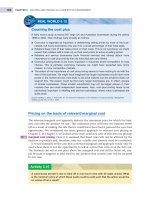
The learning-curve effect
Figure 7.10
Each time a particular task is performed, people become quicker at it. This learning-curve effect
becomes less and less significant until, after the task has been performed a number of times,
no further learning occurs.
M07_ATRI3622_06_SE_C07.QXD 5/29/09 10:38 AM Page 246

At this point, the point where the curve in Figure 7.10 becomes horizontal (the bottom
right of the graph), the learning-curve effect will have been eliminated and a steady,

long-term standard time for the activity will have been established.
The learning-curve effect seems to have little to do with whether workers are skilled
or unskilled; if they are unfamiliar with the task, the learning-curve effect will arise.
Practical experience shows that learning curves show remarkable regularity and, there-
fore, predictability from one activity to another.
The learning curve effect applies equally well to activities involved with providing
a service (such as dealing with an insurance claim, in an insurance business) as to
manufacturing-type activities (for example, upholstering an armchair by hand, in a
furniture-making business).
Clearly, the learning-curve effect must be taken into account when setting stand-
ards, and when interpreting any adverse labour efficiency variances, where a new pro-
cess and/or new staff are involved.
We have seen that standards can play a valuable role in performance evaluation and
control. However, standards that relate to costs, usages, selling prices and so on can
also be used for other purposes. In particular, they can be used to determine the cost
of inventories and work in progress for income-measurement purposes, and the cost of
items for use in pricing decisions.
Real World 7.7 provides some information on the use of standards in practice.
Other uses for standard costing
SOME PROBLEMS . . .
247
Although standards and variances may be useful for decision-making purposes, they
have limited application. Many business and commercial activities do not have direct
relationships between inputs and outputs as is the case with, say, the number of direct
labour hours worked and the number of products manufactured. Many expenses of
Some problems . . .
REAL WORLD 7.7
Standards in practice
The survey by Drury and others showed that respondent businesses found standards to
be useful for the following purposes:

Percentage of respondents
Cost control and performance evaluation 72
Valuing inventories and work in progress 80
Deducing costs for decision-making purposes 62
To help in constructing budgets 69
Source: Drury, C., Braund, S., Osborne, P. and Tayles, M., A Survey of Management Accounting Practices in UK Manufacturing
Companies, Chartered Association of Certified Accountants, 1993.
M07_ATRI3622_06_SE_C07.QXD 5/29/09 10:38 AM Page 247

modern business are in areas such as human resource development and advertising,
where the expense is discretionary and there is no direct link to the level of output.
There are also potential problems when applying standard costing techniques. These
include the following:
1 Standards can quickly become out of date as a result of both changes in the pro-
duction process and price changes. Standards should, therefore, be frequently mon-
itored and updated where necessary. Although this can be costly, it is essential if
standards are to be effective for control purposes. When standards become outdated,
performance can be adversely affected. For example, a human resources manager
who recognises that it is impossible to meet targets on rates of pay for labour,
because of general labour cost rises, may have less incentive to minimise costs.
2 Factors over which a particular manager has no control may affect a variance for
which that manager is held accountable. When assessing the manager’s perform-
ance, these uncontrollable factors should be taken into account but there is always
a risk that they will not.
3 In practice, creating clear lines of demarcation between the areas of responsibility of
various managers may be difficult. In this case, one of the prerequisites of effective
standard costing is lost.
4 Once a standard has been met, there is no incentive for employees to improve the
quality or quantity of output further. There are usually no additional rewards for
doing so; only additional work. Indeed, employees may have a disincentive for

exceeding a standard as it may then be viewed by managers as too loose and there-
fore in need of tightening. However, simply achieving a standard, and no more, may
not be enough in highly competitive and fast-changing markets. To compete effec-
tively, a business may need to strive for continuous improvement, and standard
costing techniques may impede this process.
5 Standard costing may create incentives for managers and employees to act in unde-
sirable ways. It may, for example, encourage the build up of excess inventories, lead-
ing to significant storage and financing costs. This problem can arise where there are
opportunities for discounts on bulk purchases of materials, which the purchasing
manager then exploits to achieve a favourable direct materials price variance. One
way to avoid this problem might be to impose limits on the level of inventories held.
A final example of the perverse incentives created by standard costing relates to
labour efficiency variances. Where these variances are calculated for individual
employees, and form the basis for their rewards, there is little incentive for them to
CHAPTER 7 ACCOUNTING FOR CONTROL
248
Can you think of another example of how a manager may achieve a favourable direct
materials price variance but in doing so would create problems for a business?
A manager may buy cheaper, but lower quality, materials. Although this may lead to a
favourable price variance, it may also lead to additional inspection and reworking costs,
and perhaps lost sales.
To avoid this problem, the manager may be required to buy material of a particular qual-
ity or from particular sources.
Activity 7.19
M07_ATRI3622_06_SE_C07.QXD 5/29/09 10:38 AM Page 248

work co-operatively. However, co-operative working may be in the best interests of the
business. To avoid this problem, some businesses calculate labour efficiency variances
for groups of employees rather than individual employees. This, however, creates the
risk that some individuals will become ‘free riders’ and will rely on the more consci-

entious employees to carry the load.
The traditional standard costing approach was developed during an era when business
operations were characterised by few product lines, long production runs and heavy
reliance on direct labour. More recently, the increasingly competitive environment
and the onward march of technology have changed the business landscape. Now,
many business operations are characterised by a wide range of different products,
shorter product life cycles (leading to shorter production runs) and automated pro-
duction processes. The effect of these changes has resulted in
l More frequent development of standards to deal with frequent changes to the pro-
duct range.
l A change in the focus for control. Where manufacturing systems are automated, for
example, direct labour becomes less important than direct materials.
l A decline in the importance of monitoring from cost and usage variances. Where
manufacturing systems are automated, deviations from standards relating to costs
and usage become less frequent and less significant.
Thus, where a business has highly automated production systems, traditional stand-
ard costing, with its emphasis on costs and usage, is likely to take on less importance.
Other elements of the production process such as quality, production levels, product
cycle times, delivery times and the need for continuous improvement become the
focus of attention. This does not mean, however, that a standards-based approach is
not useful for the new manufacturing environment. It can still provide valuable con-
trol information and there is no reason why standard costing systems cannot be
redesigned to reflect a concern for some of the elements mentioned earlier. Never-
theless, other measures, including non-financial ones, may help to augment the infor-
mation provided by the standard costing system. We shall consider this issue in more
detail in Chapter 10.
Real World 7.8 indicates that, despite the problems mentioned above, standard cost-
ing is used by businesses. However, the extent to which particular standard costing
variances are calculated and considered appears to vary.
The new business environment

THE NEW BUSINESS ENVIRONMENT
249
How might the business try to eliminate the ‘free-rider’ problem just mentioned?
One way would be to carry out an evaluation, perhaps by the group members themselves,
of individual contributions to group output, as well as evaluating group output as a whole.
Activity 7.20
M07_ATRI3622_06_SE_C07.QXD 5/29/09 10:38 AM Page 249

CHAPTER 7 ACCOUNTING FOR CONTROL
250
REAL WORLD 7.8
Standard practice
A study was carried out involving interviews with senior financial managers of businesses.
Standard costing was used by 30 of the businesses in the study, which represented most
of the businesses that might be expected to do so. The popularity among these busi-
nesses of standards for each of the main cost items is set out in Figure 7.11.
Despite the universal use of materials standards, the study found that four businesses
calculated the total direct materials variance only and that only two-thirds of businesses
calculated both the direct materials price and usage variances. For labour standards, the
variance analysis is even less complete. The study found that 15 businesses calculated
the total direct labour variance only and only one-third of businesses calculated both the
direct labour and efficiency variances. It seems, therefore, that standard costing was not
extensively employed by the businesses.
Source: Figure based on information in Dugdale, D., Jones, C. and Green, S., Contemporary Management Accounting Practices in
UK Manufacturing, Elsevier, 2006.
The popularity of standards in practice
Figure 7.11
Standards for materials were used by all businesses in the survey, and standards for
labour were used by nearly all businesses.
The main points of this chapter may be summarised as follows:

Controlling through budgets
l Budgets act as a system of both feedback and feedforward control.
l To exercise control, budgets can be flexed to match actual volume of output.
Variance analysis
l Variances may be favourable or adverse according to whether they result in an
increase to, or decrease from, the budgeted profit figure.
SUMMARY
M07_ATRI3622_06_SE_C07.QXD 5/29/09 10:38 AM Page 250

l Budgeted profit plus all favourable variances less all adverse variances equals actual
profit.
l Commonly calculated variances:
– Sales volume variance = difference between the original and flexed budget profit
figures.
– Sales price variance = difference between actual sales revenue and actual volume
at the standard sales price.
– Total direct materials variance = difference between the actual direct materials
cost and the direct materials cost according to the flexed budget.
– Direct materials usage variance = difference between actual usage and budgeted
usage, for the actual volume of output, multiplied by the standard materials
cost.
– Direct materials price variance = difference between the actual materials cost and
the actual usage multiplied by the standard materials cost.
– Total direct labour variance = The difference between the actual direct labour cost
and the direct labour cost according to the flexed budget.
– Direct labour efficiency variance = difference between actual labour time and
budgeted time, for the actual volume of output, multiplied by the standard labour
rate.
– Direct labour rate variance = difference between the actual labour cost and the
actual labour time multiplied by the standard labour rate.

– Fixed overhead spending variance = difference between the actual and budgeted
spending on fixed overheads.
l Significant and/or persistent variances should normally be investigated to establish
their cause. However, the costs and benefits of investigating variances must be
considered.
l Trading off favourable variances against linked adverse variances should not be auto-
matically acceptable.
l Not all activities can usefully be controlled through traditional variance analysis.
Effective budgetary control
l Good budgetary control requires establishing systems and routines to ensure such
things as a clear distinction between individual managers’ areas of responsibil-
ity; prompt, frequent and relevant variance reporting; and senior management
commitment.
l There are behavioural aspects of control relating to management style, participation
in budget setting and the failure to meet budget targets that should be taken into
account by senior managers.
Standard costing
l Standards = budgeted physical quantities and financial values for one unit of inputs
and outputs.
l There are two types of standards: ideal standards and practical standards.
l Information necessary for developing standards can be gathered by analysing the
task or by using past data.
l There tends to be a learning-curve effect: routine tasks are performed more quickly
with experience.
l Standards are useful in providing data for income measurement and pricing
decisions.
l Standards have their limitations, particularly in modern manufacturing environ-
ments, however, they are still widely used.
SUMMARY
251

M07_ATRI3622_06_SE_C07.QXD 5/29/09 10:38 AM Page 251

1 Hopwood, A. G., ‘An empirical study of the role of accounting data in performance evalua-
tion’, Empirical Research in Accounting, a supplement to the Journal of Accounting Research, 1972,
pp. 156–82.
If you would like to explore the topics covered in this chapter in more depth, we recommend the
following books:
Atkinson, A., Kaplan, R., Young, S. M. and Matsumura, E., Management Accounting, 5th edn,
Prentice Hall, 2007, chapter 12.
Drury C., Management and Cost Accounting, 7th edn, Thomson Learning Business Press, 2008,
chapters 16–18.
Bhimani, A., Horngren, C., Datar, S. and Foster, G., Management and Cost Accounting, 4th edn, FT
Prentice Hall 2008, chapters 14–16.
Hilton, R., Managerial Accounting, 6th edn, McGraw-Hill Irwin, 2005, chapter 10.
Further reading
References
CHAPTER 7 ACCOUNTING FOR CONTROL
252
Feedback control p. 219
Feedforward control p. 219
Flexing the budget p. 221
Flexible budget p. 222
Sales volume variance p. 223
Adverse variance p. 223
Favourable variance p. 223
Variance p. 223
Sales price variance p. 225
Total direct materials variance p. 225
Direct materials usage variance
p. 225

Direct materials price variance
p. 226
Total direct labour variance p. 227
Direct labour efficiency variance
p. 227
Direct labour rate variance p. 227
Fixed overhead spending variance
p. 228
Non-operating profit variances
p. 235
Compensating variances p. 238
Budgetary control p. 239
Behavioural aspects of budgetary
control p. 242
Standard quantities and costs p. 244
Ideal standards p. 245
Practical standards p. 245
Learning curve p. 246
Key terms
‘
M07_ATRI3622_06_SE_C07.QXD 5/29/09 10:38 AM Page 252

Answers to these questions can be found in Appendix D at the back of the book.
Explain what is meant by feedforward control and distinguish it from feedback control.
What is meant by a variance? What is the point in analysing variances?
What is the point in flexing the budget in the context of variance analysis? Does flexing imply that
differences between budget and actual in the volume of output are ignored in variance analysis?
Should all variances be investigated to find their cause? Explain your answer.
7.4
7.3

7.2
7.1
Exercises 7.4 to 7.8 are more advanced than 7.1 to 7.3. Those with coloured numbers have
answers in Appendix D at the back of the book. If you wish to try more exercises, visit the
students’ side of the Companion Website at www.pearsoned.co.uk/atrillmclaney.
You have recently overheard the following remarks:
(a)
‘A favourable direct labour rate variance can only be caused by staff working more effi-
ciently than budgeted.’
(b) ‘Selling more units than budgeted, because the units were sold at less than standard price,
automatically leads to a favourable sales volume variance.’
(c) ‘Using below-standard materials will tend to lead to adverse materials usage variances but
cannot affect labour variances.’
(d) ‘Higher-than-budgeted sales could not possibly affect the labour rate variance.’
(e) ‘An adverse sales price variance can only arise from selling a product at less than standard
price.’
Required:
Critically assess these remarks, explaining any technical terms.
Pilot Ltd makes a standard product, which is budgeted to sell at £5.00 a unit. It is made by tak-
ing a budgeted 0.5 kg of material, budgeted to cost £3.00 a kilogram, and working on it by hand
by an employee, paid a budgeted £10.00 an hour, for a budgeted 7
1
/2 minutes. Monthly fixed
overheads are budgeted at £6,000. The output for March was budgeted at 5,000 units.
The actual results for March were as follows:
£
Sales revenue (5,400 units) 26,460
Materials (2,830 kg) (8,770)
Labour (650 hours) (6,885)
Fixed overheads (6,350)

Actual operating profit 4,455
No inventories existed at the start or end of March.
Required:
(a) Deduce the budgeted profit for March and reconcile it with the actual profit in as much detail
as the information provided will allow.
(b) State which manager should be held accountable, in the first instance, for each variance
calculated.
7.2
7.1
EXERCISES
253
REVIEW QUESTIONS
EXERCISES
M07_ATRI3622_06_SE_C07.QXD 5/29/09 10:38 AM Page 253

Antonio plc makes Product X, the standard costs of which are:
£
Sales revenue 31
Direct labour (1 hour) (11)
Direct materials (1 kg) (10)
Fixed overheads (3)
Standard profit 7
The budgeted output for March was 1,000 units of Product X; the actual output was 1,100 units,
which was sold for £34,950. There were no inventories at the start or end of March.
The actual production costs were:
£
Direct labour (1,075 hours) 12,210
Direct materials (1,170 kg) 11,630
Fixed overheads 3,200
Required:

Calculate the variances for March as fully as you are able from the available information, and
use them to reconcile the budgeted and actual profit figures.
You have recently overheard the following remarks:
(a) ‘When calculating variances, we in effect ignore differences of volume of output, between
original budget and actual, by flexing the budget. If there were a volume difference, it is
water under the bridge by the time that the variances come to be calculated.’
(b) ‘It is very valuable to calculate variances because they will tell you what went wrong.’
(c) ‘All variances should be investigated to find their cause.’
(d) ‘Research evidence shows that the more demanding the target, the more motivated the
manager.’
(e) ‘Most businesses do not have feedforward controls of any type, just feedback controls
through budgets.’
Required:
Critically assess these remarks, explaining any technical terms.
Bradley-Allen Ltd makes one standard product. Its budgeted operating statement for May is as
follows:
££
Sales (volume and revenue): 800 units 64,000
Direct materials: Type A (12,000)
Type B (16,000)
Direct labour: skilled (4,000)
unskilled (10,000)
Overheads: (all fixed) (12,000)
(54,000)
Budgeted operating profit 10,000
The standard costs were as follows:
l Direct materials: Type A £50/kg
Type B £20/m
l Direct labour: skilled £10/hour
unskilled £8/hour

7.5
7.4
7.3
CHAPTER 7 ACCOUNTING FOR CONTROL
254
M07_ATRI3622_06_SE_C07.QXD 5/29/09 10:38 AM Page 254

During May, the following occurred:
(1) 950 units were sold for a total of £73,000.
(2) 310 kilos (costing £15,200) of Type A material were used in production.
(3) 920 metres (costing £18,900) of Type B material were used in production.
(4) Skilled workers were paid £4,628 for 445 hours.
(5) Unskilled workers were paid £11,275 for 1,375 hours.
(6) Fixed overheads cost £11,960.
There were no inventories of finished production or of work in progress at either the beginning
or end of May.
Required:
(a) Prepare a statement that reconciles the budgeted to the actual profit of the business for
May, through variances. Your statement should analyse the difference between the two
profit figures in as much detail as you are able.
(b) Explain how the statement in (a) might be helpful to managers.
Mowbray Ltd makes and sells one product, the standard costs of which are as follows:
£
Direct materials (3 kg at £2.50/kg) (7.50)
Direct labour (15 minutes at £9.00/hr) (2.25)
Fixed overheads (3.60)
(13.35)
Selling price 20.00
Standard profit margin 6.65
The monthly production and sales are planned to be 1,200 units.

The actual results for May were as follows:
£
Sales revenue 18,000
Direct materials (7,400) (2,800 kg)
Direct labour (2,300) (255 hr)
Fixed overheads (4,100)
Operating profit 4,200
There were no inventories at the start or end of May. As a result of poor sales demand during
May, the business reduced the price of all sales by 10 per cent.
Required:
Calculate the budgeted profit for May and reconcile it to the actual profit through variances,
going into as much detail as is possible from the information available.
Varne Chemprocessors is a business that specialises in plastics. It uses a standard costing sys-
tem to monitor and report its purchases and usage of materials. During the most recent month,
accounting period six, the purchase and usage of chemical UK194 were as follows:
Purchases/usage: 28,100 litres
Total price: £51,704
Because of fire risk and the danger to health, no inventories are held by the business.
UK194 is used solely in the manufacture of a product called Varnelyne. The standard cost
specification shows that, for the production of 5,000 litres of Varnelyne, 200 litres of UK194
are needed at a total standard cost of £392. During period six, 637,500 litres of Varnelyne were
produced.
7.7
7.6
EXERCISES
255
M07_ATRI3622_06_SE_C07.QXD 5/29/09 10:38 AM Page 255

Price variances, over recent periods, for two other raw materials used by the business are as
follows:

Period UK500 UK800
££
1 301 F 298 F
2 251 A 203 F
3 102 F 52 A
4 202 A 98 A
5 153 F 150 A
6 103 A 201 A
where F = favourable variance and A = adverse variance.
Required:
(a) Calculate the price and usage variances for UK194 for period six.
(b) The following comment was made by the production manager:
‘I knew at the beginning of period six that UK194 would be cheaper than the standard cost
specification, so I used rather more of it than normal; this saved £4,900 on other chemicals.’
What changes do you need to make in your analysis for (a) as a result of this comment?
(c) Calculate for both UK500 and UK800, the cumulative price variances and comment briefly
on the results.
Brive plc has the following standards for its only product:
Selling price: £110/unit
Direct labour: 1 hour at £10.50/hour
Direct material: 3 kg at £14.00/kg
Fixed overheads: £27.00/unit, based on a budgeted output of 800 units/month
During May, there was an actual output of 850 units and the operating statement for the
month was as follows:
£
Sales revenue 92,930
Direct labour (890 hours) (9,665)
Direct materials (2,410 kg) (33,258)
Fixed overheads (21,365)
Operating profit 28,642

There were no inventories of any description at the beginning or end of May.
Required:
Prepare the original budget and a budget flexed to the actual volume. Use these to compare the
budgeted and actual profits of the business for the month, going into as much detail with your
analysis as the information given will allow.
7.8
CHAPTER 7 ACCOUNTING FOR CONTROL
256
M07_ATRI3622_06_SE_C07.QXD 5/29/09 10:38 AM Page 256

Making capital investment
decisions
LEARNING OUTCOMES
This chapter looks at how proposed investments in new plant, machinery, buildings
and other long-term assets should be evaluated. This is a very important area for
businesses; expensive and far-reaching consequences can flow from bad
investment decisions.
We shall also consider the problem of risk and how this may be taken into
account when evaluating investment proposals. Finally, we shall discuss the ways
that managers can oversee capital investment projects and how control may be
exercised throughout the life of a project.
INTRODUCTION
8
When you have completed this chapter, you should be able to:
l Explain the nature and importance of investment decision making.
l Identify the four main investment appraisal methods found in practice.
l Discuss the strengths and weaknesses of various techniques for dealing with
risk in investment appraisal.
l Explain the methods used to monitor and control investment projects.
M08_ATRI3622_06_SE_C08.QXD 5/29/09 3:31 PM Page 257

The essential feature of investment decisions is time. Investment involves making an
outlay of something of economic value, usually cash, at one point in time, which is
expected to yield economic benefits to the investor at some other point in time.
Usually, the outlay precedes the benefits. Also, the outlay is typically one large amount
and the benefits arrive as a series of smaller amounts over a fairly protracted period.
Investment decisions tend to be of profound importance to the business because
l Large amounts of resources are often involved. Many investments made by businesses
involve laying out a significant proportion of their total resources (see Real World 8.2).
If mistakes are made with the decision, the effects on the businesses could be
significant, if not catastrophic.
l It is often difficult and/or expensive to bail out of an investment once it has been under-
taken. It is often the case that investments made by a business are specific to its
needs. For example, a hotel business may invest in a new, custom-designed hotel
complex. The specialist nature of this complex will probably lead to its having a
rather limited second-hand value to another potential user with different needs. If
the business found, after having made the investment, that room occupancy rates
were not as buoyant as was planned, the only possible course of action might be to
close down and sell the complex. This would probably mean that much less could
be recouped from the investment than it had originally cost, particularly if the costs
of design are included as part of the cost, as they logically should be.
Real World 8.1 gives an illustration of a major investment by a well-known business
operating in the UK.
The nature of investment decisions
CHAPTER 8 MAKING CAPITAL INVESTMENT DECISIONS
258
REAL WORLD 8.1
Brittany Ferries launches an investment
Brittany Ferries, the cross-Channel ferry operator, recently had a new ship built, to be
named Armorique. The ship cost the business about A81m and is used on the Plymouth

to Roscoff route as from Spring 2009. Although Brittany Ferries is a substantial business,
this level of expenditure was significant. Clearly, the business believed that acquisition of
the new ship would be profitable for it, but how would it have reached this conclusion?
Presumably the anticipated future cash flows from passengers and freight operators will
have been major inputs to the decision. The ship was specifically designed for Brittany
Ferries, so it would be difficult for the business to recoup a large proportion of its A81m
should these projected cash flows not materialise.
Source: ‘New A81m passenger cruise-ferry to be named “Armorique” ’, www.brittany-ferries.co.uk.
The issues raised by Brittany Ferries’ investment will be the main subject of this chapter.
Real World 8.2 indicates the level of annual net investment for a number of ran-
domly selected, well-known UK businesses. It can be seen that the scale of investment
varies from one business to another. (It also tends to vary from one year to the next for
a particular business.) In nearly all of these businesses the scale of investment is very
significant.
M08_ATRI3622_06_SE_C08.QXD 5/29/09 3:31 PM Page 258

Real World 8.2 is limited to considering the non-current asset investment, but most
non-current asset investment also requires a level of current asset investment to sup-
port it (additional inventories, for example), meaning that the real scale of investment
is even greater, typically considerably so, than indicated above.
INVESTMENT APPRAISAL METHODS
259
REAL WORLD 8.2
The scale of investment by UK businesses
Expenditure on additional non-current
assets as a percentage of:
Annual sales revenue End-of-year
non-current assets
BT plc (telecommunications) 15.9 17.5
Babcock International Group plc 6.8 20.6

(support services)
Tesco plc (supermarkets) 5.5 11.6
J D Wetherspoon plc (pub operator) 12.5 9.0
Marks and Spencer plc (stores) 7.6 14.4
National Grid plc (utilities) 48.0 19.8
J. Sainsbury plc (supermarkets) 4.0 8.9
First Group plc (passenger transport) 5.7 13.1
Source: Annual reports of the businesses concerned for the financial year ending in 2007.
When managers are making decisions involving capital investments, what should the
decisions seek to achieve?
Investment decisions must be consistent with the objectives of the particular business. For
a private sector business, maximising the wealth of the owners (shareholders) is usually
assumed to be the key financial objective.
Activity 8.1
Given the importance of investment decisions, it is essential that there is proper
screening of investment proposals. An important part of this screening process is to
ensure that the business uses appropriate methods of evaluation.
Research shows that there are basically four methods used in practice by businesses
throughout the world to evaluate investment opportunities. They are:
l accounting rate of return (ARR)
l payback period (PP)
l net present value (NPV)
l internal rate of return (IRR).
Investment appraisal methods
M08_ATRI3622_06_SE_C08.QXD 5/29/09 3:31 PM Page 259

It is possible to find businesses that use variants of these four methods. It is also pos-
sible to find businesses, particularly smaller ones, that do not use any formal appraisal
method but rely instead on the ‘gut feeling’ of their managers. Most businesses, however,
seem to use one (or more) of these four methods.

We are going to assess the effectiveness of each of these methods and we shall see
that only one of them (NPV) is a wholly logical approach. The other three all have
flaws. We shall also see how popular these four methods seem to be in practice.
To help us to examine each of the methods, it might be useful to consider how each
of them would cope with a particular investment opportunity. Let us consider the
following example.
CHAPTER 8 MAKING CAPITAL INVESTMENT DECISIONS
260
Billingsgate Battery Company has carried out some research that shows that the
business could provide a standard service that it has recently developed.
Provision of the service would require investment in a machine that would cost
£100,000, payable immediately. Sales of the service would take place throughout
the next five years. At the end of that time, it is estimated that the machine could
be sold for £20,000.
Inflows and outflows from sales of the service would be expected to be as
follows:
Time £000
Immediately Cost of machine (100)
1 year’s time Operating profit before depreciation 20
2 years’ time Operating profit before depreciation 40
3 years’ time Operating profit before depreciation 60
4 years’ time Operating profit before depreciation 60
5 years’ time Operating profit before depreciation 20
5 years’ time Disposal proceeds from the machine 20
Note that, broadly speaking, the operating profit before deducting depreciation
(that is, before non-cash items) equals the net amount of cash flowing into the
business. Apart from depreciation, all of this business’s expenses cause cash to
flow out of the business. Sales revenues lead to cash flowing in. If, for the time
being, we assume that inventories, trade receivables and trade payables remain
constant, operating profit before depreciation will equal the cash inflow.

To simplify matters, we shall assume that the cash from sales and for the
expenses of providing the service are received and paid, respectively, at the end of
each year. This is clearly unlikely to be true in real life. Money will have to be paid
to employees (for salaries and wages) on a weekly or a monthly basis. Customers
will pay within a month or two of buying the service. On the other hand, making
the assumption probably does not lead to a serious distortion. It is a simplifying
assumption that is often made in real life, and it will make things more straight-
forward for us now. We should be clear, however, that there is nothing about any
of the four methods that demands that this assumption is made.
Example 8.1
M08_ATRI3622_06_SE_C08.QXD 5/29/09 3:31 PM Page 260

ACCOUNTING RATE OF RETURN (ARR)
261
‘
Having set up the example, we shall now go on to consider how each of the
appraisal methods works.
The accounting rate of return (ARR) method takes the average accounting operating
profit that the investment will generate and expresses it as a percentage of the average
investment made over the life of the project. Thus:
We can see from the equation that, to calculate the ARR, we need to deduce two
pieces of information about the particular project:
l the annual average operating profit; and
l the average investment.
In our example, the average annual operating profit before depreciation over the five
years is £40,000 (that is, £000(20 + 40 + 60 + 60 + 20)/5). Assuming ‘straight-line’ depre-
ciation (that is, equal annual amounts), the annual depreciation charge will be £16,000
(that is, £(100,000 − 20,000)/5). Thus the average annual operating profit after depreci-
ation is £24,000 (that is, £40,000 − £16,000).
The average investment over the five years can be calculated as follows:

Average investment =
=
= £60,000
Thus, the ARR of the investment is
ARR =×100% = 40%
Users of ARR should apply the following decision rules:
l For any project to be acceptable it must achieve a target ARR as a minimum.
l Where there are competing projects that all seem capable of exceeding this
minimum rate (that is, where the business must choose between more than one
project), the one with the higher (or highest) ARR would normally be selected.
To decide whether the 40 per cent return is acceptable, we need to compare this per-
centage return with the minimum rate required by the business.
£24,000
£60,000
£100,000 + £20,000
2
Cost of machine + Disposal value
2
Average annual operating profit
ARR
==
Average investment to earn that profit
××
100%
Accounting rate of return (ARR)
M08_ATRI3622_06_SE_C08.QXD 5/29/09 3:31 PM Page 261

ARR and ROCE
We should note that ARR and the return on capital employed (ROCE) ratio take the
same approach to performance measurement, in that they both relate accounting

profit to the cost of the assets invested to generate that profit. ROCE is a popular means
of assessing the performance of a business, as a whole, after it has performed. ARR is an
approach that assesses the potential performance of a particular investment, taking the
same approach as ROCE, but before it has performed.
As we have just seen, managers using ARR will require that any investment under-
taken should achieve a target ARR as a minimum. Perhaps the minimum target ROCE
CHAPTER 8 MAKING CAPITAL INVESTMENT DECISIONS
262
Chaotic Industries is considering an investment in a fleet of ten delivery vans to take its
products to customers. The vans will cost £15,000 each to buy, payable immediately.
The annual running costs are expected to total £20,000 for each van (including the
driver’s salary). The vans are expected to operate successfully for six years, at the end
of which period they will all have to be sold, with disposal proceeds expected to be
about £3,000 a van. At present, the business uses a commercial carrier for all of its
deliveries. It is expected that this carrier will charge a total of £230,000 each year for
the next six years to undertake the deliveries.
What is the ARR of buying the vans? (Note that cost savings are as relevant a ben-
efit from an investment as are net cash inflows.)
The vans will save the business £30,000 a year (that is, £230,000 − (£20,000 × 10)), before
depreciation, in total. Thus, the inflows and outflows will be:
Time £000
Immediately Cost of vans (10 × £15,000) (150)
1 year’s time Net saving before depreciation 30
2 years’ time Net saving before depreciation 30
3 years’ time Net saving before depreciation 30
4 years’ time Net saving before depreciation 30
5 years’ time Net saving before depreciation 30
6 years’ time Net saving before depreciation 30
6 years’ time Disposal proceeds from the vans (10 × £3,000) 30
The total annual depreciation expense (assuming a straight-line method) will be

£20,000 (that is, (£150,000 − £30,000)/6). Thus, the average annual saving, after depreci-
ation, is £10,000 (that is, £30,000 − £20,000).
The average investment will be
Average investment ==£90,000
and the ARR of the investment is
ARR =×100% = 11.1%
£10,000
£90,000
£150,000 + £30,000
2
Activity 8.2
M08_ATRI3622_06_SE_C08.QXD 5/29/09 3:31 PM Page 262

would be based on the rate that previous investments had actually achieved (as mea-
sured by ROCE). Perhaps it would be the industry-average ROCE.
Since private sector businesses are normally seeking to increase the wealth of their
owners, ARR may seem to be a sound method of appraising investment opportunities.
Operating profit can be seen as a net increase in wealth over a period, and relating it
to the size of investment made to achieve it seems a logical approach.
ARR is said to have a number of advantages as a method of investment appraisal. It
was mentioned earlier that ROCE seems to be a widely used measure of business per-
formance. Shareholders seem to use this ratio to evaluate management performance,
and sometimes the financial objective of a business will be expressed in terms of a tar-
get ROCE. It therefore seems sensible to use a method of investment appraisal that is
consistent with this overall approach to measuring business performance. It also gives
the result expressed as a percentage. It seems that many managers feel comfortable
using measures expressed in percentage terms.
Problems with ARR
ACCOUNTING RATE OF RETURN (ARR)
263

ARR suffers from a very major defect as a means of assessing investment opportu-
nities. Can you reason out what this is? Consider the three competing projects whose
profits are shown below. All three involve investment in a machine that is expected to
have no residual value at the end of the five years. Note that all of the projects have the
same total operating profits over the five years.
Time Project A Project B Project C
£000 £000 £000
Immediately Cost of machine (160) (160) (160)
1 year’s time Operating profit after depreciation 20 10 160
2 years’ time Operating profit after depreciation 40 10 10
3 years’ time Operating profit after depreciation 60 10 10
4 years’ time Operating profit after depreciation 60 10 10
5 years’ time Operating profit after depreciation 20 160 10
(Hint: The defect is not concerned with the ability of the decision maker to forecast
future events, although this too can be a problem. Try to remember the essential feature
of investment decisions, which we identified at the beginning of this chapter.)
The problem with ARR is that it almost completely ignores the time factor. In this example,
exactly the same ARR would have been computed for each of the three projects.
Since the same total operating profit over the five years (£200,000) arises in all three of
these projects, and the average investment in each project is £80,000 (that is, £160,000/2),
this means that each case will give rise to the same ARR of 50 per cent (that is, £40,000/
£80,000).
Activity 8.3
Given a financial objective of maximising the wealth of the owners of the business,
any rational decision maker faced with a choice between the three projects set out in
Activity 8.3 would strongly prefer Project C. This is because most of the benefits from
M08_ATRI3622_06_SE_C08.QXD 5/29/09 3:31 PM Page 263

the investment arise within twelve months of investing the £160,000 to establish
the project. Project A would rank second and Project B would come a poor third.

Any appraisal technique that is not capable of distinguishing between these three
situations is seriously flawed. We shall look at why timing is so important later in the
chapter.
There are further problems associated with the use of ARR. One of these problems
concerns the approach taken to derive the average investment in a project.
Example 8.2 illustrates the daft result that ARR can produce.
CHAPTER 8 MAKING CAPITAL INVESTMENT DECISIONS
264
George put forward an investment proposal to his boss. The business uses ARR to
assess investment proposals using a minimum ‘hurdle’ rate of 27 per cent. Details
of the proposal were as follows:
Cost of equipment £200,000
Estimated residual value of equipment £40,000
Average annual operating profit
before depreciation £48,000
Estimated life of project 10 years
Annual straight-line depreciation charge £16,000 (that is, (£200,000 − £40,000)/10)
The ARR of the project will be:
ARR =×100% = 26.7%
The boss rejected George’s proposal because it failed to achieve an ARR of at least
27 per cent. Although George was disappointed, he realised that there was still hope.
In fact, all that the business had to do was to give away the piece of equipment at
the end of its useful life rather than to sell it. The residual value of the equipment
then became zero and the annual depreciation charge became ([£200,000 − £0]/10)
= £20,000 a year. The revised ARR calculation was then as follows:
ARR =×100% = 28%
48,000 − 20,000
(200,000 + 0)/2
48,000 − 16,000
(200,000 + 40,000)/2

Example 8.2
ARR is based on the use of accounting profit. When measuring performance over
the whole life of a project, however, it is cash flows rather than accounting profits that
are important. Cash is the ultimate measure of the economic wealth generated by an
investment. This is because it is cash that is used to acquire resources and for distribu-
tion to owners. Accounting profit, on the other hand is more appropriate for reporting
achievement on a periodic basis. It is a useful measure of productive effort for a rela-
tively short period, such as a year or half year. It is really a question of ‘horses for
courses’. Accounting profit is fine for measuring performance over short periods, but
cash is the appropriate measure when considering the performance over the life of a
project.
The ARR method can also create problems when considering competing investments
of different size.
M08_ATRI3622_06_SE_C08.QXD 5/29/09 3:31 PM Page 264

Real World 8.3 illustrates how using percentage measures can lead to confusion.
PAYBACK PERIOD (PP)
265
‘
Sinclair Wholesalers plc is currently considering opening a new sales outlet in
Coventry. Two possible sites have been identified for the new outlet. Site A has an
area of 30,000 sq m. It will require an average investment of £6m, and will produce an
average operating profit of £600,000 a year. Site B has an area of 20,000 sq m. It will
require an average investment of £4m, and will produce an average operating profit of
£500,000 a year.
What is the ARR of each investment opportunity? Which site would you select,
and why?
The ARR of Site A is £600,000/£6m = 10 per cent. The ARR of Site B is £500,000/£4m
= 12.5 per cent. Thus, Site B has the higher ARR. However, in terms of the absolute
operating profit generated, Site A is the more attractive. If the ultimate objective is to

increase the wealth of the shareholders of Sinclair Wholesalers plc, it might be better to
choose Site A even though the percentage return is lower. It is the absolute size of the
return rather than the relative (percentage) size that is important. This is a general problem
of using comparative measures, such as percentages, when the objective is measured in
absolute ones, like an amount of money. If businesses were seeking through their invest-
ments to generate a percentage rate of return on investment, ARR would be more helpful.
The problem is that most businesses seek to achieve increases in their absolute wealth
(measured in pounds, euros, dollars and so on) through their investment decisions.
Activity 8.4
REAL WORLD 8.3
Increasing road capacity by sleight of hand
During the 1970s, the Mexican government wanted to increase the capacity of a major
four-lane road. It came up with the idea of repainting the lane markings so that there were
six narrower lanes occupying the same space as four wider ones had previously done.
This increased the capacity of the road by 50 per cent (that is,
2
/4 × 100). A tragic outcome
of the narrower lanes was an increase in deaths from road accidents. A year later the
Mexican government had the six narrower lanes changed back to the original four wider
ones. This reduced the capacity of the road by 33 per cent (that is,
2
/6 × 100). The Mexican
government reported that, overall, it had increased the capacity of the road by 17 per cent
(that is, 50% − 33%), despite the fact that its real capacity was identical to that which it
had been originally. The confusion arose because each of the two percentages (50 per cent
and 33 per cent) is based on different bases (four and six).
Source: Gigerenzer, G., Reckoning with Risk, Penguin, 2002.
The payback period (PP) is the length of time it takes for an initial investment to be
repaid out of the net cash inflows from a project. Since it takes time into account, the
PP method seems to go some way towards overcoming the timing problem of ARR – or

at first glance it does.
Payback period (PP)
M08_ATRI3622_06_SE_C08.QXD 5/29/09 3:31 PM Page 265

CHAPTER 8 MAKING CAPITAL INVESTMENT DECISIONS
266
It might be useful to consider PP in the context of the Billingsgate Battery example.
We should recall that essentially the project’s cash flows are:
Time £000
Immediately Cost of machine (100)
1 year’s time Operating profit before depreciation 20
2 years’ time Operating profit before depreciation 40
3 years’ time Operating profit before depreciation 60
4 years’ time Operating profit before depreciation 60
5 years’ time Operating profit before depreciation 20
5 years’ time Disposal proceeds 20
Note that all of these figures are amounts of cash to be paid or received (we saw
earlier that operating profit before depreciation is a rough measure of the cash flows
from the project).
As the payback period is the length of time it takes for the initial investment to be
repaid out of the net cash inflows, it will be three years before the £100,000 outlay is
covered by the inflows. This is still assuming that the cash flows occur at year ends. The
payback period can be derived by calculating the cumulative cash flows as follows:
Time Net cash Cumulative
flows cash flows
£000 £000
Immediately Cost of machine (100) (100)
1 year’s time Operating profit before depreciation 20 (80) (−100 + 20)
2 years’ time Operating profit before depreciation 40 (40) (−80 + 40)
3 years’ time Operating profit before depreciation 60 20 (−40 + 60)

4 years’ time Operating profit before depreciation 60 80 (20 + 60)
5 years’ time Operating profit before depreciation 20 100 (80 + 20)
5 years’ time Disposal proceeds 20 120 (100 + 20)
We can see that the cumulative cash flows become positive at the end of the third
year. Had we assumed that the cash flows arise evenly over the year, the precise pay-
back period would be
2 years + (
40
/60) years = 2
2
/3 years
where 40 represents the cash flow still required at the beginning of the third year to
repay the initial outlay, and 60 is the projected cash flow during the third year.
We must now ask how to decide whether three years is an acceptable payback period.
The decision rule for using PP is:
l For a project to be acceptable it would need to have a payback period shorter than
a maximum payback period set by the business.
l If there were two (or more) competing projects whose payback periods were all
shorter than the maximum payback period requirement, the project with the
shorter (or shortest) payback period should be selected.
If, for example, Billingsgate Battery had a maximum acceptable payback period of
four years, the project would be undertaken. A project with a longer payback period
than four years would not be acceptable.
M08_ATRI3622_06_SE_C08.QXD 5/29/09 3:31 PM Page 266