Hindawi Publishing Corporation EURASIP Journal on Wireless Communications and Networking Volume pdf

Hindawi Publishing Corporation
EURASIP Journal on Wireless Communications and Networking
Volume 2011, Article ID 263134, 16 pages
doi:10.1155/2011/263134
Research Ar ticle
Statistical Analysis of Multipath Clustering in
an Indoor Office Environment
Emmeric Tanghe,
1
Wout Joseph,
1, 2
Martine Li
´
enard,
2
Abdelmottaleb Nasr,
2
Paul Stefanut,
2
Luc Martens,
1
and Pierre Degauque
2
1
Department of Information Technology, Ghent University-IBBT, Gaston Crommenlaan 8 box 201, 9050 Ghent, Belgium
2
Gr oup TELICE, IEMN, University of Lille, Building P3, 59655 Villeneuve d’Ascq, France
Correspondence should be addressed to Emmeric Tanghe,
Received 12 August 2010; Revised 15 December 2010; Accepted 21 February 2011
Academic Editor: Nicolai Czink
Copyright © 2011 Emmeric Tanghe et al. This is an open access article distributed under the Creative Commons Attribution

License, which permits unrestricted use, distribution, and repr oduction in any medium, provided the original work is properly
cited.
A parametric directional-based MIMO channel model is presented which takes multipath clustering into acc ount. The directional
propagation path parameters include azimuth of arrival (AoA), azimuth of departure (AoD), delay, and power. MIMO
measurements are carried out in an indoor office environment using the virtual antenna array method with a vector network
analyzer. Propagation paths a re extracted using a joint 5D ESPRIT algorithm and are automatically clustered with the K-
power-means algorithm. This work focuses on the statistical treatment of the propagation parameters w ithin individual clusters
(intracluster statistics) a nd the change in these parameters from one cluster to another (intercluster statistics). Motivated choices
for the statistical distributions of the intr a cluster and intercluster parameters are made. To validate these choices, the parameters’
goodness of fit to the proposed distributions is verified using a number of powerful statistical hypothesis tests. Additionally,
parameter correlations are calculated and tested for their significance. Building on the concept of multipath clusters, this paper also
provides a new notation of the MIMO channel matrix (named FActorization into a BLock-diagonal Expression or FABLE)which
more visibly shows the clustered nature of propagation paths.
1. Introduction
To meet the ever-increasing requirements for reliable com-
munication with high throughput, novel wireless tech-
nologies have to be considered. A promising approach to
increase wireless capacity is to exploit the spatial structure
of wireless channels through multiple-input multiple-output
(MIMO) techniques. High-throughput MIMO specifica-
tions are already being included in wireless standards, most
notably IEEE 802.11n [1], IEEE 802.16e [2], and 3GPP Long-
Term Evolution (LTE) [3]. MIMO is one of the principal
technologies that will be used by 4G communication net-
works.
The potential benefits of implementing MIMO are
highly dependent on the characteristics of the propagation
environment. A lot of progress has been made in the
development of different types of MIMO channel models
for signal processing algorithm testing [4]. In recent years,

the geometr y-based stochastic type of channel models, first
proposed in [5], gains research interest. These kind of models
present a statistical distribution for the propagation path
parameters (e.g., direction of arrival, direction of departure,
delay, etc.), while also taking some geometry parameters
of the environment into account (e.g., the location of
scatterers). For the moment, most geometry-based stochastic
channel models use propagation path clusters in their
description. Clustering of propagation paths seems to occur
naturally in wave propagation and as an added benefit helps
to reduce the number of statistical parameters needed to
construct the model. Examples of geometry-based stochastic
channel models can be found in [6–9].
This work investigates the statistics of propagation path
parameters including directions of arrival and departure,
delay, and power in an indoor office environment. For this,
2 EURASIP Journal on Wireless Communications and Networking
MIMO channel sounding measurements with a virtual
antenna array are carried out on an office floor. Propa-
gation path parameters are extracted from measurement
data and are subsequently grouped into clusters using an
automatic clustering algorithm. Following, propagation path
parameters are split up into an intercluster part and an
intracluster part; the former is representative for the location
in propagation path parameter space of the cluster to which
the path belongs, while the latter is defined as the propaga-
tion path parameter’s deviation from the intercluster part.
Additionally, a new notational improvement of the wireless
channel matrix is proposed which makes the separation of
propagation path parameters into intercluster and intraclus-

ter parts more visible. This decomposition of the MIMO
channel matrix is named FActorization into a BLock-diagonal
Expression (FA BLE), because the decomposition includes a
block-diagonal form of the intracluster parameters.
Next, the intercluster and intracluster dynamics are mod-
elled statistically. Choices for the statistical distributions are
physically and statistically motivated; those types of distribu-
tions are chosen which in our opinion most accurately agree
with the underlying propagation physics and which match
the support of the propagation parameters (e.g., the von
Mises dist ribution for angular data). Distributional choices
are justified compared to choices made in literature, for
example, the stochastic channel models in [6–9]. The main
emphasis of this paper is on the good statistical treatment
of the data; the soundness of using specific distributions is
validated through statistical hypothesis tests. Care is taken in
the choice of appropriate hypothesis tests that have sufficient
power even at l ow sample sizes. Additionally, parameter
correlations are calculated and tested for their significance.
For this, a rank correlation coefficient is used. In our
opinion, these kind of tests canbevaluableindecidingwhich
parameter correlations can be neglected to reduce model
complexity.
The outline of this paper is as follows. First, the MIMO
measurements and measurement data processing are detailed
in Section 2. Section 3 presents the FABLE construction of
the wireless channel transfer function. The correlations and
statistical distributions of the propagation path parameters
within clusters are discussed in Section 4.Thestatistical
descriptions of the intracluster and intercluster parameters

are further discussed in Section 5. Finally, a summary of the
work is provided in Section 6.
2. Measurements and Data Processing
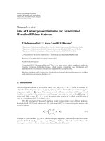
2.1. Measurement Setup. The measurement setup for the
MIMO measurements is shown in Figure 1 and is detailed
in the following along with the measurement procedure. A
network analyzer (Agilent E8257D) is used to measure the
complex channel frequency response for a set of transmitting
and receiving antenna positions. The channel is probed
in a 40 MHz measurement bandwidth from 3460 MHz to
3500 MHz. As transmitting (Tx) and receiving antenna
(Rx), broadband omnidirectional discone antennas of type
Electro-Metrics EM-6116 are used. These antennas can
operate in a range from 2 to 10 GHz with a nominal gain
of 1 dBi. The gain variation in the measured frequency range
is less than 0.5 dB, which shows a sufficiently flat antenna
frequency response. The vertical half-power beamwidth of
the antenna is 60
◦
. To be able to perform measurements for
large Tx-Rx separations, one port of the network analyzer
is connected to the Tx through an RF/optical link with an
optical fiber of length 500 m. The RF signal sent into the Tx
is amplified using an amplifier of type Nextec-RF NB00383
with an average gain of 37 dB. The amplifier assures that
the signal-to-noise ratio at the receiving port of the network
analyser is at least 20 dB for each measured location of the
Tx and Rx. The calibration of the network analyzer is done at
the connectors of the Tx and Rx antenna and as such includes
both the RF/optical link and the amplifier.

Measurements are performed using a v irtual MIMO
array [10]. The virtual array is created by moving the
antennas to predefined positions along rails in two directions
in the horizontal plane. The polarization of both Tx and
Rx is vertical for all measurements. For this, stepper motors
with a spatial resolution of 0.5 mm are used. Both Tx and Rx
are moved along 10 by 4 virtual uniform rectangular arrays
(URAs) and are positioned at a height of 1.80 m during
measurements (Figure 1). Both antennas were used at the
same height of 1.80m because of practical considerations
with the usage of the measurement system, most importantly
to keep the antennas far enough away from the rails
of the positioning system as possible while also avoiding
vibrations of the antennas. The URA elements are spaced
4.29 cm apart, which corresponds to half a wavelength at the
highest measurement frequency of 3.5 GHz and ascertains
that spatial aliasing does not occur when estimating the
directional characteristics of propagation paths [11]. The
stepper motor controllers, as well as the network analyzer,
are controlled by a personal computer (PC).
One important drawback of using a virtual array is that
the surroundings have to remain stationary during the mea-
surement. To assure this, measurements are done at night
in the absence of (people) movement. Furthermore, one
measurement location was done per night with fluorescent
lights switched on only in the hallway. We therefore only
expect a few paths impinging on switched-on lights which
would not be stationary [12]. At each of 1600 (10
×4×10×4)
combinations of Tx and Rx positioning along the URAs, the

network analyser measured the S
21
scattering parameter ten
times (i.e., 10 time observations). The total measurement
time for a single MIMO measurement is about 1 h 30 min.
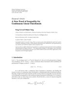
2.2. Measurement Environment. MIMO measurements are
carried out on the first floor of an office building. The office
floor has a rectangular shape with dimensions 57.9 m by
14.2 m. Figure 2 presents a floor plan of the measurement
environment, along with some relevant dimensions. The
office floor consists of a hallway, which stretches horizontally
in the center of Figure 2 and leads to various offices at the
top and bottom in the figure. All inner walls are plasterboard,
except for the concrete walls between rooms 118 and 120, and
between rooms 115 and 117. Figure 2 also shows locations
of the Tx and Rx during measurements. A total of 9 MIMO
measurements are performed; their Tx and Rx locations
EURASIP Journal on Wireless Communications and Networking 3
RF to optical
RF
RF
RF
RF
Optical fiber
Optical to RF
Amplifier
PC
Network analyzer
Tx
Rx

1.8 m
1.8 m
4.29 cm 4.29 cm
4.29 cm
4.29 cm
10by4TxURA 10by4RxURA
Figure 1: Measurement setup.
are indicated by couples of Tx
i
and Rx
i
(i = 1, ,9).
Measurements are executed in both line-of-sight (LoS) and
non-line-of-sight (nLoS) conditions and co ver distances
between Tx and Rx from 13 to 45 m. Measurement locations
1, 5, and 6 are LoS. Measurements were performed with
the doors of the offices closed. The measurement points
were selected to make the propagation conditions as diverse
as possible in this environment; they include hallway-to-
hallway, hallway-to-room, and room-to-room propagation.
Additionally, the Tx-Rx line sometimes intersects with only
plasterboard walls and sometimes with both plasterboard
and concrete walls.
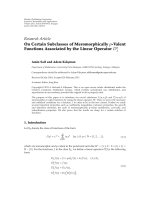
Figure 3(a) shows a picture of the hallway together with
the receiving virtual array. The hallway is free of any furniture
or clutter otherwise. Figure 3(b) shows a typical office on this
floor together with the transmitting virtual array. The offices
contain clutter comprising (wood and metal) desks, chairs,
desktop PCs, and (metal) filing cabinets.
2.3. Parameter Extraction and Clustering

2.3.1. Extraction of Directional and Delay Properties of
Propagation Paths. The directional azimuth of arrival (AoA)
and azimuth of departure (AoD) parameters and the delay
parameter of propagation paths or multipath components
(MPCs) are extracted from measurement data using a 5D
unitary ESPRIT (estimation of signal parameters via rota-
tional invariance techniques) algorithm [13]. The ESPRIT
algorithmisreferredtoas5D,becauseelevationsofarrival
and departure are also incorporated in its data model; this
alleviates the issue of biased azimuthal angle estimates when
only the azimuthal cut is present in the data model [14, 15].
Statistics of the elevation angles are however left out from
further analysis in this paper, as these angles possess the
“above-below” ambiguity inherent to URAs. The ESPRIT
algorithm is used in combination with the simultaneous
Schur decomposition procedure for automatic pairing of
AoA, AoD, and delay estimates [16]. The coordinate system
with respect to which AoA and AoD are defined is shown in
Figure 2.
URAs allow easy application of the spatial smoothing
technique to increase the number of observations while at
thesametimeincreasethedetectionpossibilitiesofcoherent
or correlated MPCs [17]. A downside to the technique is
the reduced estimation accuracy when the dimensions of the
URA subarrays are chosen too small. A possible compromise
chooses sub-URAs with dimensions 2/3ofthelengthin
each direction of the original 10 by 4 URA (rounded to
the nearest integer), that is, 7 by 3 su b-URAs [18]. In
total at both link ends, 64 different 7 by 3 sub-URAs can
be found, thereby increasing t he number of observations

by a factor of 64. Together with the previously mentioned
10 time observations (Section 2.1), the total number of
available observations is 640. Furthermore, in the 40 MHz
measurement bandwidth, 10 equally spaced frequency points
are used with the ESPRIT algorithm. Summarizing, 5D
unitary ESPRIT is applied to a 5D vector space of size 7
×
3 × 7 × 3 × 10 (spatial dimensions of size 7 and 3 following
from each the Tx and Rx URA, and the frequency dimension
of size 10) w ith 640 obser vations.
4 EURASIP Journal on Wireless Communications and Networking
Rx
1
Rx
2
Rx
3
Rx
4
Rx
5
Rx
7
Rx
8
Rx
9
Tx
1
Tx

2
Tx
3
Tx
4
Tx
5
Tx
6
Tx
7
Tx
8
Tx
9
8.1 m
1.9 m
4.2 m
14.2 m
57.9 m
AoA
or AoD
X
Y
106
108
110
112
114
116

118
120
122
103
105
107
109
111
113
115
117
119
121
123
125
Rx
6
Figure 2: Floor plan of the measurement environment with Tx and Rx locations.
(a) Hallway + Rx (b) Office + Tx
Figure 3: Photos of the measurement environment including the virtual arrays.
The ESPRIT algorithm is used to estimate the 100 most
strongest paths from measurement data [9, 19]. Next, the
estimated MPCs are postprocessed in the delay domain by
considering the power delay profile (PDP, i.e., MPC power
versus delay). For a typical PDP, power is concentrated at
small delays while at large delays only the noise floor remains.
In our measurements, the noise floor is set to the power of
the MPC with the largest delay. Following, all MPCs with
power less than the noise floor plus a noise threshold of 6 dB
are omitted from further analysis [9]. For all measurement

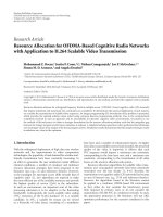
locations after postprocessing, between 35 and 87 MPCs are
retained. Figure 4(a) shows an AoA/AoD/delay scatter plot of
MPCs detected at measurement location 1. The power on a
dB scale of each MPC is indicated by a color.
2.3.2. Clu stering of Pr opagation Paths. For our data, auto-
matic joint clustering of AoA, AoD, and delay is performed
using the statistical K-power-means algorithm [20]. The
K-power-means algorithm result is in agreement with the
COST 273 definition of a cluster as a set of MPCs with similar
propagation characteristics [8]. Because some parameters
for clustering are circular, multipath component distance
(MCD) is used as the distance measure for clustering [ 21].
A delay scaling factor of 5 was used with the MCD , the same
value as used for clustering in indoor office environments in
[9].
For each measurement location, the number of clusters
for the K-power-means algorithm is varied between 2 and
10. The optimal number of clusters is selected according to
the Kim-Parks index [22]. The Kim-Parks index is preferred
over other more common validity indices that make use of
intracluster and intercluster separation measures, such as
the Davies-Bouldin and Cali
˜
nski-Harabasz indices, as these
indices tend to decrease or inc rease monotonically with the
number of clusters [23]. The Kim-Parks index circumvents
this behavior by normalizing the index by the index values at
the minimum and maximum number of clusters. The Kim-
Parks index is, for example, also used for MPC clustering
in [19]. The number of detected clusters varies from 3

to 8 between measurement locations, and for all MIMO
measurements combined, a total of 4 5 clusters are found (16
clusters from LoS and 29 clusters from nLoS measurements).
Next, to ease the statistical analysis, clearly outlying MPCs are
removed from each cluster using the shapeprune algorithm
detailed in [20]. To preserve the cluster’s original power and
shape, outliers are discarded with the restraint that the total
EURASIP Journal on Wireless Communications and Networking 5
cluster power and the cluster rms AoA, AoD, and delay
spreads remain within 10% of their values prior to outlier
removal.
After pruning outliers, the average cluster rms AoA
and AoD spreads amount to 22
◦
and 36
◦
, respectively. For
comparison, cluster rms azimuthal spreads between 2
◦
and
9
◦
were found in [24]. The main reason for the larger
spread values obtained here is that the clustering for our
measurements takes the delay domain into account, while the
study in [24] restricts clustering to the AoA/AoD domains.
It is also mentioned in their work that restricting clustering
to the azimuthal domains results in more clusters and hence
smaller spread values. The spread values obtained here
comparemoretothoseintherelatedworkof[24], where

values between 22
◦
and 27
◦
are found. Next, cluster rms
delay spreads vary between 0.5 and 3.4 ns for LoS. For nLoS,
cluster rms delay spreads are between 0.4 and 9.9 ns and are
comparable to spreads between 2 and 15 ns found in [19].
Furthermore, the physical realism of clusters was verified
by visually cross-referencing cluster mean angles and mean
delay (mean propagation distance) with the floor plan in
Figure 2. This verification procedure is similar to the one
applied in [25], although in this work the procedure is
automated with a ray tracer.
Figure 4(b) shows a scatter plot of the clustering result
for measurement location 1. For this measurement, the Kim-
Parks index estimated the number of clusters at 7. MPCs
grouped into different clusters are shown with different
marker shapes and colors.
2.4. Limitations of the Measurement Methodology. This sec-
tion lists the limitations of the MPC measurement methodol-
ogy. These arise from restrictions of the measurement system
in Section 2.1 and could be possible sources of errors in the
discussion of the clustered MPC results in Sections 4 and 5.
(i) A full polarimetric antenna radiation pattern is
not available for calibration. As such, MPC results
presented here include nonchannel antenna effects.
(ii) MPC results are only available for vertical (Tx) to
vertical (Rx) polarization. Horizontal polarization
is thus missing. Additionally, because a full polari-

metric antenna model is lacking, it is not known
if the measurement antennas’ cross-polarization dis-
crimination is large enough to sufficiently limit
power leakage from the horizontal to the vertical
polarization.
(iii) Unambiguous results for the MPC elevation parame-
ter are not available due to the use of planar antenna
arrays. The missing elevation parameter will affect
clustering results; inclusion of an extra parameter will
often result in smaller clusters b ecause of the extra
dimension in which MPCs can be discriminated.
3. Model
3.1. Signal Model. For the analysis of the intracluster and
intercluster propagation path parameters, we use the fol-
lowing basic signal model, based on the double-directional
channel model first proposed in [26]. Contrary to the
double-directional model, the basic signal model described
here includes the Tx and Rx antenna radiation patterns as
part of the channel.
For one of the measurement locations, t he complex
received envelope h(φ
A
, φ
D
, τ) is written as function of the
propagation path parameters: φ
A
denotes the AoA, φ
D
is the

AoD, a nd τ isthepathdelay.TheuseofMPCclustersis
reflected in the complex envelope’s notation
h

φ
A
, φ
D
, τ

=
n
C

c=1
n
P,c

k=1
A
c,k
· δ

φ
A
− Φ
A
c,k

×

δ

φ
D
− Φ
D
c,k

δ

τ − T
c,k

.
(1)
In (1), n
C
is the number of clusters and n
P,c
is the number
of MPCs within cluster c.Forthekth propagation path in
cluster c, A
c,k
is its received complex amplitude, Φ
A
c,k
and
Φ
D
c,k

are its AoA and AoD , respectively, and T
c,k
is its delay.
δ(
·) denotes the Dirac delta function. We also define P
c,k
as
the power of path k in cluster c,thatis,P
c,k
= E[|A
c,k
|
2
]
where the expectation operator E[
·] is taken over all 640
time observations. Instead of directly modelling the statistics
of the complex amplitude A
c,k
, the path’s power P
c,k
will
be modelled. To allow statistical analysis of propagation
parameters of all measurement locations collectively, the
dependence of power P
c,k
and delay T
c,k
on distance is
removed. Power is rescaled such that the total received MPC

powerequalsone,andtheoriginofthedelayaxisissetto
coincide with the first arriving MPC. Assuming larger values
of c or k mean later arriving paths
n
C

c=1
n
P,c

k=1
P
c,k
= 1, T
1,1
= 0ns.
(2)
We propose to extend the signal model in (1)by
splitting up each of the propagation path parameters into an
intercluster and an intracluster part
A
c,k
=

p
c
a
c,k
,
P

c,k
= p
c
p
c,k
,
Φ
A
c,k
= φ
A
c
+ φ
A
c,k
,
Φ
D
c,k
= φ
D
c
+ φ
D
c,k
,
T
c,k
= τ
c

+ τ
c,k
.
(3)
In (3), the parameters p
c
, φ
A
c
, φ
D
c
,andτ
c
denote
intercluster propagation parameters and are representative
for the location of each cluster in the power/AoA/AoD/delay
parameter space. Also in (3), a
c,k
, p
c,k
, φ
A
c,k
, φ
D
c,k
,andτ
c,k
are intracluster propagation parameters. The intracluster

parameters can be seen as the deviations of individual paths
from the cluster’s location as dictated by the intercluster
parameters. The intracluster parameters are therefore fully
determined by the spr ead of power, AoA, AoD, and delay in
6 EURASIP Journal on Wireless Communications and Networking
0
90
180
270
360
0
90
180
270
360
160
170
180
190
Delay (ns)
Power (dB)
−90
−85
−80
−75
−70
−65
−60
−55
−50

−45
−40
Ao
D(
◦
)
AoA (
◦
)
(a) MPC AoA/AoD/delay scatter plot
0
90
180
270
360
0
90
180
270
360
160
170
180
190
Delay (ns)
AoD (
◦
)
AoA(
◦

)
(b) MPC K-power-means clustering
Figure 4: MPC scatter plot and clustering for measurement location 1 (LoS).
each of the clusters. With the definitions in (3), the signal
model in (1) is rewritten as
h

φ
A
, φ
D
, τ

=
n
C

c=1
n
P,c

k=1

p
c
a
c,k
· δ

φ

A
− φ
A
c
− φ
A
c,k

×
δ

φ
D
− φ
D
c
− φ
D
c,k

δ

τ − τ
c
− τ
c,k

.
(4)
Section 4 discusses the statistical distributions of P

c,k
, Φ
A
c,k
,
Φ
D
c,k
,andT
c,k
within each cluster. The most common prob-
ability distributions are location-scale distributions; they are
parameterized by a location parameter, which determines the
distribution’s location or shift, and a scale parameter, which
determines the distribution’s dispersion or spread. These
two types of distributional parameters can fully describe
the intercluster and intracluster propagation parameters, and
hence the signal model in (4); the distributional location
parameter can be identified with the intercluster propagation
parameter, and the distributional scale parameter fully
characterizes the intracluster propagation parameter. The
distributional location and scale parameters are further
discussed in Section 5.
3.2. FABLE Notation. The goal of this section is to provide a
new notation for the MIMO channel matrix. This notation
is named FActorization into a BLock-diagonal Expression or
FABLE [27, 28]. The appeal of the FABLE notation laid
outhereisinitsfutureincorporationinthedatamodel
of multipath estimation algorithms. The FABLE notation
further subdivides each of the angular and delay dimensions

into an intra- and intercluster subdimension. This subdivi-
sion has the potential to further reduce the computational
complexity of space-alternating estimation algorithms, as
the harmonic retrieval problem is broken down into more
dimensions. For appropriate antenna arrays at transmit and
receiveside,thetransformationof(4) to aperture space is
given by
H

r, s, f

=
n
C

c=1
n
P,c

k=1

p
c
a
c,k
· e
− j2π(r−1)G
Rx
(φ
A

c
+φ
A
c,k
)
× e
− j2π(s−1)G
Tx
(φ
D
c
+φ
D
c,k
)
e
− j2πf(τ
c
+τ
c,k
)
.
(5)
In (5), the variables r, s,and f denote the transform variables
of the Fourier transform of φ
A
, φ
D
,andτ, respectively. Each
(integer) value of r and s can be associated with one of

the antennas of the Rx and Tx antenna array. The variable
f denotes the frequency o f the transmitted signal. The
functions G
Rx
(·)andG
Tx
(·) depend on the Rx and Tx array
geometry. For example, G
Rx
(·) = G
Tx
(·) = (d/λ)sin(·)for
uniform linear arrays (ULAs) at receive and transmit side,
where d is the spacing between antenna array elements, and
λ is the wavelength.
In the following, it is assumed that the array geometry
functions G
Rx
(·)andG
Tx
(·) are linear, that is, that in (5)it
holds that G
Rx
(φ
A
c
+ φ
A
c,k
) = G

Rx
(φ
A
c
)+G
Rx
(φ
A
c,k
) and analo-
gously G
Tx
(φ
D
c
+ φ
D
c,k
) = G
Tx
(φ
D
c
)+G
Tx
(φ
D
c,k
). Unfortunately,
this assumption is usually not valid, for example, for the

ULA, URA, and uniform circular array (UCA) geometries.
This can be remedied by transforming the intercluster and
intracluster angular propagation parameters. For example,
for the receive side, the FABLE notation in the following
can be used with ψ
A
c
and ψ
A
c,k
as intercluster and intracluster
AoA, respectively, for which it is satisfied that G
Rx
(Φ
A
c,k
) =
G
Rx
(ψ
A
c
)+G
Rx
(ψ
A
c,k
). For example, for a ULA, this can
be shown to hold if ψ
A

c
and ψ
A
c,k
are defined such that
sin(ψ
A
c
) = sin(φ
A
c
)cos(φ
A
c,k
)andsin(ψ
A
c,k
) = cos(φ
A
c
)sin(φ
A
c,k
).
This transformation can be done without consequence as
there an inherent arbitrariness on how the AoA is split
up into its respective inter- and intracluster parts. The
disadvantage of redefining the inter- and intracluster AoA is
that Φ
A

c,k
/
= ψ
A
c
+ψ
A
c,k
, contrary to the definition with φ-s in (3).
EURASIP Journal on Wireless Communications and Networking 7
This means that, unlike the definition with φ-s, the inter- and
intracluster AoAs defined as ψ-s cannot be quickly related to
the corresponding MPC AoA Φ
A
c,k
and also depend on the
array geometry function G
Rx
(·) under consideration.
We assume that the Rx and Tx antenna arrays consist of
R and S antenna elements, respectively (r
= 1, , R and s =
1, , S). The MIMO channel transfer function H (r, s, f )
is first rewritten as the MIMO channel matrix H( f ). The
channel matrix H has the common structure where the row
dimension of H is made up from receive elements r and
its column dimension is made up from transmit elements
s (H has dimensions R
× S). The channel matrix H( f )is
decomposed as the product of three matrices

H

f

=
B
Rx

f

·
W

f

·
B
Tx
.
(6)
In (6), B
Rx
( f )andB
Tx
contain intercluster propagation
parameters associated with the Rx and Tx, respectively.
By choice, the intercluster parameters p
c
, φ
A

c
,andτ
c
are
considered to be properties of cluster c as seen by the R x,
while φ
D
c
is considered to characterize cluster c as seen
from the Tx. Because of the choice to house delay τ
c
in
B
Rx
( f ), the elements of this matrix depend on the frequency
f .Alsoin(6), W( f ) gathers the intracluster propagation
parameters a
c,k
, φ
A
c,k
, φ
D
c,k
,andτ
c,k
.ThematricesB
Rx
, W,and
B

Tx
are built from submatrices B
Rx
c
, W
c
,andB
Tx
c
, respectively,
which contain the intercluster and intracluster propagation
parameters solely associated with cluster c.Thestackingof
these submatrices is conceived as follows (the f dependency
is left out for better readability):
H
= B
Rx
· W · B
Tx
=

B
Rx
1
B
Rx
2
··· B
Rx
n

C

·
⎡
⎢
⎢
⎢
⎢
⎢
⎢
⎢
⎣
W
1
0 ··· 0
0W
2
··· 0
.
.
.
.
.
.
.
.
.
.
.
.

00
··· W
n
C
⎤
⎥
⎥
⎥
⎥
⎥
⎥
⎥
⎦
·
⎡
⎢
⎢
⎢
⎢
⎢
⎢
⎢
⎣
B
Tx
1
B
Tx
2
.

.
.
B
Tx
n
C
⎤
⎥
⎥
⎥
⎥
⎥
⎥
⎥
⎦
.
(7)
The stacking of the submatrices W
c
gives rise to a block-
diagonal form for the intracluster matrix W,fromwhichthe
name FABLE is derived.
3.2.1. Intercluster Submatrices B
Rx
c
and B
Tx
c
. For cluster c,
the submatrices B

Rx
c
and B
Tx
c
have the following structure
(diag(
·) represents a diagonal matrix with its arguments
along the main diagonal):
B
Rx
c
=

p
c
e
− j2πfτ
c
· diag

1, e
− j2πG
Rx
(φ
A
c
)
, , e
− j2π(R−1)G

Rx
(φ
A
c
)

,
B
Tx
c
= diag

1, e
− j2πG
Tx
(φ
D
c
)
, , e
− j2π(S−1)G
Tx
(φ
D
c
)

.
(8)
It is clear that B

Rx
c
only contains intercluster propagation
parameters associated with the Rx: the cluster mean AoA
φ
A
c
,theclusteronsetτ
c
at receive side, and the cluster
median received power p
c
.ThesubmatrixB
Tx
c
contains the
intercluster parameter associated with the Tx, that is, the
cluster mean AoD φ
D
c
.ThesubmatricesB
Rx
c
and B
Tx
c
have
dimensions R
× R and S × S, respectively.
3.2.2. Intracluster Submatrix W

c
. For cluster c,thesubmatrix
W
c
is written as the product of three matrices
W
c
= V
Rx
c
· D
Rx
c
· V
Tx
c
.
(9)
The three matrices V
Rx
c
, D
Rx
c
and V
Tx
c
possess the following
structure
V

Rx
c
=
⎡
⎢
⎢
⎢
⎢
⎢
⎢
⎢
⎢
⎣
11··· 1
e
− j2πG
Rx
(φ
A
c,1
)
e
− j2πG
Rx
(φ
A
c,2
)
··· e
− j2πG

Rx
(φ
A
c,n
P,c
)
.
.
.
.
.
.
.
.
.
.
.
.
e
− j2π(R−1)G
Rx
(φ
A
c,1
)
e
− j2π(R−1)G
Rx
(φ
A

c,2
)
··· e
− j2π(R−1)G
Rx
(φ
A
c,n
P,c
)
⎤
⎥
⎥
⎥
⎥
⎥
⎥
⎥
⎥
⎦
,
D
Rx
c
= diag

a
c,1
e
− j2πf(τ

c,1
)
, a
c,2
e
− j2πf(τ
c,2
)
, , a
c,n
P,c
e
− j2πf(τ
c,n
P,c
)

,
V
Tx
c
=
⎡
⎢
⎢
⎢
⎢
⎢
⎢
⎢

⎢
⎣
1 e
− j2πG
Tx
(φ
D
c,1
)
··· e
− j2π(S−1)G
Tx
(φ
D
c,1
)
1 e
− j2πG
Tx
(φ
D
c,2
)
··· e
− j2π(S−1)G
Tx
(φ
D
c,2
)

.
.
.
.
.
.
.
.
.
.
.
.
1 e
− j2πG
Tx
(φ
D
c,n
P,c
)
··· e
− j2π(S−1)G
Tx
(φ
D
c,n
P,c
)
⎤
⎥

⎥
⎥
⎥
⎥
⎥
⎥
⎥
⎦
.
(10)
V
Rx
c
and V
Tx
c
are Vandermonde matrices which contain
for cluster c the intracluster AoAs φ
A
c,k
and the intracluster
AoDs φ
D
c,k
, respectively, (k = 1, , n
P,c
). The d iagonal matrix
D
Rx
c

comprises the received intracluster complex amplitude
a
c,k
and the intracluster delay τ
c,k
(k = 1, , n
P,c
). The
matrices V
Rx
c
, D
Rx
c
,andV
Tx
c
have dimensions R × n
P,c
, n
P,c
×
n
P,c
,andn
P,c
× S, respectively.
As a closing remark, the FABLE notation in (7)can
intuitively be understood as follows. Firstly, clusters with
their average directional characteristics are created at trans-

mit side by the matrix B
Tx
. Next, the block-diagonal W
matrix introduces several discrete paths into each cluster. The
matrix W can be thought of as the operator which unfolds
each cluster into its discrete paths. Finally, the matrix B
Rx
c
describes how the clusters’ average directional characteristics
are seen by the Rx when they arrive at receive side.
4. Stat istics of the MPC Parameters
This section discusses the statistical distributions within each
cluster of the MPC parameters Φ
A
c,k
, Φ
D
c,k
, T
c,k
,andP
c,k
.
Preliminarily, the correlations between these four parameters
are investigated to check whether they can be modelled
separately by univariate distributions. A summary of this
section’s results is found in Tabl e 2, near the end of the paper.
4.1. Correlations. In this section, correlations between
azimuthal angles Φ
A

c,k
and Φ
D
c,k
,delayT
c,k
,andpowerP
c,k
are calculated. The measure of correlation used is Spearman’s
8 EURASIP Journal on Wireless Communications and Networking
Table 1: Average Spearman’s correlation of MPC parameters within
each cluster and success rates for zero correlation.
Average Spearman’s
correlation [
−]
Success rates at 5%/1% significance [%]
Φ
D
c,k
T
c,k
P
c,k
Φ
D
c,k
T
c,k
P
c,k

Φ
A
c,k
0.04 −0.12 0.18 100.0/100.0 88.9/95.6 86.7/95.6
Φ
D
c,k
−0.01 −0.09 95.6/100.0 95.6/100.0
T
c,k
−0.28 80.0/93.3
rank correlation coefficient [29]. This correlation coefficient
is nonparametric in the sense that it does not make any
assumptions on the form of the relationship between the
two variables, other than being a monotonic relationship.
Spearman’s correlation is calculated between the four MPC
parameters on a per-cluster basis. For the MPCs in cluster
c, Spearman’s correlation coefficient ρ
c
(X
c,k
, Y
c,k
) between
MPC parameters X
c,k
and Y
c,k
is given by (X
c,k

, Y
c,k
= Φ
A
c,k
,
Φ
D
c,k
, T
c,k
,orP
c,k
)
ρ
c

X
c,k
, Y
c,k

=
1 −
6

n
P,c
k=1


x
c,k
− y
c,k

2
n
P,c


n
P,c

2
− 1

.
(11)
In (11), x
c,k
and y
c,k
represent the statistical ranks of X
c,k
and Y
c,k
. Before calculating their ranks, the azimuthal angle
variables are restricted to their principal value in (
−π, π]to
avoid the 2π ambiguity.

Table 1 shows average values of ρ
c
(X
c,k
, Y
c,k
) taken over
all 45 clusters detected in the measurement campaign.
Table 1 shows fairly weak average correlations between
the MPC parameters. The strongest correlation is found
between path power P
c,k
and path delay T
c,k
(negative
average correlation of
−0.28). This correlation is expected
and well established by the S aleh-Valenzuela model, where
power decay within a cluster is modeled as a monotoni-
cally decreasing exponential function of delay [30]. For all
ρ
c
(X
c,k
, Y
c,k
), hypothesis tests (nonparametric permutation
tests) are carried out to decide whether or not the correlation
coefficients differ significantly from zero. Ta ble 1 lists the
success rates of these tests, that is, for which percentage

of clusters the test decided in favor of zero correlation,
at both the 5% and 1% significance level. Ta ble 1 shows
that, for most clusters, the MPC parameter correlations can
be assumed to be zero (success rates of more than 80%
and more than 93% at the 5% and 1% significance level,
resp.). As expected, the success rates are the lo w est for
correlation between P
c,k
and T
c,k
,forwhichthestrongest
correlation was found. Concluding, correlations between
MPC parameters within clusters can be assumed to be weak
and often indistinguishable from zero. Therefore, the MPC
parameters Φ
A
c,k
, Φ
D
c,k
, T
c,k
,andP
c,k
are modelled separately
by univariate distributions in the next sections, without
taking any relationships between them into account.
Alternatively, correlation coefficients can also be calcu-
lated with the parametric circular-linear and circular-circular
correlation coefficients defined in [31]. These correlation

coefficients are designed to work with circular data (in
our case, the azimuthal angles). Using these correlation
coefficients, average correlation values are somewhat larger
than those for Spearman’s correlation in Table 1 and range
from
−0.27 to 0.49. Hypothesis tests for zero correlation at
the 5% significance level however still deliver success rates
of more than 84%, supporting the previous decision of
modelling the MPC parameters univariately.
4.2. Azimuths of Arrival Φ
A
c,k
and Departure Φ
D
c,k
. In this
section, we discuss the marginal distributions of AoAs Φ
A
c,k
and AoDs Φ
D
c,k
for each individual cluster c. In literature,
various distributions are proposed for the azimuth angles
within a certain cluster. In [9], a normal distribution is
chosen where realisations are mapped to their principal value
in (
−π, π]. A Laplacian distribution for the azimuth angles
is first proposed in [32]. Additionally, we consider the von
Mises distribution [33]. The von Mises distribution can be

thoughtofasananalogueofthenormaldistributionfor
circular data. Special consideration is given to this distri-
bution, because in our opinion, the von Mises distribution
seems natural in describing the statistics of azimuth data;
the support of the von Mises distribution is an interval of
length 2π, the same as the support of azimuth data, while
the support of the normal and Laplacian distribution is an
interval of infinite length. For example, for the AoAs Φ
A
c,k
in
cluster c, the von Mises probability density function (pdf)
p
vM
(Φ
A
c,k
; α
A
c
, κ
A
c
)isgivenas
p
vM

Φ
A
c,k

; α
A
c
, κ
A
c

=
exp

κ
A
c
cos

Φ
A
c,k
− α
A
c

2πI
0

κ
A
c

,

k
= 1, , n
P,c
.
(12)
In (12), I
0
(·) is the modified Bessel function of the zeroth
order. The two parameters that characterize the von Mises
pdf are α
A
c
, the circular mean of Φ
A
c,k
,andκ
A
c
,whichisa
measure of concentration of Φ
A
c,k
angles around α
A
c
.
The most fit distributions for the intracluster AoAs and
AoDs are investigated as follows. From the azimuth angles
Φ
A

c,k
and Φ
D
c,k
, the maximum likelihood estimators (MLEs)
of the parameters of the normal, Laplacian, and von Mises
pdf are calculated separately for the AoAs and AoDs of
each cluster c.Forclusterc, the likelihood of observing the
samples Φ
A
c,k
(analogously Φ
D
c,k
)fork = 1, , n
P,c
as possible
outcomes under each of the three statistical distributions
(with the MLEs as distributional parameters) is calculated.
The most fit distribution is determined by performing simple
likelihood ratio tests (LRTs); the statistical distribution
which renders the largest likelihood is most appropriate
for describing the azimuth angle statistics for that cluster.
For the 45 clusters in this measurement campaign, all LRTs
decided in favor of the von Mises distribution for both
Φ
A
c,k
and Φ
D

c,k
. Figure 5 shows the empirical cumulative
distribution function (CDF) of the AoAs Φ
A
c,k
of a cluster
at measurement location 5. Also shown are the estimated
CDFs of the Von Mises, normal, and Laplacian distribution.
Visually, it could be concluded from Figure 5 that all three
investigated theoretical distributions provide a reasonable fit
to the empirical data, and that any of these distributions
EURASIP Journal on Wireless Communications and Networking 9
−90 −45 0 45 90 135 180 225 270
0
0.1
0.2
0.3
0.4
0.5
0.6
0.7
0.8
0.9
1
Φ
A
c,k
(
◦
)

Prob (Φ
A
c,k
< abscissa)
Empirical CDF
Von Mises CDF
Normal CDF
Laplace CDF
Figure 5: CDF plot o f Φ
A
c,k
and estimated theoretical CDFs for a
cluster at measurement location 5.
could be chosen for modelling the AoA. However, the LRTs
allow to quantitatively measure the goodness of fit and decide
in favor of the von Mises distribution.
4.3. Delay T
c,k
. In this section, the statistics within each
cluster c of the delay parameter T
c,k
are discussed. The
marginal distribution of the delay parameter can be modeled
in a number of ways. In [9], MPC delays within a cluster are
assumed to be normally distributed. A possible issue with
this modeling approach is that MPC delays inherently only
take on positive values, which does not match the support
of the normal distribution. To avoid this issue, MPC delays
T
c,k

within cluster c are modelled according t he principle laid
out by the well-known, cluster-based Saleh-Valuenzuela (SV)
model [30]. Herein, the waiting time between the arrival of
two consecutive MPCs within a certain cluster is modelled
by an exponential distribution. For the MPCs in cluster c
(assuming the delays are ordered such that T
c,1
<T
c,2
<
··· <T
c,n
P,c
), the exponential pdf p
exp
(T
c,k
| T
c,k−1
; λ
c
)as
function of the delay T
c,k
of the kth MPC , given that the
(k
− 1)th MPC arrived at known delay T
c,k−1
,iswrittenas
p

exp

T
c,k
| T
c,k−1
; λ
c

=
1
λ
c
exp

−
T
c,k
− T
c,k−1
λ
c

,
k
= 2, , n
P,c
.
(13)
In (13), the exponential distribution has the parameter

λ
c
which corresponds to the mean waiting time between
consecutive MPCs in cluster c. An additional distributional
parameter θ
c
is defined as the delay of the first arriving path
in cluster c,thatis,θ
c
= T
c,1
,asT
c,1
does not follow from
(13).
For each cluster c, the mean waiting time λ
c
is estimated
by its MLE following from the exponential distribution. The
plausibility of an exponential distribution for the arrival
0 0.5 1 1.5 2
Theoretical quantiles (exponential, λ
c
= 0.53 ns)
0
0.5
1
1.5
2
Empirical quantiles (T

c,k
− T
c,k−1
)
Figure 6: QQ plot of quantiles of T
c,k
− T
c,k−1
versus quantiles of an
exponential distribution for a cluster at measurement location 3.
times T
c,k
is then validated by executing an Anderson-
Darling (AD) goodness-of-fit test for composite exponential-
ity [34]. For the 45 clusters in the measurement campaign,
the minimum, average, and maximum P values associated
with the AD test are equal to .06, .40, and .92, respectively.
This means that, at the 5% significance level, all 45 clusters
retain exponentiality. Figure 6 shows the quantile-quantile
(QQ) plot of the empirical quantiles of samples T
c,k
−
T
c,k−1
versus the theoretical quantiles of the exponential
distribution (13) for a cluster detected at measurement
location 3 (the MLE of λ
c
equals 0.53 ns). Figure 6 sho ws
good agreement of the waiting times in this cluster with an

exponential distribution.
4.4. Power P
c,k
. A natural model for the fading of MPC
powers P
c,k
in cluster c is the lognormal fading model [35,
36]. For cluster c, it is investigated whether the samples P
c,k
on a dB scale could originate from a normal distribution.
This normal distribution is parameterized by the mean
μ
c
and the standard deviation σ
c
of P
c,k
in dB. These
distributional parameters are estimated by their MLEs.
Composite normality of P
c,k
[dB] is assessed with a few
statistical tests in literature such as the Anderson-Darling
(AD) test [34], the Shapiro-Wilk (SW) test [37], and the
Henze-Zirkler (HZ) test [38]. Multiple tests for normality are
executed as no uniformly most powerful test exists against all
possible alternative distributions. The AD, SW, and HZ tests
are generally considered to be relatively powerful against a
variety of alternatives. Of the 45 clusters in this measurement
campaign, normality of P

c,k
[dB] is retained at the 5%
significance level for 39, 38, and 40 clusters with the AD,
SW, and HZ tests, respectively. For the 45 clusters, average
P values are .38 (AD), .43 (SW), and .44 (HZ). Concluding,
10 EURASIP Journal on Wireless Communications and Networking
normality for P
c,k
[dB] is assumed in the following, as
the majority of clusters pass the different goodness-of-fit
tests.
5. Stat istics of the Distributional Parameters
This section models the intercluster and intracluster propa-
gation parameters laid out in the sig nal model of Section 3
in (1), (3), and (4). The intercluster and intracluster propa-
gation parameters are fully determined by t he distributional
parameters of the location-scale distributions of the previ-
ous section. In the following, the intercluster propagation
parameters are identified with the location parameters of the
distributions, that is, for cluster c,
φ
A
c
α
A
c
(
von Mises circular mean of AoAs
)
,

φ
D
c
α
D
c
(
von Mises circular mean of AoDs
)
,
τ
c
θ
c

onset of delays

,
p
c
μ
c

normal mean of powers in dB

.
(14)
The intracluster propagation parameters are characterized
by the scale parameters of the distributions, that is, for t he
MPCs in cluster c,

φ
A
c,k
−→ κ
A
c
(
von Mises concentration of AoAs
)
,
φ
D
c,k
−→ κ
D
c
(
von Mises concentration of AoDs
)
,
τ
c,k
−→ λ
c

exponential mean waiting time between delays

,
p
c,k

−→ σ
c

normal standard deviation of powers in dB

.
(15)
In the following, the statistics of the distributional
parameters are discussed. Preliminarily, correlations between
these parameters are investigated. In this section, distinction
is made between distributional parameters originating from
LoS and nLoS measurements, and it is assessed whether
the parameters’ statistics differ significantly between LoS
and nLoS. A summary of this section’s results is found in
Table 2.
5.1. Correlations. Spearman’s rank correlation coefficient is
calculated between the location and scale parameters, and
the two number parameters n
C
and n
P,c
.45samplesfor
each of these parameters are available (45 clusters in this
campaign). Figures 7(a) and 7(b) show the upper triangles of
the correlation matrices of estimated parameters stemming
from LoS and from nLoS measurements. Permutation tests
are carried out to decide on the significance of each of
the correlations. Correlation coefficients which prove to
significantly d iffer from zero at a 5% level are marked with
the text “5%.” Correlation coefficients which are different

from zero at the more strict 1% significance level are marked
with a “1%” label. For correlations without a label, the
permutation test accepted the hypothesis of zero correlation
at the 5% significance level.
Firstly, we look at the correlations between the distribu-
tional parameters in (14)and(15) (part of the correlation
matrices inside the dashed rectangles in Figures 7(a) and
7(b)). Most notably, the correlation between cluster mean
power p
c
and cluster onset τ
c
proves to be strong at the 1%
significance level, and this for both LoS (negative correlation
of
−0.80, P value of 1.8·10
−4
) and nLoS (negative correlation
of
−0.58, P value of 9 .7 · 10
−4
). This is well established
in the Saleh-Valenzuela model, where linear cluster power
is modelled as exponentially decaying with cluster delay
[30]. This strong correlation cannot be easily ignored, so
p
c
is modelled through regression with τ
c
in the following.

Additionally, in Figure 7, some correlations are significant
at the 5% level but not at the 1% level. These correlations
can sometimes be explained from the expected propagation
physics; for example, regarding the positive correlation of
0.37 between σ
c
and λ
c
innLoS,itisexpectedthatthe
variability of MPC power σ
c
will be larger if the MPCs are
characterized by a larger λ
c
, that is, have delays that are
further in between. For simplicit y of the provided models,
we choose to not perform regression between distributional
parameters for which the correlation is significant at the 5%
level but not at the 1% level, also because these correlations
are between different distributional parameters for LoS and
nLoS. Summarizing, the distributional parameters will be
modelled by their marginal statistical distributions in the
next sections, except for the mean cluster power p
c
which
strongly depends on the cluster onset τ
c
.
Secondly, we look at the correlations with the number
parameters n

C
and n
P,c
(part of the correlation matrices
outside the dashed rectangles in Figures 7(a) and 7(b)). In
this paper, no model is provided for the number of paths
per cluster n
P,c
; MPC parameter extraction in Section 2.3.1
estimated the 100 strongest MPCs without deciding on the
actual number of paths through heuristics. Nevertheless, the
significant correlations with n
P,c
in Figure 7 can give infor-
mation about the effect of the number of paths per cluster
on the estimation accuracy of other cluster parameters, in
particular scale (dispersion) parameters. For example, at the
1% level, the correlation between n
P,c
and λ
c
is significant
for both LoS (negative correlation of
−0.73) and nLoS
(negative correlation of
−0.61). As clusters contain paths
with similar delay characteristics, it can be expected that a
larger number of paths n
P,c
will yield closer spacing of these

paths on t he delay axis, that is, smaller estimated values
of λ
c
. In contrast to this, the estimation of the other scale
parameters κ
A
c
, κ
D
c
,andσ
c
does not seem to be greatly affected
by n
P,c
.InFigure 7(a),thenumberofclustersn
C
is not
strongly correlated with the distributional parameters for the
LoS measurements. In Figure 7(a), for nLoS, t he correlation
between n
C
and the location φ
A
c
of the clusters on the AoA
axis is significant at the 5% level (negative correlation of
−0.39). However, as there is no physical basis to assume
that the arr ival angle of a cluster should depend on the total
number of arriving clusters, this correlation will not be taken

into account while modelling the statistics of n
C
.
From the data in Figure 7,theconclusionisthata
majority of the correlations can be assumed to be zero, which
means that the multivariate postulation can be weakened
EURASIP Journal on Wireless Communications and Networking 11
φ
A
c
φ
D
c
τ
c
p
c
κ
A
c
κ
D
c
λ
c
σ
c
n
C
n

P,c
1
0.5
0
−0.5
−1
5%
5%
5%1%
1%
n
P,c
n
C
σ
c
λ
c
κ
D
c
κ
A
c
p
c
τ
c
φ
D

c
φ
A
c
(a) LoS measurements
5%
5%
5%
5%
1%
1%
1%
1%
φ
A
c
φ
D
c
τ
c
p
c
κ
A
c
κ
D
c
λ

c
σ
c
n
C
n
P,c
0
0
.5
−0.5
−1
n
P,c
n
C
σ
c
λ
c
κ
D
c
κ
A
c
p
c
τ
c

φ
D
c
φ
A
c
1
(b) nLoS measurements
Figure 7: Spearman’s correlation of distributional and number parameters
without completely moving to the univariate assumption.
Future work on this topic is to investigate whether or not
omitting correlations which are assumed to be zero would
significantly degrade channel matrix estimates. Finally, we
compare the correlation analysis in this section with the
observations made in [39]. In this work, strong correlations
between spreads in the AoA, AoD, and delay domains are
found, that is, clusters are small or large in all domains at
once. These strong correlations are not found for our mea-
surements ( see the correlations between the scale parameters
in Figure 7), except for LoS where κ
A
c
and κ
D
c
show significant
correlation. Contrary to [39], where an LoS/obstructed LoS
scenario is considered, our measurements also include a
heavy nLoS scenario with propagation through walls. For
our nLoS case, cluster spreads in all domains appear to be

decorrelated. For our LoS case, the azimuthal spreads are
significantly correlated as in [39]. However, in contrast to
this work, correlation with delay spread is weak for our
measurements, which is likely caused by our LoS cases being
restricted to hallway propagation.
5.2. Location Parameters (Intercluster)
5.2.1. Cluster Angular Means φ
A
c
and φ
D
c
. The uniform
distribution is a suitable distribution for modelling φ
A
c
and
φ
D
c
, as from a modelling perspective there is no physical
basis for a certain mean AoA or AoD to have a higher
probability of occurrence than another mean AoA or AoD.
In this section, no distinction is made between LoS and nLoS,
because the uniform distribution is not parameterized by any
distributional parameter (which could change between these
two circumstances). The premise of a uniform distribution in
(
−π, π] for the intercluster mean azimuth angles is validated
through statistical hypothesis tests. In [7], the popular

Kolmogorov-Smirnov (KS) test is advocated for goodness of
fit of the propagation para meters’ underlying distributions.
However, for small sample sizes, the KS test is known to
have low power. Because of this, we use Rao’s spacing test for
uniformity [40]. This test has the following advantages over
the KS test: it is designed for circular data, has higher power,
and is nonparametric which means that no error-prone
distributional assumption is made on the test statistic. For
both the 45 cluster mean AoAs φ
A
c
and the 45 cluster mean
AoDs φ
D
c
, Rao’s spacing test retained the null hypothesis of a
uniform distribution in (
−π, π]atthe5%significancelevel
(P values of .67 and .14, resp.).
5.2.2. Cluster Onset τ
c
. For consistency with the modelling of
the intracluster delay in Section 4.3,wealsoadopttheSaleh-
Valenzuela model for the intercluster delay; the waiting time
between the onsets τ
c
− τ
c−1
of two consecutively arriving
clusters is modelled by an exponential distribution [30].

This exponential distribution is fully parameterized by the
mean of waiting times τ
c
− τ
c−1
. Under the assumption of
an exponential distribution, it is first investigated whether
the mean waiting time between clusters differs between LoS
and nLoS measurements. This is done by executing the two-
sample Anderson-Darling (AD) test, which assesses whether
τ
c
− τ
c−1
grouped according to LoS or nLoS could both
originate from the same statistical distribution. This test
results in a P value of .04, which is borderline significant
at the 5% level and prompts us to distinguish between LoS
and nLoS. Next, for LoS and nLoS separately, composite
exponentiality of τ
c
−τ
c−1
is verified using the one-sample AD
test. An exponential distribution is accepted for both LoS and
nLoS at the 5% significance level (P values of .13 and .12,
resp.). The mean of waiting times τ
c
− τ
c−1

is estimated at
2.30 ns for LoS and 1.21 ns for nLoS (see Tab le 2). Clusters
seem to arrive in more rapid succession in nLoS than in LoS,
which could be due to the choice of measurement locations
in Figure 2. For the nLoS measurements, at least either the Tx
or Rx are located in an office, while the LoS measurements
are strictly hallway to hallway propagation. The offices have
smaller dimensions and contain more closely spaced groups
12 EURASIP Journal on Wireless Communications and Networking
of scatterers (desks, etc.) than the hallway, which renders
them more likely to produce clusters closer in the delay
domain.
Other measurement campaigns in o ffice environments
which used the Saleh-Valenzuela model found mean waiting
times between cluster onsets ranging from 27 to 60 ns [41,
42]. These larger values compared to our measurements
could be attributed to the fact that measurements in litera-
ture clustered propagation paths based only on path delay.
The two extra dimensions ( two azimuth angles) used in our
clustering procedure increases the discriminatory power of
the clustering, that is, more clusters can be distinguished
between. It is therefore expected that joint AoA/AoD/delay
clustering results in clusters more closely spaced in the delay
domain.
5.2.3. Cluster Mean Power p
c
. For both LoS and nLoS,
significant correlation was found between cluster mean
power p
c

and cluster onset τ
c
in Section 5.1. In literature, two
commonly used models exist for the monotonic decay of p
c
with increasing τ
c
. The first model (Saleh-Valenzuela model)
proposes a linear decrease of the average p
c
of MPC powers
in dB with the c luster onset τ
c
(exponential law) [30]. The
second model proposes a linear decrease of p
c
in dB with the
logarithm of τ
c
(power law) [35],
p
c
[
dB
]
= a
0
+ a
1
· τ

c
[
ns
]
+ a
2
· D
c
+ a
3
· τ
c
[
ns
]
· D
c
+ 
c

exponential law

,
(16)
p
c
[
dB
]
= b

0
+ b
1
· 10 log
(
τ
c
[
ns
])
+ b
2
· D
c
+ b
3
· 10 log
(
τ
c
[
ns
])
· D
c
+ χ
c

power law


.
(17)
In the models (16)and(17), p
c
(in dB) is made
dependent on τ
c
(in ns) or 10 log(τ
c
) (in dBns) and the
dummy variable D
c
.ThevalueofD
c
is one for clusters
stemming from LoS measurements and is zero for nLoS
clusters. T he terms

c
and χ
c
denote the models’ errors for
cluster c and are generally assumed to be zero-mean normally
distributed. The regression parameters a
0
through a
3
and
b
0

through b
3
are estimated using a backward elimination
procedure [43]:
a
0
=−20.14 dB, a
1
=−0.81 dB/ns,
a
2
= 0dB, a
3
= 0dB/ns

exponential law

,
b
0
=−22.35 dB, b
1
=−0.55,
b
2
= 0dB, b
3
= 0

power law


.
(18)
The standard deviations of

c
in (16)andχ
c
in (17)are
estimated at 4.72 dB and 5.09 dB, respectively. In (18), it
is noted that the regression parameters a
2
, a
3
, b
2
,andb
3
associated with the dummy variable D
c
are assumed to be
zero at the 5% significance level by the backward elimination
procedure. This means that the form of the exponential and
power law models is not significantly different between LoS
024681012141618
−40
−35
−30
−25
−20

−15
−10
τ
c
(ns)
p
c
(dB)
−20.14 − 0.81 · τ
c
(ns)
Figure 8: Scatter plot of p
c
versus τ
c
and fitted exponential law
model.
and n LoS measurements. The coefficients of determination
for the exponential and power law models are equal to 0.42
and 0.26, respectively. The exponential law model is therefore
preferred as it explains a larger part of the variability of p
c
than the power law model. Figure 8 shows a scatter plot of
p
c
versus τ
c
along with the fitted exponential law model (16).
The exponential law model is also shown in Tabl e 2.
5.3. Scale Parameters (Intracluster). This section discusses

the statistics of the distributional scale parameters in (15).
To our knowledge, no examples of possible statistical distri-
butions for the scale parameters exist in literature. We will
therefore use the entropy-maximizing normal distribution
to model these parameters. As the scale parameters can
only take on positive values, they are first log transformed
to match the support of the normal distribution (i.e., any
positive or nonpositive number). Also, log transformation
has the additional benefit of softening the impact of outliers
(large values of the scale parameters), which makes it more
probable that log transformed variables are well described by
a normal distribution. In the next sections, the premise of a
normal distribution is investigated for the log-transformed
scale parameters log(κ
A
c
), log(κ
D
c
), log(λ
c
), and log(σ
c
).
5.3.1. Cluster Angular Concentrations κ
A
c
and κ
D
c

. For both κ
A
c
and κ
D
c
, the two-sample Anderson-Darling (AD) test detects
no difference between LoS and nLoS distributions at the 5%
significance level (P values of .16 and .20, resp.). Without
making distinction between LoS and nLoS, the assumptions
of nor mality for log(κ
A
c
) and log(κ
D
c
)arevalidatedusing
the statistical tests of Section 4.4:theAnderson-Darling
(AD), Shapiro-Wilk (SW), and Henze-Zirkler (HZ) tests.
For log(κ
A
c
), all three tests accepted normality at the 5%
level with P values of .37 (AD), .46 (SW), and .31 (HZ).
The sample mean and sample standard deviation of log(κ
A
c
)
are equal to 0.50 and 0.33, respectively (see Table 2).
Furthermore, normality is also accepted for log(κ

D
c
)with
P values of .09 (AD), .14 ( SW), and .59 (HZ). The sample
EURASIP Journal on Wireless Communications and Networking 13
mean and standard deviation of log(κ
D
c
) equal 0.36 and 0.32,
respectively (see Table 2 ).
The concentration parameters κ
A
c
and κ
D
c
range from
0.42 to 14.73 and from 0.46 to 16.25. For comparison,
the von Mises distribution is also proposed for the non-
isotropic angular dispersion in outdoor suburban/urban
environments in [33]. Herein, the concentration of AoAs
perceived by a mobile antenna below rooftop height ranges
from 0.6 to 3.3. Compared to our measurement campaign,
the AoAs seem to be somewhat less concentrated in outdoor
environments, which could be explained from the larger
physical structures in outdoor environments which cause
scattering in a broader angular range.
5.3.2. Cluster Mean Waiting Time between MPCs λ
c
. It is

first assessed whether λ
c
(in ns) originating from LoS or
nLoS measurements could have been drawn from the same
statistical distribution. A two-sample AD test on λ
c
grouped
according to LoS or nLoS results in a P value of .19,
indicating no significant difference between LoS and nLoS
at the 5% level. Next, normality for log(λ
c
)withoutmaking
distinction between LoS and nLoS is considered: AD, SW,
and HZ hypothesis tests accepted normality at t he 5% level
with P values of .13, 0.21, and .13, respectively. We therefore
assume a normal distribution for log(λ
c
); the sample mean
and sample standard deviation of log(λ
c
)areequalto0.03
and 0.35, respectively (see Table 2).
The parameter λ
c
varies from 0.23 ns to 6.99 ns between
the clusters of all executed MIMO measurements and is equal
to 1.52 ns on average. For comparison, measurements in
[41] yielded an average λ
c
of about 0.16 ns (estimation of

MPC delay using the frequency d omain maximum likelihood
or FDML procedure), while measurements in [42]resulted
in an average λ
c
of 4 ns (estimation of MPC delay using
the inverse discrete Fourier transform or IDFT procedure).
These results correspond well with our average λ
c
of 1.52 ns,
despite that MPC delay is estimated differently using the
ESPRIT procedure.
5.3.3. Cluster Standard Deviation of Power σ
c
. For σ
c
(in dB),
a two-sample AD test decides that there is no significant
change in the statistical distribution of this parameter
between LoS and nLoS measurements (P value of .34).
Normality for log(σ
c
) is assessed with the AD, SW, and HZ
hypothesis tests, all of which accepted normality at the 5%
level (P values of .61, .78, and .41, resp.). The sample mean
and sample standard deviation of log(σ
c
)areequalto0.88
and 0.14, respectively (see Tabl e 2). Figure 9 shows a QQ plot
of empirical quantiles of log(σ
c

) versus theoretical quantiles
of a uniform distribution; good agreement between both can
be seen.
5.4. Number of Clusters. In literature, the number of clusters
n
C
in geometry-based stochastic channel models, is char-
acterized in various ways. In [9], the probability density
function of n
C
follows from marginalizing a continuous
multivariate distribution. A possible issue with this approach
is that samples of n
C
drawn from a continuous distribution
0.4 0.6 0.8 1 1.2 1.4
0.4
0.6
0.8
1
1.2
1.4
Theoretical quantiles (normal)
Empirical quantiles (log(σ
c
))
Figure 9: QQ plot of quantiles of log(σ
c
) versus quantiles of a
normal distribution.

have to be rounded to integer values, as n
C
is a discrete
variable. For other channel models the number of clusters
is fixed. For example, in [6], n
C
is equal to 6, while in [7],
n
C
in indoor office environments is assumed to be 12 in LoS
conditions and 16 in nLoS conditions. In [19], the number
of clusters is modeled by a discrete probability dist ribution,
n
C
is found to be a minimum value of 3 plus a Poisson-
distributed random variable. Herein, the mean number of
clusters is found equal to 4.69. The number of clusters varies
to some extent between reports in literature, this is however
expected, as the number of cluster will greatly depend on
the adopted definition of clusters and the sort of clustering
algorithm used.
For our measurements, there is no significant difference
in the statistical distribution of n
C
between LoS and nLoS, as
concluded by a two-sample AD test at the 5% level (P value
of .87). As in [ 19], the Poisson distribution is also adopted
here for the number of clusters n
C
,asitisanaturalcandidate

distribution for the number of events occurring in a specified
(time) interval. For example, the Poisson distribution has
already been applied to the number of paths characterization
problem in [44]. The minimum number of clusters for the
K-power-means clustering algorithm in Section 2.3.2 is set
to 2. Therefore, the number of c lusters n
C
is modelled as
a minimum value of 2 plus a Poisson-distributed random
variable. The probability density function p
Poiss
(n
C
; η)ofn
C
is written as
p
Poiss

n
C
; η

=

η − 2

n
C
−2

e
−(η−2)
(
n
C
− 2
)
!
, n
C
≥ 2.
(19)
In (19), the distributional parameter η is the mean
number of detected clusters. The MLE for η is the sample
mean of n
C
and equals 5.00 for our measurements (see
Table 2). This value is comparable to a mean number of
14 EURASIP Journal on Wireless Communications and Networking
Table 2: Summary of statistical modelling of MPC parameters with clustering.
MPC parameter
Intracluster distribution
Intercluster (bc) and Intracluster
(wc) parameters
Statistical modelling
AoA Φ
A
c,k
[rad]
von Mises

(bc) φ
A
c
[rad] Uniformly distributed
(wc) κ
A
c
[−]
Lognormally distributed
Mean of log(κ
A
c
) = 0.50
Standard deviation of log(κ
A
c
) = 0.33
AoD Φ
D
c,k
[rad]
von Mises
(bc) φ
D
c
[rad] Un iformly distributed
(wc) κ
D
c
[−]

Lognormally distributed
Mean of log(κ
D
c
) = 0.36
Standard deviation of log(κ
D
c
) = 0.32
delay T
c,k
[ns]
Exponential
(bc) τ
c
[ns]
Exponentially distributed
Mean of τ
c
− τ
c−1
= 2.30 ns (los)/1.21 ns (nlos)
(wc) λ
c
[ns]
Lognormally distributed
Mean of log(λ
c
) = 0.03
Standard deviation of log(λ

c
) = 0.35
power P
c,k
[−]
Lognormal
(bc) p
c
[dB]
p
c
[dB] =−20.14 − 0.81 · τ
c
[ns] + 
c

c
zero-mean normally distributed
with standard deviation 4.72 dB
(wc) σ
c
[dB]
Lognormally distributed
Mean of log(σ
c
) = 0.88
Standard deviation of log(σ
c
) = 0.14
Number parameter Statistical modelling

Number of clusters n
C
[−]
Poisson distributed
mean of n
C
= 5.00
clusters equal to 4.69 found in [19]. Herein, clustering is
also done with the K-power-means algorithm and by using
the Kim-Parks index. A Kolmogorov-Smirnov goodness-of-
fit test accepted the Poisson distribution for n
C
in (19)atthe
5% significance level with a P value of .50.
6. Summary
In this paper, directional MIMO measurements in an
indoor office environment are presented. Measurements are
performed through frequency-domain channel sounding in
the 3.5 GHz band. The spatial structure of the channel is
captured by 10 by 4 uniform rectangular antenna arrays
at both link ends. The antenna arrays are created using
the virtual array technique. From these measurements,
parameters associated with discrete propagation paths are
extracted using a joint 5D ESPRIT estimation algorithm.
The estimated path parameters include azimuth of arrival,
azimuth of departure, delay, and power. In agreement
with the geometry-based stochastic type of MIMO channel
models, the path parameters are grouped into clusters using
the statistical K-power-means algorithm.
Statistical distributions of the propagation parameters

within individual clusters are determined, and correlations
between these parameters are assessed. Motivated choices
for the statistical distributions are made, based on the
propagation physics expected in office environments. For
example, the von Mises distribution for circular data is
chosen for the statistics of the azimuth angles of arrival and
departure. The distributional location and scale parameters
are subsequently used to characterize the intracluster and
intercluster dynamics of the propagation path parameters.
This is done by in turn determining the statistical distribu-
tions of these location and scale parameters, and considering
their correlations. To validate the distributional choices made
in this paper, the goodness of fit to the proposed distributions
is verified using a number of statistical hypothesis tests with
sufficient power. The most important results of the statistical
analysis are summarized in Table 2.
Additionally, a new notation for the MIMO channel
matrix is given which more visibly shows the clustered nature
of propagation paths. This notation is named FActorization
into a BLock-diagonal Expression or FABLE. Future work
includes the use of FABLE as the signal model in multipath
estimation algorithms such as ESPRIT. The conventional
signal model of these algorithms currently does not take
clustering into account.
Acknowledgments
W. Joseph is a Postdoctoral Fellow of the FWO-V (Research
Foundation—Flanders). This work was carried out within
the frame of CISIT (International Campus on Safety and
Intermodality in Transportation) and with the support of
the FEDER funds, the French Ministry of research and the

Region Nor d Pas-de-Calais (France).
EURASIP Journal on Wireless Communications and Networking 15
References
[1] “Wireless LAN Medium Access Control (MAC) and Physical
Layer (PHY) specifications—Amendment 4: Enhancements
for Higher Throughput,” IEEE P802.11 Task Group, 2009,
/>[2] “Air Interface for Fixed and Mobile Broadband Wireless
Access Systems—Amendment 2: Physical and Medium Access
Control Layers for Combined Fixed and Mobile Operation in
Licensed Bands,” IEEE 802.16 Working Group on Broadband
Wireless Access Standards, 2006, />[3] 3rd Generation Partnership Project, “Physical Layer Aspect
for Evolved U niversal Terrestrial Radio Access (UTRA),” Tech.
Rep. 3GPP TR 25.814 v7.1.0, 2006, />[4] C . Oestges and B. Clerckx, MIMO Wireless Communications:
From Real-World Propagation to Space-Time Code Design,
Academic Press, 1st edition, 2007.
[5] J. J. Blanz and P. Jung, “A flexibly configurable spatial
model for mobile radio channels,” IEEE Transactions on
Communications, vol. 46, no. 3, pp. 367–371, 1998.
[6] 3rd Generation Partnership Project, “Spatial Channel Model
for MIMO S imulations,,” 3GPP Technical Specification Group
Radio Access Network Tech. Rep. 3GPP TR 25.996 v8.0.0,
2008, />[7] P. Ky
¨
osti,J.Meinil
¨
a, L. Hentil
¨
a et al., “Winner II Chan-
nel Models,” Tech. Rep. D1.1.2 v1.2, IST-WINNER, 2008,
/>[8]L.M.Correia,Mobile Broadband Multimedia Networks—

Techniques, Models, and Tools for 4G,Elsevier,1stedition,
2006.
[9] N. Czink, The random-cluster model—a stochastic MIMO
channel model for broadband wireless communication systems of
the 3rd generation and beyond, Ph.D. dissertation, Technische
Universit
¨
at Wien, Forschungszentrum Telekommunikation
Wien, Wien, Austria, 2007.
[10] A. J. Levy, “Fine structures of the urban mobile propagation
channel,” in Proceedings of COMMSPHERE, pp. 5.1.1–5.1.6,
Herzliya, Ill, USA, 1991.
[11] V. I. Vasylyshyn, “Closed-form DOA estimation with mul-
tiscale unitary ESPRIT algorithm,” in Proceedings of the
1st European Radar Conference (EuRAD ’04), pp. 317–320,
October 2004.
[12] W. J. Vogel, H. Ling, a nd G. W. Torrence, “Fluorescent
light interaction with personal communication signals,” IEEE
Transactions on Communications, vol. 43, no. 2, pp. 194–197,
1995.
[13] M. Haardt, Efficient one-, two-, and multidimensional high-
resolution array signal processing, Ph.D. dissertation, Technis-
che Universit
¨
at M
¨
unchen, Shaker, Aachen, Germany, 1996.
[14] M. Landmann and R. S. Thoma, “Common pitfalls in multi-
dimensional high resolution channel parameter estimation,”
in Proceedings of the IEEE 13th Digital Signal Processing

Workshop and 5th IEEE Signal Processing Education Workshop
(DSP/SPE ’09), pp. 314–319, Marco Island, Fla, USA, 2009.
[15] J. Fuhl, J. P. Rossi, and E. Bonek, “High-resolution 3-d
direction-of-arrival determination for urban mobile radio,”
IEEE Transactions on Antennas and Propagation, vol. 45, no.
4, pp. 672–682, 1997.
[16] M. Haardt and J. A. Nossek, “Simultaneous schur decomposi-
tion of several nonsymmetric matrices to achieve automatic
pairing in multidimensional harmonic retrieval problems,”
IEEE Transactions on Signal Processing, vol. 46, no. 1, pp. 161–
169, 1998.
[17] T. J. Shan, M. Wax, and T. Kailath, “On spatial smoothing
for direction-of-arrival estimation of coherent signals,” IEEE
Transactions on Acoustics, Speech, and Signal Processing, vol. 33,
no. 4, pp. 806–811, 1985.
[18] X. Li and K. Pahlavan, “Super-resolution TOA estimation
with diversity for indoor geolocation,” IEEE Transactions on
Wireless Communications, vol. 3, no. 1, pp. 224–234, 2004.
[19]F.Quitin,C.Oestges,F.Horlin,andP.DeDoncker,“Clus-
ter parametrisation for indoor polarized MIMO channels,”
in Proceedings of the 8th Management Committee Meeting
(COST ’09), Valencia, Spain, 2009.
[20] N. Czink, P. Cera, J. Salo, E. Bonek, J. P. Nuutinen, and J.
Ylitalo, “A framework for automatic clustering of parametric
MIMO channel data including path powers,” in Proceedings of
the IEEE 64th Vehicular Technology Conference (VTC ’06),pp.
114–118, Montr
´
eal, Canada, S eptember 2006.
[21] N. Czink, P. Cera, J. Salo, E. Bonek, J. P. Nuutinen, and J.

Ylitalo, “Improving clustering performance using multipath
component distance,” Electronics Letters, vol. 42, no. 1, pp. 33–
34, 2006.
[22] D. J. Kim, Y. W . Park, and D. J. Park, “ A novel validity index
for determination of the optimal number of clusters,” IEICE
Transactions on Information and Systems,vol.84,no.2,pp.
281–285, 2001.
[23] L. Materum, J. I. Takada, I. Ida, and Y. Oishi, “Mobile
station spatio-temporal multipath clustering of an estimated
wideband MIMO double-directional channel of a small urban
4.5GHz macrocell,” EURASIP Journal on Wireless Communica-
tions and Networking, vol. 2009, Article ID 804021, 16 pages,
2009.
[24] N. Czink, X. Yin, H.
¨
Ozcelik,M.Herdin,E.Bonek,and
B. H. Fleury, “Cluster characteristics in a MIMO indoor
propagation environment,” IEEE Transactions on Wireless
Communications, vol. 6, no. 4, pp. 1465–1474, 2007.
[25] J. Poutanen, K. Haneda, J. Salmi, V M. Kolmonen, F. Tufves-
son, and P. Vainikainen, “Analysis of radio wave scattering
processes for indoor MIMO channel models,” in Proceedings of
the 8th Management Committee Meeting (COST ’09), Valencia,
Spain, 2009.
[26]M.Steinbauer,A.F.Molisch,andE.Bonek,“Thedouble-
directional radio channel,” IEEE Antennas and Propagation
Magazine, vol. 43, no. 4, pp. 51–63, 2001.
[27] A. Nasr, M. Lienard, and P. Degauque, “Extraction of cluster
parameters from a block-diagonal form of the channel
matrix,” in Proceedings of the 4th Management Committee

Meeting (COST ’08), Wroclaw, Poland, 2008.
[28] E. Tanghe, W. Joseph, M. Lienard et al., “Clustering of
channel parameters by block diagonal matrix decomposition,”
in Proceedings of the 7th Management Committee Meeting
(COST ’09), Braunschweig, Germany, 2009.
[29] J. L. Myers and A. D. Well, Research De sign and Statistical
Analysis, L awrence Erlbaum, 2nd edition, 2002.
[30] A. A. M. Saleh and R. A. Valenzuela, “A statistical model for
indoor multipath propagation,” IEEE Journal on Selected Areas
in Communications, vol. 5, no. 2, pp. 128–137, 1987.
[31] K. V. Mardia and P. E. Jupp, Directional Statistics,JohnWiley
& Sons, New York, NY, USA, 2000.
[32] Q. Spencer, M. Rice, B. Jeffs, and M. Jensen, “Statistical model
for a ng le of arrival in indoor multipath propagation,” in
Proceedings of the 47th IEEE Ve hicular Technology Conference,
pp. 1415–1419, May 1997.
[33] A. Abdi, J. A. Barger, and M. Kaveh, “A parametric model
for the distribution of the angle of arrival and the associated
correlation function and power spectrum at the mobile
16 EURASIP Journal on Wireless Communications and Networking
station,” IEEE Transactions on Vehicular Technology,vol.51,
no. 3, pp. 425–434, 2002.
[34] T. W. Anderson and D. A. Darling, “Asymptotic theory
of certain “goodness of fit” criteria based on stochastic
processes,” Annals of Mathematical Statistics,vol.23,no.2,pp.
193–212, 1952.
[35] S. R. Saunders, Antennas and Propagation for Wireless Com-
munication Systems, John Wiley & Sons, New York, NY, USA,
1999.
[36] A. F. Molisch, J. R. Foerster, and M. Pendergrass, “Channel

models for ultrawideband pers onal area networks,” IEEE
Wireless Communications, vol. 10, no. 6, pp. 14–21, 2003.
[37] S. S. Shapiro and M. B. Wilk, “An analysis of variance test for
normality (complete samples),” Biometrika, vol. 52, no. 3-4,
pp. 591–611, 1965.
[38] N. Henze and B. Zirkler, “A class of invariant consistent tests
for multivariate normality,” Communications in Statistics,vol.
19, no. 10, pp. 3595–3617, 1990.
[39] N. Czink, E. Bonek, L. Hentil
¨
a, P. Ky
¨
osti, J P. Nuutinen,
and J. Y litalo, “The interdependence of cluster parameters in
mimo channel modeling,” in Proceedings of the 1st European
Conference on Antennas and Propagation (EuCAP ’06),pp.1–
6, Nice, France, 2006.
[40] E. Batschelet, Circular Statistics for Biology, Academic Press,
1981.
[41] P. Pagani and P. Pajusco, “Experimental analysis of the ultra
wideband propagation channel over the 3.1 GHz-10.6 GHz
frequency band,” in Proceedings of the IEEE International
Symposium on Personal, Indoor, and Mobile Radio Communi-
cations, pp. 1–5, Helsinki, Finland, 2006.
[42] I. Marinovi
´
c, I. Zanchi, and Z. Bla
ˇ
zevi
´

c, “Estimation of
channel parameters for “saleh-valenzuela” model simulation,”
in Proceedings of the International Conference on Applied
Electromagnetics and Communications, pp. 1–4, Dubrovnik,
Croatia, 2005.
[43] M. H. Kutner, C. J. Nachtsheim, J. Neter, and W. Li, Applied
Linear Statistical Models, McGraw-Hill/Irwin, 5th edition,
2005.
[44] X. Zhao, J. Kivinen, P. Vainikainen, and K. Skog, “Propagation
characteristics for wideband outdoor mobile communications
at 5.3 Ghz,” IEEE Journal on Selected Areas in Communications,
vol. 20, no. 3, pp. 507–514, 2002.