Hindawi Publishing Corporation Advances in Difference Equations Volume 2011, Article ID 190475, 11 pot
Bạn đang xem bản rút gọn của tài liệu. Xem và tải ngay bản đầy đủ của tài liệu tại đây (825.96 KB, 11 trang )
Hindawi Publishing Corporation
Advances in Difference Equations
Volume 2011, Article ID 190475, 11 pages
doi:10.1155/2011/190475
Research Article
Numerical Solutions of a Fractional
Predator-Prey System
Yanqin Liu
1
and Baogui Xin
2, 3
1
Department of Mathematics, Dezhou University, Dezhou 253023, China
2
Nonlinear Dynamics and Chaos Group, School of Management, Tianjin University, Tianjin 30072, China
3
School of Economics and Management, Shandong University of Science and Technology,
Qingdao 266510, China
Correspondence should be addressed to Yanqin Liu,
Received 10 December 2010; Accepted 22 February 2011
Academic Editor: Dumitru Baleanu
Copyright q 2011 Y. Liu a nd B. Xin. This is an open access article distributed under the Creative
Commons Attribution License, which permits unrestricted use, distribution, and reproduction in
any medium, provided the original work is properly cited.
We implement relatively new analytical technique, the Homotopy perturbation method, for
solving nonlinear fractional partial differential equations arising in predator-prey biological
population dynamics system. Numerical solutions are given, and some properties exhibit
biologically reasonable dependence on the parameter values. And the fractional derivatives are
described in the Caputo sense.
1. Introduction
Recently, it has turned out that many phenomena in engineering, physics, chemistry, other
sciences 1–3 can be described very successfully by models using ma thematical tools form
fractional calculus, such as anomalous transport in disordered systems, some percolations
in porous media, and the diffusion of biological populations. But most fractional differential
equations 4, 5 do not have exact analytic solutions 6, 7.Aneffective method for solving
such equations is needed. So approximate and numerical techniques must be used. The
Homotopy Perturbation Method HPM is relatively new approach to provide an analytical
approximation to nonlinear problem. This method was first presented by He 8, 9 and
applied to various nonlinear problems 10–12. Recently, the application of the method is
extended for fractional d ifferential equations 13–15.
Biological population problems are widely investigated in many papers 16–19.
Dunbar 20 establishes the existence of traveling wave solutions for two reaction diffusion
systems based on the Lotka-Volterra model for predator and prey interactions, and discusses
some possible biological implications of the existence of these waves. Gourley and Britton
21 investigate stability of coexistence steady-state and bifurcations of a predator-prey
2AdvancesinDifference Equations
system in the form of a coupled reaction-diffusion equations. Petrovskii et al. 22 obtained
an exact solution of the spatiotemporal dynamics of a predator-prey community by using
an appropriate change of variables, and the properties of the solution exhibit biologically
reasonable dependence on the parameter values. Kadem and Baleanu 23 studied the
coupled fractional Lotka-Volterra equations using the Homotopy perturbation method.
We consider two-species competitive model with prey population A and predator
population B. For prey population A → 2A,atratea, a>0 represents the natural birth
rate. For predator population B → 0, at rate c>0, c denotes the natural death rate. The
interactive term between predator and prey population is A B → 2B,atrateb>0,
parameter b denotes the competitive rate. According to a widely accepted knowledge of
fractional calculus and biological population, the time-fractional dynamics of a predator-prey
system can be described by the e quations
∂
α
u
∂t
α
∂
2
u
∂x
2
∂
2
u
∂y
2
au − buv, u
x, 0
ϕ
x
,
∂
β
v
∂t
β
∂
2
v
∂x
2
∂
2
v
∂y
2
buv − cv, v
x, 0
φ
x
,
1.1
where t>0,x,y ∈ R, a, b, c > 0, and ux, y, t denotes the prey population d ensity and
vx, y, t represents the predator population density, ϕx,φx denote initial conditions of
population system; the nonlinear equation of this type has wide applications in the fields of
population growth. The derivatives in 1.1 is the Caputo derivative.
In this paper, we consider the fractional nonlinear predator-prey population model.
and the paper is organized as follows: in Section 2, a brief review of the theory of fractional
calculus will be given to fix notation and provide a convenient reference. In Section 3,
we extend the application of the homotopy perturbation method to construct approximate
solutions for the nonlinear fractional predator-prey system. In Section 4, we present three
examples with different initial conditions to the predator-prey system and show s ome
properties of this fractional nonlinear predator-prey system. Conclusions will be presented
in Section 5.
2. Fractional Calculus
There are several approaches to define the fractional calculus, for example, Riemann-
Liouville, Gru
¨
unwald-Letnikow, Caputo, and Generalized Functions approach. Riemann-
Liouville fractional derivative is mostly used by mathematicians but this approach is not
suitable for real world physical problems since it requires the definition of fractional order
initial conditions, which have no physically meaningful explanation yet. Caputo introduced
an alternative definition, which has the advantage of defining integer order initial conditions
for fractional order differential equations.
Definition 2.1. The Riemann-Liouville fractional integral operator J
α
α ≥ 0 of a function ft
is defined as
J
α
f
t
1
Γ
α
t
0
t − τ
α−1
f
τ
dτ,
α ≥ 0
,
2.1
Advances in Difference Equations 3
where Γ· is the well-known gamma function, and some properties of the operator J
α
are as
follows:
J
α
J
β
f
t
J
αβ
f
t
,
α ≥ 0,β≥ 0
,
J
α
t
γ
Γ
1 γ
Γ
1 γ α
t
αγ
,
γ ≥−1
.
2.2
Definition 2.2. The Caputo fractional derivative D
α
of a function ft is defined as
0
D
α
t
f
t
1
Γ
n − α
t
0
f
n
t
dτ
t − τ
α1−n
,
n − 1 < Re
α
≤ n, n ∈ N
. 2.3
the following are two basic properties of the Caputo fractional derivative.
0
D
α
t
t
β
Γ
1 β
Γ
1 β − α
t
β−α
,
J
α
D
α
f
t
f
t
−
n−1
k0
f
k
0
t
k
k!
.
2.4
We have chosen the Caputo fractional derivative because it allows traditional initial and
boundary conditions to be included in the formulation of the problem. And some other
properties of fractional derivative can be found in 1, 3.
3. Homotopy Perturbation Method
The Homotopy analysis method which provides an analytical approximate solution is
applied to various nonlinear problems 8, 10, 12–14. In this section, we extend HPM to 1.1,
according to this method, we construct the following simple homotopy:
∂
α
u
∂t
α
p
∂
2
u
∂x
2
∂
2
u
∂y
2
au − buv
,
∂
β
v
∂t
β
p
∂
2
v
∂x
2
∂
2
v
∂y
2
buv −cv
,
3.1
where p ∈ 0, 1 is an embedding parameter. In case p 0, 3.1 is a fractional differential
equation, which is easy to solve; when p 1, 3.1 turns out to be the original one 1.1.The
basic assumption is that the solutions can be written as a power series in p
u
x, y, t
u
0
pu
1
p
2
u
2
p
3
u
3
···,
v
x, y, t
v
0
pv
1
p
2
v
2
p
3
v
3
···.
3.2
4AdvancesinDifference Equations
The approximate solutions of the original equations can be obtained by setting p 1, that is,
u lim
p →1
∞
n0
p
n
u
n
u
0
u
1
u
2
u
3
···,
v lim
p →1
∞
n0
p
n
v
n
v
0
v
1
v
2
v
3
···,
3.3
institute 3.2 into 3.1 and compare coefficients of terms with identical powers of p,then
you can get the numerical solutions of the equation. Because of the knowledge of various
perturbation methods that low-order approximate solution leads to high accuracy, there
requires no infinite series. Then after a series of recurrent calculation by using Mathematica
software, we will get approximate solutions of fractional biological population model. In
Section 4, we show some examples that the Homotopy perturbation method gives a very
good approximation of the exact solution.
4. Fractional Predator-Prey Equation
In order to assess the advantages and the accuracy of the Homotopy perturbation method
presented in this paper for nonlinear fractional Fisher’s equation, we have applied it to the
following several problems.
Case 1. In this case, we consider the fractional predator-prey equation and subject to the
constant initial condition
u
x, y, 0
u
0
,v
x, y, 0
v
0
. 4.1
Substituting 3.2 into 3.1 and equating the terms with the same powers of p lead to the
following two sets of linear equation:
p
0
:
∂
α
u
0
∂t
α
0,
p
1
:
∂
α
u
1
∂t
α
∂
2
u
0
∂x
2
∂
2
u
0
∂y
2
au
0
− bu
0
v
0
,
p
2
:
∂
α
u
2
∂t
α
∂
2
u
1
∂x
2
∂
2
u
1
∂y
2
au
1
− b
u
1
v
0
u
0
v
1
,
p
3
:
∂
α
u
3
∂t
α
∂
2
u
2
∂x
2
∂
2
u
2
∂y
2
au
2
− b
u
2
v
0
u
1
v
1
u
0
v
2
,
p
4
:
∂
α
u
4
∂t
α
∂
2
u
3
∂x
2
∂
2
u
3
∂y
2
au
3
− b
u
3
v
0
u
2
v
1
u
1
v
2
u
0
v
3
,
.
.
.
Advances in Difference Equations 5
p
0
:
∂
β
v
0
∂t
β
0,
p
1
:
∂
β
v
1
∂t
β
∂
2
v
0
∂x
2
∂
2
v
0
∂y
2
bu
0
v
0
− cu
0
,
p
2
:
∂
β
v
2
∂t
β
∂
2
v
1
∂x
2
∂
2
v
1
∂y
2
b
u
1
v
0
u
0
v
1
− cv
1
,
p
3
:
∂
β
v
3
∂t
β
∂
2
v
2
∂x
2
∂
2
v
2
∂y
2
b
u
2
v
0
u
1
v
1
u
0
v
2
− cv
2
,
p
4
:
∂
β
v
4
∂t
β
∂
2
v
3
∂x
2
∂
2
v
3
∂y
2
b
u
3
v
0
u
2
v
1
u
1
v
2
u
0
v
3
− cv
3
,
.
.
.
4.2
Consequently, by applying the Riemann-Liouville fractional operator J
α
and J
β
to the above
sets of linear equations, w hich is the inverse operator of Caputo derivative D
α
and D
β
respectively, the first few terms of the Homotopy perturbation method series for the system
1.1 are obtained as follows:
u
0
u
x, y, 0
u
0
,v
0
v
x, y, 0
v
0
,
u
1
au
0
− bu
0
v
0
t
α
Γ
1 α
,v
1
bu
0
v
0
− cv
0
t
β
Γ
1 β
,
u
2
u
0
a − bv
0
2
t
2α
Γ
1 2α
bu
0
v
0
c − bu
0
t
αβ
Γ
1 α β
,
v
2
v
0
c − bu
0
2
t
2β
Γ
1 2β
bu
0
v
0
a −bv
0
t
αβ
Γ
1 α β
,
u
3
u
0
a − bv
0
3
t
3α
Γ
1 3α
Γ
1 α β
b
c − bu
0
a − bv
0
u
0
v
0
t
2αβ
Γ
1 α
Γ
1 β
Γ
1 2α β
−
bc − bu
0
2
u
0
v
0
t
α2β
Γ
1 α 2β
b
c − 2bu
0
a −bv
0
u
0
v
0
t
2αβ
Γ
1 2α β
,
v
3
−
v
0
c − bu
0
3
t
3β
Γ
1 3β
Γ
1 α β
b
a − bv
0
c − bu
0
u
0
v
0
t
α2β
Γ
1 α
Γ
1 β
Γ
1 α 2β
b
a − bv
0
2
u
0
v
0
t
2αβ
Γ
1 2α β
−
b
a −2bv
0
c − bu
0
u
0
v
0
t
α2β
Γ
1 α 2β
.
4.3
6AdvancesinDifference Equations
0 0.2 0.4 0.6 0.8
1
0
20
40
60
80
100
120
Time
Population density
Prey
Predator
a
0 0.2 0.4 0.6 0.8
1
Time
0
20
40
60
80
100
120
Population density
140
160
180
200
Prey: α = 0.9, β = 1
Prey: α = 0.5, β = 1
Predator: α = 1, β = 0.7
Predator: α = 1, β = 0.9
b
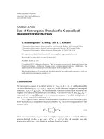
Figure 1: Time evolution of population of ux, y, t and vx, y, t when α 1,β 1ina for 4.4.
Tabl e 1: Comparison of the numerical values with Homotopy perturbation method and Variational
iteration method when a 0.05,b 0.03, and c 0.01 for 1.1,and4.1.
tα β Numerical value u, v by HPM Numerical value u, v by VIM
0.02
1 99.4831,10.614699.4834,10.6323
0.9 99.1865,10.963399.3065,10.8375
0.2
1 93.0910,17.851493.3908,17.7382
0.9 90.5735,20.556792.4584,18.8198
0.3
1 87.9348,23.443088.9466,22.7237
0.9 83.7933,27.778587.8005,24.0532
Then the approximate solution in a series form is
u
x, y, t
u
0
u
1
u
2
u
3
···,v
x, y, t
v
0
v
1
v
2
v
3
···. 4.4
Figure 1 shows the approximate solutions for 4.4 by using the HPM when choosing
the constant initial condition u
0
100,v
0
10 and a 0.05,b 0.03, and c 0.01. From
the figures, it is clear to see the time evolution of prey-predator population density and
we also know that the numerical solutions of fractional prey-predator population model is
continuous with the parameter α and β.
Table 1 shows the approximate solutions of predator-prey system for 1.1 and
initial condition 4.1 by using the Homotopy perturbation method and Variational iteration
method when parameter a 0.05,b 0.03,c 0.01,u
0
100, and v
0
10. It is noted
that only the forth-order of the Homotopy perturbation solution were used in evaluating the
approximate solutions for Table 1 Unlike the Variational iteration method, in this method,
we do not need the Lagrange multiplier, correction functional, stationary conditions, or
calculating integrals, which eliminate the complications that exist in the VIM. So, it is evident
that HPM used in this paper has high accuracy. And from the comparison of the numerical
values with HPM and VIM, we also know that, as the time t and the parameter α, β increase,
the error between the two methods is growing.
Advances in Difference Equations 7
Case 2. In this case, the initial conditions of systems 1.1 are given by
u
x, y, 0
e
xy
,v
x, y, 0
e
xy
. 4.5
By using 3.1 and 3.2, we now successively obtain
u
0
e
xy
,v
0
e
xy
, 4.6
u
1
e
xy
2 a −be
xy
t
α
Γ
1 α
,v
1
e
xy
2 − c be
xy
t
β
Γ
1 β
, 4.7
u
2
e
xy
2 a − be
xy
a − be
xy
2
2 a − 4be
xy
t
2α
Γ
1 2α
−
be
2x2y
2 − c be
xy
t
αβ
Γ
1 α β
,
4.8
v
2
e
xy
2 −c be
xy
be
xy
− c
2
2 −c 4be
xy
t
2β
Γ
1 2β
be
2x2y
2 a − be
xy
t
αβ
Γ
1 α β
,
4.9
u
3
be
2x2y
8 a
c − 2
− b
18 2a c
e
xy
2b
2
e
2x2y
t
2αβ
Γ
1 2α β
e
xy
2 a
2
2 a − b
−
10 2a
8 a − b
be
xy
18 a − b
b
2
e
2x2y
t
3α
Γ
1 3α
−be
2x2y
2 −c
2
b
10 − 2c
e
xy
b
2
e
2x2y
t
α2β
Γ
1 α 2β
Γ
1 α β
−be
2x2y
2 a − be
xy
2 −c be
xy
t
2αβ
Γ
1 α
Γ
1 β
Γ
1 2α β
,
4.10
v
3
be
2x2y
2 a
8 −c
b
a − 18 2c
e
xy
− 2b
2
e
2x2y
t
α2β
Γ
1 α 2β
e
xy
2 − c
2
2 b − c
10 − 2c
8 b − c
be
xy
18 b −c
b
2
e
2x2y
t
3β
Γ
1 3β
be
2x2y
2 a
2
− b
10 2a
e
xy
b
2
e
2x2y
t
2αβ
Γ
1 2α β
Γ
1 α β
be
2x2y
2 a − be
xy
2 −c be
xy
t
α2β
Γ
1 α
Γ
1 β
Γ
1 α 2β
.
4.11
8AdvancesinDifference Equations
40
50
60
70
80
90
0
0.2
0.4
0.6
0.8
1
x a
xis
0
0.5
1
y a
x
i
s
Prey density
a
0
0.2
0.4
0.6
0.8
1
0
0.5
1
x axis
y a
xis
0
20
40
60
80
100
120
Predator density
b
Figure 2: The surface shows the solution of ux, y, t and vx, y, t when α 0.88,β 0.54,a 0.7,b
0.03,c 0.3,t 0.53 in a and c 0.9,t 0.6inb for 4.11.
0
0.2
0.4
0.6
0.8
1
x axis
0
0.5
1
y axi
s
20
30
40
50
60
Prey density
a
Prey density
0
0.2
0.4
0.6
0.8
1
x axis
0
0.5
1
y a
x
i
s
0
10
20
30
40
50
60
b
Figure 3: The surface shows the solution of ux, y, t when α 0.88,β 0.54,c 0.3,t 0.53, a 0.5,b
0.03 in a and a 0.7,b 0.04 in b for 4.11.
Figure 2 shows t he numerical solutions for prey-predator population system with
appropriate parameter. From the figures, we know that prey population density first increases
with the spatial variables, then decreases. although the predator population density always
increase with the spatial variables with the parameter we choose here. Analysis and results
of prey-predator population system indicate that the fractional model match the anomalous
biological diffusion behavior observed in the field.
Figure 3 shows the numerical solutions for prey population density with different
values of parameter a, b, that is, natural birth rate of prey population and competitive rate
between predator and prey population. Comparing Figures 2 and 3, we concluded that the
parameter a, b infects the increase speed, the Maximum value, and the decrease speed of the
prey population. In the same way, the parameter b, c infects predator population growth. This
behavior in agreement with realistic results.
Case 3. We will consider the initial conditions of fractional predator-prey equation 1.1
u
x, y, 0
xy, v
x, y, 0
e
xy
. 4.12
Advances in Difference Equations 9
We now successively obtain by using 3.1 and3.2
u
0
xy, v
0
e
xy
,
u
1
−x
2
− y
2
4ax
2
y
2
− 4be
xy
x
2
y
2
t
α
4xy
√
xyΓ
1 α
,v
1
e
xy
2 −c b
√
xy
t
β
Γ
1 β
,
u
2
a − be
xy
−x
2
− y
2
4ax
2
y
2
− 4be
xy
x
2
y
2
t
2α
4xy
√
xyΓ
1 2α
−
be
xy
√
xy
2 − c b
√
xy
t
αβ
Γ
1 α β
,
√
xy
15y
4
4
a − be
xy
x
2
y
4
16be
xy
x
3
y
4
− x
4
15 4ay
2
4be
xy
y
2
4y − 1
t
2α
16x
4
y
4
Γ
1 2α
,
v
2
e
xy
c
2
b
bxy 2
√
xy
− 2c
1 b
√
xy
t
2β
4xy
√
xyΓ
1 2β
be
xy
−x
2
− y
2
4ax
2
y
2
− 4be
xy
x
2
y
2
t
αβ
4xy
√
xyΓ
1 α β
−
e
xy
−16 8c
xy
√
xy b
y
2
− 4xy
2
x
2
1 − 4y − 8y
2
t
2β
16x
4
y
4
Γ
1 2β
.
4.13
Because of the knowledge of various perturbation methods that low-order approxi-
mate solution leads to high accuracy, there requires no infinite series mostly 2–4 terms a re
enough. The corresponding solutions are obtained according to the recurrence relation using
Mathematica.
5. Conclusion
In this letter, we implement relatively new analytical techniques, the Homotopy perturbation
method, for solving nonlinear fractional partial differential equations arising in prey-predator
biological population dynamics system. Comparing the methodology HPM to ADM, VIM
and HAM have the advantages. Unlike the ADM, the HPM is free from the need to use
Adomian polynomials. In this method we do not need the Lagrange multiplier, correction
functional, stationary conditions, or calculating integrals, which eliminate the complications
that exist in the VIM. In contrast to the HAM, this method is not required to solve the
functional equations in each iteration the efficiency of HAM is very much depended on
choosing auxiliary parameter. We can easily conclude that the Homotopy perturbation
method is an e fficient tool to solve approximate solution of nonlinear fractional partial
differential equations.
10 Advances in Difference Equations
Acknowledgments
The authors thank to the referees for their fruitful advices and comments. This work
was supported partly by the National Science Foundation of Shandong Province Grant
nos. Y2007A06 & ZR2010Al019 and the China Postdoctoral Science Foundation Grant
no. 20100470783.
References
1 I. Podlubny, Fractional Differential Equations, vol. 198 of Mathematics in Science and Engineering,
Academic Press, New York, NY, USA, 1999.
2 R. Metzler and J. Klafter, “The random walks guide to anomalous diffusion: a fractional dynamics
approach,” Physics Reports A, vol. 339, pp. 1–77, 2000.
3 R. Hilfer, Applications of Fractional Calculus in Physics, World Scientific, Singapore, 2000.
4 A. K. Golmankhaneh, A. K. Golmankhaneh, and D. Baleanu, “On nonlinear fractional Klein-Gordon
equation,” Signal Processing, vol. 91, pp. 446–451, 2011.
5 S. Z. Rida, H. M. El-Sherbiny, and A. A. M. Arafa, “On the solution of the fractional nonlinear
Schr
¨
odinger equation,” Physics Letters A, vol. 372, no. 5, pp. 553–558, 2008.
6 X. Y. Jiang and M. Y. Xu, “Analysis of fractional anomalous diffusion caused by an instantaneous
point source in disordered fractal media,” International Journal of Non-Linear Mechanics,vol.41,pp.
156–165, 2006.
7 S. Wang and M. Xu, “Axial Couette flow of two kinds of fractional viscoelastic fluids in an annulus,”
Nonlinear Analysis: Real World Applications, vol. 10, no. 2, pp. 1087–1096, 2009.
8 J H. He, “Homotopy perturbation technique,” Computer Methods in Applied Mechanics and Engineering,
vol. 178, no. 3-4, pp. 257–262, 1999.
9 J H. He, “A coupling method of a homotopy technique and a perturbation technique for non-linear
problems,” International Journal of Non-Linear Mechanics, vol. 35, no. 1, pp. 37–43, 2000.
10 J H. He, “The homotopy perturbation method nonlinear oscillators with discontinuities,” Applied
Mathematics and Computation, vol. 151, no. 1, pp. 287–292, 2004.
11 J. H. He, “Application of homotopy perturbation method to nonlinear wave equations,” Chaos,
Solitons & Fractals, vol. 26, pp. 695–700, 2005.
12 X. Li, M. Xu, and X. Jiang, “Homotopy perturbation method to time-fractional diffusion equation
with a moving boundary condition,” Applied Mathematics and Computation, vol. 208, no. 2, pp. 434–
439, 2009.
13 Q. Wang, “Homotopy perturbation method for fractional KdV-Burgers equation,”
Chaos, Solitons &
Fractals, vol. 35, no. 5, pp. 843–850, 2008.
14 S. Momani and Z. Odibat, “Homotopy perturbation method for nonlinear partial differential
equations of fractional order,” Physics Letters A, vol. 365, no. 5-6, pp. 345–350, 2007.
15 Z. Odibat and S. Momani, “Modified homotopy perturbation method: a pplication to quadratic Riccati
differential equation of fractional order,” Chaos, Solitons & Fractals, vol. 36, no. 1, pp. 167–174, 2008.
16 F. Shakeri and M. Dehghan, “Numerical solution of a biological population model using He’s
variational iteration method,” Computers & Mathematics with Applications, vol. 54, no. 7-8, pp. 1197–
1209, 2007.
17 S. Z. Rida and A. A. M. Arafa, “Exact solutions of fractional-order biological population model,”
Communications in Theoretical Physics, vol. 52, no. 6, pp. 992–996, 2009.
18 Y. Tan, H. Xu, and S J. Liao, “Explicit series solution of travelling waves with a front of Fisher
equation,” Chaos, Solitons & Fractals, vol. 31, no. 2, pp. 462–472, 2007.
19 S. Petrovskii and N. Shigesada, “Some exact solutions of a generalized Fisher equation related to the
problem of biological invasion,” Mathematical Biosciences, vol. 172, no. 2, pp. 73–94, 2001.
20 S. R. Dunbar, “Travelling wave solutions of diffusive Lotka-Vo lterra equations,” Journal of
Mathematical Biology, vol. 17, no. 1, pp. 11–32, 1983.
Advances in Difference Equations 11
21 S. A. Gourley and N. F. Britton, “A predator-prey reaction-diffusion system with nonlocal effects,”
Journal of Mathematical Biology, vol. 34, no. 3, pp. 297–333, 1996.
22 S. Petrovskii, H. Malchow, and B L. Li, “An exact solution of a diffusive predator-prey system,”
Proceedings of The Royal Society of London A, vol. 461, no. 2056, pp. 1029–1053, 2005.
23 A. Kadem and D. Baleanu, “Homotopy perturbation method for the coupled fractional Lotka-Volterra
equations,” Romanian Journal of P hysics, vol. 56, 2011.