Báo cáo hóa học: " Research Article Time-Delay and Fractional Derivatives" doc
Bạn đang xem bản rút gọn của tài liệu. Xem và tải ngay bản đầy đủ của tài liệu tại đây (865.05 KB, 12 trang )
Hindawi Publishing Corporation
Advances in Difference Equations
Volume 2011, Article ID 934094, 12 pages
doi:10.1155/2011/934094
Research Article
Time-Delay and Fractional Derivativ es
J. A. Tenreiro Machado
Department of Electrical Engineering, Institute of Engineering of Porto,
Rua Dr. Ant
´
onio Bernardino de Almeida, 431, 4200-072 Porto, Portugal
Correspondence should be addressed to J. A. Tenreiro Machado,
Received 7 January 2011; Accepted 4 February 2011
Academic Editor: J. J. Trujillo
Copyright q 2011 J. A. Tenreiro Machado. This is an open access article distributed under the
Creative Commons Attribution License, which permits unrestricted use, distribution, and
reproduction in any medium, provided the original work is properly cited.
This paper proposes the calculation of fractional algorithms based on time-delay systems. The
study starts by analyzing the memory properties of fractional operators and their relation with
time delay. Based on the Fourier analysis an approximation of fractional derivatives through time-
delayed samples is developed. Furthermore, the parameters of the proposed approximation are
estimated by means of genetic algorithms. The results demonstrate the feasibility of the new
perspective.
1. Introduction
Fractional calculus FC deals with the generalization of integrals and derivatives to a
noninteger order 1–7. In the last decades the application of FC verified a large development
in the areas of physics and engineering and considerable research about a multitude of
applications emerged such as, viscoelasticity, signal processing, diffusion, modeling, and
control 8–17. The area of dynamical systems and control has received a considerable
attention, and recently several papers addressing evolutionary concepts and fractional
algorithms can be mentioned 18, 19. Nevertheless, the algorithms involved in the
calculation of fractional derivatives require the adoption of numerical approximations 20–
26, and new research directions are clearly needed.
Bearing these ideas in mind, this paper addresses the optimal system control using
fractional order algorithms and is organized as follows. Section 2 introduces the calculation of
fractional derivatives and formulates the problem of optimization through genetic algorithms
GAs.Section3 presents a set of experiments that demonstrate the effectiveness of the
proposed optimization strategy. Finally, Section 4 outlines the main conclusions.
2AdvancesinDifference Equations
2. Problem Formulation and Adopted Techniques
There are several definitions of fractional derivatives. The Riemann-Liouville, the Gr
¨
unwald-
Letnikov, and the Caputo definitions of a fractional derivative of a function ft are given
by
a
D
α
t
f
t
1
Γ
n − α
d
n
dt
n
t
a
f
τ
t − τ
α−n1
dτ, n −1 <α<n,
a
D
α
t
f
t
lim
h →0
1
h
α
t−a/h
k0
γ
α, k
f
t − kh
,
γ
α, k
−1
k
Γ
α 1
α − k 1
,
a
D
α
t
f
t
1
Γ
α − n
t
a
f
n
τ
t − τ
α−n1
dτ, n − 1 <α<n,
2.1
where Γ· is the Euler’s gamma function, x means the integer part of x,andh is the step
time increment.
On the other hand, it is possible to generalize several results based on transforms,
yielding expressions such as the Fourier expression
F
0
D
α
t
f
t
jω
α
F
f
t
−
n−1
k0
jω
k
0
D
α−k−1
t
f
0
, 2.2
where ω and F represent the Fourier variable and operator, respectively, and j
√
−1.
These expressions demonstrate that fractional derivatives have memory, contrary to
integer derivatives that consist in local operators. There is a long standing discussion, still
going on, about the pros and cons of the different definitions. These debates are outside
the scope of this paper, but, in short, while the Riemann-Liouville definition involves
an initialization of fractional order, the Caputo counterpart requires integer order initial
conditions which are easier to apply often the Caputo’s initial conditions are called freely
as “with physical meaning”.TheGr
¨
unwald-Letnikov formulation is frequently adopted in
numerical algorithms because it inspires a discrete-time calculation algorithm, based on the
approximation of the time increment h through the sampling period.
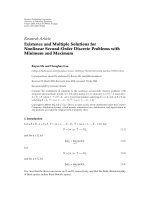
We verify that a fractional derivative requires an infinite number of samples capturing,
therefore, all the signal history, contrary to what happens with integer order derivatives that
are merely local operators 27. This fact motivates the evaluation of calculation strategies
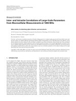
based on delayed signal samples and leads to the study presented in this paper. In this line
of thought we can think in concentrating the delayed samples into a finite number of points
that somehow “average” a given set number of sampling instants see Figure 1.
The concept of time-delayed samples for representing the signal memory can be
formulated analytically as
a
D
α
t
f
t
≈ a
0
f
t
r
k1
a
k
f
t τ
k
, 2.3
Advances in Difference Equations 3
Past
ft − k 1h
ft − kh
ft − k −1h
ft − 2h
ft − h
ft
Future
Present
−γα, 1ft
−γα, 2ft − h
γα, 3ft − 2h
Time
a
Past
ft − τ
k
ft − τ
1
ft
Future
Present
a
k
ft − τ
k
a
1
ft − τ
1
a
0
ft
Time
b
Figure 1: Conceptual diagram of the time delay perspective of the fractional derivative.
where a
k
∈ and τ
k
∈ are weight coefficients and the corresponding delays and r ∈ℵis
the order of the approximation.
Before continuing we must mention that, although based on distinct premises,
expression 2.3, inspired by the interpretation of fractional derivatives proposed in 27,
is somehow a subset of the interesting multiscaling functional equation proposed by
Nigmatullin in 28. Besides, while in 28 we can have complex values, in the present case
we are restricted to real values for the parameters. In fact, expression 2.3 adopts the well-
known time-delay operator, usual in control system theory, following the Laplace expression
L{ft τ
k
} e
τ
k
s
L{ft},wheres and L represent the Laplace variable and operator,
respectively.
Another aspect that deserves attention is the fact that while stability and causality
may impose restrictions to the parameters in 2.3 it was decided not to impose apriori
any restriction to the numerical values in the optimization procedure to be developed in
the sequel. For example, in what concerns the delays, while it seems not feasible to “guess”
the future values of the signal and only the past is available for the signal processing, it is
important to analyze the values that emerge without establishing any limitation apriorito
their values. Nevertheless, in a second phase, the stability and causality will be addressed.
4AdvancesinDifference Equations
0
5
10
15
20
Im
0 5 10 15 20
Re
jw
∧
0.5
r 1
r 2
r 3
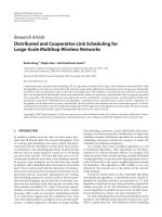
Figure 2: Polar diagram of jω
α
and the approximation a
0
r
k1
a
k
e
jωτ
k
for r {1, 2, 3}, α 0.5, and
ω
max
500.
The development of an algorithm for the calculation of {a
0
,a
k
,τ
k
}, k 1, ,r, given
the approximation and fractional orders r and α, respectively, can be established either in the
time or the frequency domains. In this paper we adopt the Fourier expression 2.2 with null
initial conditions, leading to
F
0
D
α
t
f
t
jω
α
F
f
t
≈ a
0
r
k1
a
k
e
jωτ
k
F
f
t
. 2.4
The parameters a
k
and τ
k
can be optimized in the perspective of the functional
J
r, α
n
i1
jω
α
−
a
0
r
k1
a
k
e
jωτ
k
, 2.5
where i represents an index of the sampling frequencies ω
i
within the bandwidth ω
min
≤
ω
i
≤ ω
max
and n denotes the total number of sampling frequencies. Therefore, the quality
of the approximation depends not only on the orders r and α, but also on the bandwidth
ω
min
≤ ω ≤ ω
max
.
For the optimization of J in 2.5 it is adopted a genetic algorithm GA.GAsarea
class of computational techniques to find approximate solutions in optimization and search
problems 29, 30. GAs are simulated through a population of candidates of size N that
evolve computationally towards better solutions. Once the genetic representation and the
fitness function are defined, the GA proceeds to initialize a population randomly and then
to improve them through the repetitive application of mutation, crossover, and selection
operators. During the successive iterations, a part or the totality of the population is selected
to breed a new generation. Individual solutions are selected through a fitness-based process,
where fitter solutions measured by a fitness function J are usually more likely to be selected.
Advances in Difference Equations 5
10
−1
10
0
10
1
10
2
10
3
a
0
, −a
1
00.10.20.30.40.50.60.70.80.91
α
r 1,a
0
r 1, −a
1
a
0
0.001
0.002
0.003
0.004
0.005
0.006
0.007
−T
1
00.10.20.30.40.50.60.70.80.91
α
r 1, −T
1
b
10
−1
10
0
10
1
10
2
10
3
a
0
, −a
1
, −a
2
00.10.20.30.40.50.60.70.80.91
α
r 2,a
0
r 2, −a
1
r 2, −a
2
c
0
0.005
0.01
0.015
0.02
−T
1
, −T
2
00.10.20.30.40.50.60.70.80.91
α
r 2, −T
1
r 2, −T
2
d
10
−1
10
0
10
1
10
2
10
3
a
0
, −a
1
, −a
2
, −a
3
00.10.20.30.40.50.60.70.80.91
α
r 3, −a
0
r 3, −a
1
r 3, −a
2
r 3, −a
3
e
10
−4
10
−3
10
−2
10
1
10
0
−T
1
,T
2
, −T
3
00.10.20.30.40.50.60.70.80.91
α
r 3, −T
1
r 3, −T
2
r 3, −T
3
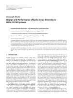
f
Figure 3: Evolution of the approximation parameters and fitness function versus α for r {1, 2, 3} and
ω
max
500.
6AdvancesinDifference Equations
10
0
10
1
10
2
10
3
a
0
00.10.20.30.40.50.60.70.80.91
α
ω 100
ω 200
ω 300
ω 400
ω 500
a
10
−1
10
0
10
1
10
2
10
3
−a
1
00.10.20.30.40.50.60.70.80.91
α
ω 100
ω 200
ω 300
ω 400
ω 500
b
10
−3
10
−2
10
−1
−T
1
00.10.20.30.40.50.60.70.80.91
α
ω 100
ω 200
ω 300
ω 400
ω 500
c
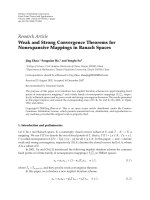
Figure 4: Comparison of the approximation parameters versus α for the bandwidths ω
max
{100, 200, ,
500} and r 1.
The GA terminates when either the maximum number of generations I is produced, or a
satisfactory fitness level has been reached.
The pseudocode of a standard GA is as follows.
1 Choose the initial population
2 Evaluate the fitness of each individual in the population
3 Repeat
a Select best-ranking individuals to reproduce
b Breed new generation through crossover and mutation and give birth to
offspring
c Evaluate the fitness of the offspring individuals
d Replace the worst ranked part of population with offspring
4 Until termination.
Advances in Difference Equations 7
10
−3
10
−2
10
−1
Fitness function
00.10.20.30.40.50.60.70.80.91
α
J, r 1
J, r 2
J, r 3
a
10
−2
10
−1
Fitness function
00.10.20.30.40.50.60.70.80.91
α
J, ω 100
J, ω 200
J, ω 300
J, ω 400
J, ω 500
b
Figure 5: Fitness function versus α for a r {1, 2, 3} and ω
max
500, b the bandwidths ω
max
{100, 200,
,500} and r 1.
A common complementary technique, often adopted to speed-up the convergence,
denoted as elitism, is the process of selecting the better individuals to form the parents in the
offspring generation.
We observe that we have not introduced aprioriany restriction to the numerical values
of the parameters that result during the optimization procedure. It is well known that one of
the advantages of GAs over classical optimization techniques is precisely its characteristic of
handling easily these situations. One technique is simply to substitute “not suitable” elements
of the GA population by new ones generated randomly. Furthermore, during the generation
of the GA elements it is straightforward to impose restrictions. As mentioned previously, in
a first phase it is not considered any limitation in order to reveal more clearly the pattern
that emerges freely with the time-delay algorithm. After having the preliminary results, in a
second phase, several restrictions are considered, and the optimization GA is executed again.
3. Numerical Experiments and Results
In this section we develop a set of experiments for the analysis of the proposed concepts.
Therefore, we study the case of approximation orders and fractional orders r {1, 2, 3} and
α {0.1, 0.2, ,0.9}, respectively. In what concerns the bandwidth are considered ω
min
0, and ω
max
{100, 200, ,500} rad/s.Inallcasesareadoptedn 60 and sampling
frequencies and identical distances between consecutive measuring points along the locus of
jω
α
.
Experiments demonstrated some difficulties in the GA acquiring the optimal values,
being the problem harder the higher the value of r, that is, the larger the number of
parameters to be estimated. Consequently, several measures to overcome that problem were
envisaged, namely, a large GA population with N 2 × 10
4
elements, the crossover of all
population elements and the adoption of elitism, a mutation probability of 10%, and an
evolution with I 10
3
iterations. Even so, it was observed that the GA tended to stabilize
in suboptimal solutions and other values for the GA parameters had no significant impact.
8AdvancesinDifference Equations
0
5
10
15
20
Im
0 5 10 15 20 25
Re
Pade, r 1
Delay, r 1
Ideal
a
0
5
10
15
20
Im
0 5 10 15 20 25
Re
Pade, r 2
Delay, r 2
Ideal
b
0
5
10
15
20
Im
0 5 10 15 20 25
Re
Pade, r 3
Delay, r 3
Ideal
c
Figure 6: Polar diagrams of jω
α
and the approximations 2.4 and 3.3 for r {1, 2, 3}, α 0.5and
0 ≤ ω ≤ 500 rad/s, h 0.005 s.
Therefore, a complementary strategy was taken to prevent such behavior, by restarting the
base GA population and executing new trials until getting a good solution.
It was also observed that all GA executions lead to positive values of a
0
.Inwhat
concerns a
k
and τ
k
, k 1, ,r, it was verified that most experiments lead to negative values;
nevertheless, in some cases, particularly for α near integer values, where the GA had more
convergence difficulties, occasionally some positive values occurred. Several experiments
restricting the GA to negative values proved that the fitting was possible with good accuracy,
and, therefore, for avoiding scattered results with unclear meaning, those restrictions were
included in the optimization algorithm.
Figure 2 shows a typical case, namely, the polar diagram of jω
α
and the approxima-
tion a
0
r
k1
a
k
e
jωτ
k
for r {1, 2, 3}, α 0.5, and ω
max
500.
Figure 3 shows the evolution of the approximation parameters and fitness function
versus α,forr {1, 2, 3}, ω
max
500. Figure 4 compares the cases of increasing bandwidth
ω
max
{100, 200, ,500} for r 1.
Advances in Difference Equations 9
−200
−150
−100
−50
0
50
100
Roots
00.10.20.30.40.50.60.70.80.91
α
r 1
r 2
r 3
Figure 7: Roots of the characteristic equation of approximation 2.4 versus α for r {1, 2, 3}.
Figure 5 depicts the variation of the fitness function J for different orders of
approximation and for different bandwidths.
It is clear that the higher the value of r, the better the approximation, that is, the smaller
the value of J. When the bandwidth increases we observe larger values of the weighting
factors a
k
,butthedelaysτ
k
remain in a limited range a small values, being more close/apart
to/from zero for values of α near/far the unit. Moreover, for larger bandwidths the GA has
more difficulties in estimating the parameters of the approximation.
While the primary goal of this paper is to explore the relationship between the
fractional derivative and the time-delay operators, it is interesting to compare the results of
the present approach with those of classical approximations. In this perspective, we consider
the discrete time domain and the Euler and Tustin rational expressions, H
0
z
−1
1/h1 −
z
−1
and H
1
z
−1
2/h1 − z
−1
/1 z
−1
,wherez represents the Z transform operator
and h the sampling period. These expressions are also called generating approximants of zero
and first order, respectively, and their generalization to a noninteger order α yields
s
α
≈
1
h
1 − z
−1
α
H
α
0
z
−1
,
s
α
≈
2
h
1 − z
−1
1 z
−1
α
H
α
1
z
−1
.
3.1
Weighting H
α
0
z
−1
and H
α
1
z
−1
by the factors p and 1 − p leads to the average
H
av
z
−1
;
p, α
pH
α
0
z
−1
1 − p
H
α
1
z
−1
. 3.2
10 Advances in Difference Equations
The so-called Al-Alaoui operator corresponds to an interpolation of H
α
0
z
−1
and H
α
1
z
−1
with weighting factor p 3/4 31–33. Often it is adopted a Pad
´
e expansion of order r ∈ℵin
the neighborhood of z 0, leading to a rational fraction of the type
H
k
z
−1
r
i0
a
i
z
−i
r
i0
b
i
z
−i
,a
i
,b
i
∈ . 3.3
Figure 6 compares the frequency response of the proposed algorithm 2.4 and the fraction
3.3,withp 3/4andh 0.005 s, for 0 ≤ ω ≤ 500rad/s and the orders r {1, 2, 3}, α 0.5.
It is clear that expression 2.4 leads to a superior approximation. Furthermore,
although not particularly important with present day computational resources, expression
2.4 poses a calculation load which is inferior to the one of 3.3.Infact,sinceinrealtime
the delay consists simply in a memory shift, we have r versus 2r sums and r versus 2r 1
multiplications for 2.4 and 3.3, respectively.
The stability of the resulting expression is also important. Figure 7 depicts the roots of
the characteristic equation of approximation 2.4 versus α for r {1, 2, 3}.Weverifythatwe
may have stability problems near integer values of α.
In conclusion, while the aim of this paper was to explore the relationship between the
fractional operator and the time delay, it was verified that the proposed algorithm can be
applied to successfully approximate fractional expressions.
4. Conclusions
The recent advances in FC point towards important developments in the application of
this mathematical concept. During the last years several algorithms for the calculation
of fractional derivatives were proposed, but the fact is that the results are still far from
the desirable. In this paper, a new method, based on the intrinsic properties of fractional
systems, that is, inspired by the memory effect of the fractional operator, was introduced.
The optimization scheme for the calculation of fractional approximation adopted a genetic
algorithm, leading to near-optimal solutions and to meaningful results. The conclusions
demonstrate not only the goodness of the proposed strategy, but point also towards further
studies in its generalization to other classes of fractional dynamical systems and to the
evaluation of time-based techniques.
Acknowledgment
The author would like to acknowledge FCT, FEDER, POCTI, POSI, POCI, POSC, POTDC,
and COMPETE for their support to R&D Projects and GECAD Unit.
References
1 K. B. Oldham and J. Spanier, The Fractional Calculus: Theory and Applications of Differentiation and
Integration to Arbitrary Order, Academic Press, London, UK, 1974.
2 K. S. Miller and B. Ross, An Introduction to the Fractional Calculus and Fractional Differential Equations,
A Wiley-Interscience Publication, John Wiley & Sons, New York, NY, USA, 1993.
3 S. G. Samko, A. A. Kilbas, and O. I. Marichev, Fractional Integrals and Derivatives: Theory and
Applications, Gordon and Breach Science Publishers, Yverdon, Switzerland, 1993.
Advances in Difference Equations 11
4 I. Podlubny, Fractional Differential Equations: An Introduction to Fractional Derivatives, Fractional
Differential Equations, to Methods of Their Solution and Some of Their Applications, vol. 198 of Mathematics
in Science and Engineering, Academic Press, San Diego, Calif, USA, 1999.
5 A. A. Kilbas, H. M. Srivastava, and J. J. Trujillo, Theory and Applications of Fractional Differential Equa-
tions, vol. 204 of North-Holland Mathematics Studies, Elsevier Science, Amsterdam, The Netherlands,
2006.
6 M. Klimek, On Solutions of Linear Fractional D ifferential Equations of a Variational Type,Czestochowa
University of Technology, 2009.
7 K. Diethelm, TheAnalysisofFractionalDifferential Equations: An Application-Oriented Exposition Using
Differential Operators of Caputo Type, vol. 2004 of Lecture Notes in Mathematics, Springer, Berlin,
Germany, 2010.
8 A. Oustaloup, La commande CRONE: commande robuste d’ordre non entier, Hermes, 1991.
9 R. R. Nigmatullin, “A fractional integral and its physical interpretation,” Teoreticheskaya i Matematich-
eskaya Fizika, vol. 90, no. 3, pp. 354–368, 1992.
10 I. Podlubny, “Fractional-order systems and PI
λ
D
μ
-controllers,” IEEE Transactions on Automatic Control,
vol. 44, no. 1, pp. 208–214, 1999.
11 J. A. Tenreiro Machado, “Discrete-time fractional-order controllers,” Fractional Calculus & Applied
Analysis, vol. 4, no. 1, pp. 47–66, 2001.
12 R. L. Magin, Fractional Calculus in Bioengineering, Begell House Publishers, 2006.
13 J.Sabatier,O.P.Agrawal,andJ.A.TenreiroMachad,Eds.,Advances in Fractional Calculus: Theoretical
Developments and Applications in Physics and Engineering, Springer, Dordrecht, The Netherlands, 2007.
14 D. Baleanu, “About fractional quantization and fractional variational principles,” Communications in
Nonlinear Science and Numerical Simulation, vol. 14, no. 6, pp. 2520–2523, 2009.
15 F. M ainardi, Fractional Calculus and Waves in Linear Viscoelasticity: An Introduction to Mathematical
Models, Imperial College Press, London, UK, 2010.
16 R. Caponetto, G. Dongola, L. Fortuna, and I. Petr
´
a
ˇ
s, Fractional Order Systems: Modeling and Control
Applications, World Scientific, 2010.
17 C.A.Monje,Y.Q.Chen,B.M.Vinagre,D.Xue,andV.Feliu,Fractional Order Systems and Controls:
Fundamentals and Applications, Advances in Industrial Control, Springer, Berlin, Germany, 2010.
18 J. A. Tenreiro Machado, A. M. Galhano, A. M. Oliveira, and J. K. Tar, “Optimal approximation of
fractional derivatives through discrete-time fractions using genetic algorithms,” Communications in
Nonlinear Science and Numerical Simulation, vol. 15, no. 3, pp. 482–490, 2010.
19 J. A. Tenreiro Machado, “Optimal tuning of fractional controllers using genetic algorithms,” Nonlinear
Dynamics, vol. 62, no. 1-2, pp. 447–452, 2010.
20 M. A. Al-Alaoui, “Novel digital integrator and differentiator,” Electronics Letters,vol.29,no.4,pp.
376–378, 1993.
21 J. A. Tenreir Machado, “Analysis and design of fractional-order digital control systems,” Systems
Analysis Modelling Simulation, vol. 27, no. 2-3, pp. 107–122, 1997.
22 C C. Tseng, “Design of fractional order digital FIR differentiators,” IEEE Signal Processing Letters,vol.
8, no. 3, pp. 77–79, 2001.
23 Y. Q. Chen and K. L. Moore, “Discretization schemes for fractional-order di
fferentiators and
integrators,” IEEE Transactions on Circuits and Systems. I, vol. 49, no. 3, pp. 363–367, 2002.
24 B. M. Vinagre, Y. Q. Chen, and I. Petr
´
a
ˇ
s, “Two direct Tustin discretization methods for fractional-order
differentiator/integrator,” Journal of the Franklin Institute, vol. 340, no. 5, pp. 349–362, 2003.
25 Y. Chen and B. M. Vinagre, “A new IIR-type digital fractional order differentiator,” Signal Processing,
vol. 83, no. 11, pp. 2359–2365, 2003.
26 R. S. Barbosa, J. A. Tenreiro Machado, and M. F. Silva, “Time domain design of fractional
differintegrators using least-squares,” Signal Processing, vol. 86, no. 10, pp. 2567–2581, 2006.
27 J. A. Tenreiro Machado, “Fractional derivatives: Probability interpretation and frequency response of
rational approximations,” Communications in Nonlinear Science and Numerical Simulation, vol. 14, no.
9-10, pp. 3492–3497, 2009.
28 R. R. Nigmatullin, “Strongly correlated variables and existence of the universal distribution function
for relative fluctuations,” Physics of Wave Phenomena, vol. 16, no. 2, pp. 119–145, 2008.
29 J. H. Holland, Adaptation in Natural and Artificial Systems: An Introductory Analysis with Applications to
Biology, Control, and Artificial Intelligence, University of Michigan Press, Ann Arbor, Mich, USA, 1975.
30 D. E. Goldenberg, Genetic Algorithms in Search Optimization, and Machine Learning, Addison-Wesley,
Reading, Mass, USA, 1989.
12 Advances in Difference Equations
31 M. A. Al-Alaoui, “Novel digital integrator and differentiator,” Electronics Letters,vol.29,no.4,pp.
376–378, 1993.
32 M. A. Al-Alaoui, “Filling the gap between the bilinear and the backward-difference transforms: an
interactive design approach,” International Journal of Electrical Engineering Education, vol. 34, no. 4, pp.
331–337, 1997.
33 J. M. Smith, Mathematical Modeling and Digital Simulation for Engineers and Scientists, Wiley-
Interscience, New York, NY, USA, 1977.