Optical Fiber Communications and Devicesan incorrectly Part 12 pot
Bạn đang xem bản rút gọn của tài liệu. Xem và tải ngay bản đầy đủ của tài liệu tại đây (805.14 KB, 25 trang )
Optical Fiber Communications and Devices
264
of nodes. Dynamic (or online) lightpath establishment considers the case where connection
requests arrive at random time instants, over a prolonged period of time, and are served
upon their arrival, on a one-by-one basis. We focus our study on the online RWA problem.
4.1 RWA algorithm with full flexibility
The proposed multi-cost RWA algorithm consists of two phases. In contrast to traditional
single-cost approach, where each link is characterized by a scalar, in the multi-cost approach
a vector of cost parameters is assigned to each link, from which the parameter vectors of
candidate lightpaths are calculated. In our work, we assume that nodes are equipped with
TSPs that can be tuned to transmit and receive at any wavelength (widely tunable TSPs). In
particular, the number of TSPs each node n is equipped with, depends on its degree D
n
. The
number of TSPs of node n, that are assigned to each link l is assumed to be constant and
equal to T and as a result node n has a total of
nn
TDT
TSPs.
4.1.1 Computing the cost vector of a path
We consider a WDM network with N nodes and L fiber-links, each of which carries m
wavelengths. Each fiber is able to support a common set C={λ
1
, λ
2
,…, λ
m
} of W distinct
wavelengths. The WDM network employs no wavelength conversion. We also assume that
the node where the algorithm is executed (in a decentralized or centralized architecture) has
a picture of the wavelengths’ utilization of all links. Although the algorithm may run in a
decentralized way, and thus due to propagation delays utilization information might be
outdated, we will not focus on such problems. We assume that all nodes are fully flexible
(colorless/directionless nodes) without add/drop constraints.
Cost vector of a link
Each link l is assigned a cost vector that contains m+1 cost parameters:
i. the length L
l
of the link(scalar);
ii. the availability of wavelengths in the form of a Boolean vector
l
W =(w
l1
, w
l2
, ,w
lm
),
whose
i
th
element w
lm
is equal to 0 (false) if wavelength λ
i
is used and equal to 1 (true)
when
λ
i
is free.
Thus, the cost vector characterizing a link
l is given by
V
l
= (L
l
,
l
W
)
Cost vector of a path
Similarly to a link, a path has a cost vector with m+1 parameters, in addition to the list of
labels of the links that comprise the path. Assume a path
p with cost vector
V
p
= (L
p
,
p
W , *p),
where L
p
, and
p
W are as previously described, and *p is the list of identifiers of the links that
comprise path p. The cost vector of p can be calculated by the cost vectors of the links
l=1,2, ,k, that comprise it as:
A Comparative Study of Node Architectures with Add/Drop Constraints in WDM Networks
265
1
1
(1,2, , )
,
,
&
k
k
l
l
l
l
p
k
W
L
V
,
where the operator & denotes the bitwise AND operation. Note that all operations between
vectors have to be interpreted component-wise.
Checking if the path is further extendable
We check if path
p has at least one available wavelength.
If
0
p
W
(all zero vector), then path p is rejected.
Domination relationship
We also define a domination relationship between two paths that can be used to reduce the
number of paths considered by the RWA algorithm. In particular, we will say that
p
1
dominates p
2
(notation: p
1
> p
2
) iff
12 1 2
and
pp p p
LL WW
The “
” relationship for vectors W , should be interpreted component-wise. A path that is
dominated by another path has larger length and worse wavelength availability than the
other path and there is no reason to consider it or extend it further.
4.1.2 Multi-cost RWA algorithm
The proposed multi-cost RWA algorithm consists of two phases:
Phase 1: Computing the set of non-dominated paths P
n-d
The algorithm that computes the non-dominated paths from a given source to all network
nodes (including the destination) can be viewed as a generalization of Dijkstra’s algorithm
that only considers scalar link costs. The basic difference is that instead of a single path, a set
of non-dominated paths between the origin and each node is obtained. Thus a node for
which one path has already been found is not finalized (as in the Dijkstra case), since we can
find more “non-dominated” paths to that node later. An algorithm for obtaining the set
P
n-d
of non-dominated paths from a given source to all nodes is given in (Varvarigos et al., 2008).
By definition, for the given source and destination, the non-dominated paths that the
algorithm returns have at least one available wavelength.
Phase 2: Choosing the optimal lightpath from P
n-d
In the second phase of the proposed algorithm we apply an optimization function or policy
g(V
p
) to the cost vector, V
p
, of each path p
P
n-d
. The function g yields a scalar cost per path
and wavelength (per lightpath) in order to select the optimal one. Given the connections
already established, we order the wavelengths in decreasing utilization order and choose
the lightpath whose wavelength is most used. This approach is the well known “most used
wavelength” algorithm (Zang et al., 2000), proven to exhibit good network–layer blocking
assuming ideal physical layer. In the end, the algorithm establishes the decided lightpath if
there are available transponders (TSPs) in the source/destination nodes of the connection,
assuming colorless/directionless node architectures.
Optical Fiber Communications and Devices
266
4.2 RWA algorithm with limited flexibility
A network topology is represented by a connected graph
G=(V,E). V denotes the set of
OXCs-nodes.
4.2.1 Colored vs. colorless architecture
Colored add/drop ports in network nodes limit the flexibility of the RWA algorithm,
mainly regarding which channels/wavelengths it can use for serving a connection request.
This is because the node ports are permanently assigned to specific wavelengths. In this
case, the links’ wavelength availability vectors
l
W , used by the RWA algorithm, are
updated according to these wavelengths. If the algorithm cannot find a lightpath for serving
a connection request, then manual intervention can be performed. In particular, manual
intervention corresponds to the assignment of an available TSP to a different port than the
one already provisioned. If no TSPs are available, then the demand is finally blocked.
Figure 5a shows how the definition of the wavelength availability vector
l
W of link l has to be
modified to account for the color related constraints. If node
d is the destination of a
connection request, then the availability vectors of the node’s incoming links are modified
according to its available receivers - drop ports (that are tuned to specific wavelengths). For
example in Figure 5a, the original vector of link
l is
0 1 1 1 1
l
W , implying that the available
p
W
0 1 1 1 1
l
W
p
W
l
W
,
0 0 1 0 0
l
W
,l
W
1 1 1 0 1
l
W
,
1 0 0 0 0
l
W
Fig. 5. a) Availability vectors of the RWA algorithm when considering colored ports.
Receivers / drop ports
R
1
, R
3
can only receive wavelengths w
1
, w
3
, respectively.
b) Availability vectors of the RWA algorithm when considering directed ports, where
transmitter / input port T
1
can only send traffic to link l
1
and transmitter / input port T
2
can
only send traffic to link
1
2
.
A Comparative Study of Node Architectures with Add/Drop Constraints in WDM Networks
267
wavelengths of link
l are the
2345
,,,wwww (the example assumes five wavelengths per
fiber). In case the RWA algorithm attempts to find a lightpath that terminates at node
d, then
all the availability vectors of the links incoming to
d are modified based on the way node’s d
drop ports are colored. In our example, node
d can only receive on wavelengths
13
,ww
because only receivers / drop ports
R
1
and R
3
are available and therefore, the original
availability vector is updated to
,
0 0 1 0 0
l
W
. This means that only wavelength
3
w
of link l
is actually available for use by the RWA algorithm in order to end the lightpath in node
d.
If the RWA algorithm cannot find a lightpath, either due to the unavailability of a path
and/or wavelength from source to destination or due to the color constraint, manual
intervention is necessary. In this case the RWA algorithm is re-executed for deciding the
lightpath that will serve the request, assuming that there are not color constraints. Next,
based on the RWA algorithm’s decisions manual intervention is performed so as to plug a
TSP at the decided (input or output) port. As mentioned, the RWA algorithm (that does not
consider color constraints) is executed only if there are free TSPs at the source and
destination nodes of the connection request; otherwise the connection is blocked.
4.2.2 Directed vs. directionless architecture
Colored Non-Directionless ports limit the routing choices available to the RWA algorithm,
mainly regarding the first and the last link of the path to be used for serving a connection.
For example, assume there is only one free input port (with a plugged TSP) connected to a
specific fiber in a node
s. This free input port can only be used by a connection request,
which originates from s and uses this fiber as its first hop. This constraint must be accounted
for by the corresponding RWA algorithm. If a lightpath cannot be found, the connection is
either blocked, or manual intervention is performed to connect an available TSP to another
fiber. In this case, an RWA algorithm that does not consider direction-related constraints
will point out which fiber-link is most efficient to use. In the case where there are no
available TSPs then the connection will be blocked.
In Figure 5b, if node s is the source of a connection request, then we can only set up a
connection from transmitter / input port T
1
to link l
1
and from T
2
to l
2
. Also, the wavelength
availability vectors of the links are again modified, in a way similar to that used for colored
ports. In case we also have color constraints (that is, the ports are not colorless), the RWA
algorithm will have to find a solution under both constraints.
5. TSP assignment policy
An important factor affecting network efficiency in case colored node architectures are used,
is the way the transponders (TSPs) of a link are provisioned to specific wavelengths. Next,
we present a number of such TSP assignment policies.
In Figure 6, we illustrate an abstraction of node architectures based on the configuration of
add/drop ports. Also in this figure we depict the way the TSPs are connected to the optical
fibers (in which wavelength and direction). For example, Fig. 6a presents four add/drop
ports connected statically to Fibers 1 and 2 and wavelengths 1 and 2 respectively, while Fig.
6d presents four add/drop ports that can switch on the fly to any of the two fibers, serving
any wavelength.
Optical Fiber Communications and Devices
268
Fig. 6. a) Different node architectures: a) colored/non-directionless, b) colored/non-
directionless, c) colored/directionless, d) colorless/directionless. Tx,y express the ability of
add/drop port: x is the fiber and y is the wavelength that the transponder (TSP) is plugged
in. The symbol ‘*’ denotes that there is no limitation.
5.1 Colored architectures - policy 1: Lowest wavelength count first
The provision of wavelengths in the TSPs of a link can be performed according to the
“lowest available wavelength count first” rule. That is, assuming there are T available TSPs
per link and no connections are already established, the TSPs can be provisioned to the first
T wavelengths of the link (Figure 6a and 6b). This is the simplest TSP assignment policy that
can be used in colored architectures.
5.2 Colored/directed architecture - policy 2: Cyclic wavelength rotation
In this policy, the T available TSPs of each link are provisioned based on a cyclic rotation
process. That is, the TSPs of the first link of a node are provisioned to wavelengths 1 to
T,
the TSPs of the second link are provisioned to wavelengths T+1 to 2T, and the provisioning
procedure continues similarly to the remaining links, until all the TSPs are provisioned
(Figure 7a). The sense behind this policy is that the available TSPs of a node have to be
provisioned in as many wavelengths as possible, so as each connection
originating/terminating from/to that node to be able to use all the available wavelengths.
5.3 Colored/directionless architecture - policy 2: Full wavelength cover
Under this policy (Figure 7b), all the available TSPs of a node are provisioned to
wavelengths 1 to
nn
TDT
, assuming
n
TW
. In case
n
TW
, then
/
n
TW
TSPs are
A Comparative Study of Node Architectures with Add/Drop Constraints in WDM Networks
269
provisioned to all the wavelengths and the remaining
mod
n
TW
TSPs are provisioned to
wavelengths 1 to mod
n
TW. This policy has the same logic as the previous and also taking
into advantage the directionless feature of the node.
Fig. 7. TSP assignment policy 2 for: (a) the colored/directed architecture, (b) the
colored/directionless architecture (as opposed to policy 1 in Fig. 6a and 6b)
6. Simulation results
The network topology used in our simulations was the generic Deutsche Telekom network
(DTnet) that has 14 nodes and 23 links (Fig. 8). The capacity of a wavelength was assumed
equal to 10Gbps. We performed two different sets of simulations: In the first set, we have
limited resources and we report on blocking performance, while in the second set we have
enough resources to establish all the requested connections and we report on required
manual interventions.
6.1 Impact of node flexibilities in blocking probability
In this set of simulations, connection requests (each requiring bandwidth equal to 10Gbps)
are generated according to a Poisson process with rate
λ (requests/time unit). The source
and destination of a connection are uniformly chosen among the nodes of the network. The
duration of a connection is given by an exponential random variable with average 1/
μ (time
units). Thus, λ/μ gives the total network load in Erlangs. In this set we also assumed that
widely tunable TSPs are plugged into specific ports, while the number of TSPs is constant
during the network operation. That is, we cannot add extra TSPs and if a connection cannot
be served due to limited resources then it is blocked.
In Fig. 9 we examine the performance of the various TSP assignment policies proposed in
conjunction with the node’s architectures considered, assuming network load equal to 100
Optical Fiber Communications and Devices
270
Fig. 8. DT network: 14 nodes, 23 links
Fig. 9. Blocking probability vs. number of transponders when no manual interventions are
allowed, assuming 14 available wavelengths per link and network load equal to 100, for
various node architectures and TSP assignment policies
Erlangs and 14 available wavelengths. We assumed that no MIs are allowed and as a result if
the wavelength of the transmitter (source) does not fit with the wavelength at the receiver
(destination), then the connection is blocked. We observe that the colored/directed and
colored/directionless architectures exhibit the same, bad performance when the TSP
A Comparative Study of Node Architectures with Add/Drop Constraints in WDM Networks
271
assignment policy 1 is used. This is due to the fact that under this policy not all the available
wavelengths are actually utilized. On the other hand the performance of these architectures,
and especially that of the colored/directionless architecture, is improved when TSP
assignment policy 2 is used. Colorless/directed architecture exhibits similar performance with
the most flexible architecture (colorless/directionless) and this can be explained by the
characteristics of the DT network. In particular, the average node degree of DT network is
small and as result the direction related constraint is not as restrictive as the color related one.
Fig. 10 illustrates the blocking probability versus the number of TSPs per link for different
number of available wavelengths. We assume that each fiber has the same number of
wavelengths and TSPs. In the cases where we do not have fully flexible architecture and an
available TSP has to be assigned to a different port than the one originally assigned, so as to
serve a new connection, then a manual intervention is performed, for changing the direction
and the color of a port. For this reason the results of blocking probability presented in Fig. 10
hold for all the node architectures under consideration. Small variations in blocking
probability is possible, because in different architectures the differences in ports flexibilities
lead to different wavelength assignment by the RWA algorithm, which assigns the
wavelengths based on the already provisioned TSPs.
In general, the performance of the RWA algorithm is constrained by the number of
transponders; however, as this number increases, then the number of wavelengths becomes
the performance bottleneck. In particular, we note that in order to achieve zero blocking
probability 8 TSPs and 14 wavelengths per link/fiber are required. When having only 10
available wavelengths per fiber, we cannot achieve zero blocking for load equal to 100
Erlangs, irrespectively of the number of TSPs.
0,00E+00
5,00E-02
1,00E-01
1,50E-01
2,00E-01
2,50E-01
3,00E-01
3,50E-01
4,00E-01
4,50E-01
246810
blocking probability
number of transponders per link (T)
w=10
w=12
w=14
w=16
Fig. 10. Blocking probability vs. number of transponders for different number of available
wavelengths per link, assuming network load equal to 100. Blocking probability is the same
irrespective of the node architecture used.
6.2 Impact of node flexibilities in operational cost
In this study we evaluate a realistic operational scenario of the DT core network. Initially,
we assumed that in year 2008, 270 demands were present. For the year 2008, the network
Optical Fiber Communications and Devices
272
was provisioned with 460 transponders. We made the assumption that new demands arrive
during the next years leading to an increase of 50% in the requested connections per year. In
this set of simulations we allow manual interventions in order to change the port of an
already installed TSP or to install new TSPs.
We define two different types of manual interventions. The type 1 of manual intervention is
the switching of an available transponder from one to another port of the same node.
Manual intervention of type 2 is referred to the installation of extra transponders. We
consider different pre-provisioning strategies (manual interventions of type 2). All strategies
start with 10 TSPs per link, which results in 460 TSPs in total. The first strategy is when there
are no more TSPs available at a particular node to establish a connection, and only a new
TSP is installed. We call this approach one TSP. In the other approaches a certain amount of
TSPs are installed per link (bank of transponders). For example in case of one TSP per link,
we will install 3 extra transponders if the node degree is 3. We have also similar approaches
with 5, 7 and 9 TSPs per link.
In Fig. 11, we show the sum of the manual interventions of type 1 (MI1) and those of type 2
(MI2) cumulated over three years. The results for different node flexibilities are depicted to
point the differences between them. In Fig. 11a) we can observe that provisioning of more
transponders has only a little impact on the amount of manual interventions. In Fig. 11b),
the architecture with the directionless feature is depicted with TSP assignment policy 2. This
results in a lower number of manual interventions as compared to the previous architecture.
In Fig. 11c), it is clear that provisioning of more transponders has huge impact on the
manual interventions. The difference between three and nine transponders per link is really
small. So there is no reason to provision more than 3 transponders per time because the cost
will be increased. In Fig. 11d), we consider the colorless/directionless architecture, which
has the best performance in terms of MIs because all transponders provisioned in the node
can be used for every new demand. There are no constraints in terms of color or fiber
anymore. When provisioning only one TSP per link instead of one TSP, the MIs are
decreased from 270 to 100.
Based on these remarks we are interested in the operational processes that involve several
actions/activities that need to be performed by the operator’s staff. The duration of the
activity determines, to an important extent, the cost of the action. The costs for transport
(going to the location of the node where an intervention is needed) are calculated from the
topology characteristics. We assume that technical teams are present on average 2 links
away from one another, this is every 340 km. The average distance to the failure location is
therefore 85 km. One way and return adds to 170 km, with an average speed of 50 km/h,
this means 3.4 hours for transport.
With the number of MI1 and MI2 (Fig. 11) we can calculate the total transport time and the
real intervention time that is the time to switch a transponder in case of MI1 and the time to
install new transponders in case of MI2. The duration of transport is 3.4 hours and the
duration of switching/installing a transponder is 1 hour.
In Fig. 12 we depict the working hours over the years from 2009 to 2011 needed for manual
intervention purposes. In this figure we present two blocks for the node architectures, where
in the first block we assume that one TSP is installed, while in the second three TSPs per link
are installed. We can see that the colored/directed node and the colored/directionless node
A Comparative Study of Node Architectures with Add/Drop Constraints in WDM Networks
273
0
50
100
150
200
250
300
350
400
450
500
2008 2009 2010 2011
Manual Int erventions
Year
a)
one TSP
one TSP per link
three TSPs per link
five TSPs per link
seven TSPs per link
nine TSPs per link
0
50
100
150
200
250
300
350
400
450
500
2008 2009 2010 2011
Manual Interventions
Year
b)
oneTSP
one TSP per link
three TSPs per link
five TSPs per link
seven TSPs per link
nine TSPs per link
0
50
100
150
200
250
300
350
400
450
500
2008 2009 2010 2011
Manual Interventions
Year
c)
oneTSP
one TSP per link
three TSPs per link
five TSPs per link
seven TSPs per link
nine TSPs per link
0
50
100
150
200
250
300
350
400
450
500
2008 2009 2010 2011
Manual Interventions
Year
d)
oneTSP
one TSP per link
three TSPs per link
five TSPs per link
seven TSPs per link
nine TSPs per link
Fig. 11. Cumulative sum of number of manual interventions for a) colored/directed (TSP
policy 2), b) colored/directionless (TSP policy 2), c) colorless/directed and d)
colorless/directionless.
Optical Fiber Communications and Devices
274
0
200
400
600
800
1000
1200
1400
1600
1800
2000
hours
intervention
transport
one TSP
three TSPs per link
Fig. 12. Working hours of manual interventions
have little improvement in transport times but the intervention times are worst. This
happens because when installing more TSPs at once maybe additional MIs of type 1 will be
necessary to switch a TSP in different port. The improvement of working hours in case of
colorless/directed and colorless/directionless is obvious when installing three TSPs per link
instead of one TSP at once, and this happens because of the saving in transport time.
The colorless/directed architecture has almost the same performance as the colorless
directionless with the provisioning of 3 TSPs per fiber. The benefits of the directionless
architectures are almost negligible due to higher cost and because similar performance can
be achieved with directed architectures when appropriate provision strategies and TSP
assignment policies are used.
7. Conclusion
We evaluated and compared the performance of several node architectures with color and
direction related constraints used in a WDM network. In comparing the node architectures,
we also proposed an adaptation of an RWA algorithm that accounts for the lack of node
flexibility, and aims at achieving performance similar to that obtained with fully flexible
node architectures. Our results demonstrated that in topologies where the node degree is
small, the colored constraint is a more dominant performance limiting factor than the
direction related one. In addition, we observed that even if a sufficient number of
transponders exist in each node, a small number of wavelengths can also be a bottleneck of
A Comparative Study of Node Architectures with Add/Drop Constraints in WDM Networks
275
the network’s performance. Finally, we illustrated that the way and the number of
transponders are assigned to wavelengths are important and assignment policies utilizing
all the available wavelengths should be used.
8. References
Christodoulopoulos, K., et al. (2009). A Multicost Approach to Online Impairment-Aware
RWA,
Proceedings of ICC, 2009
Homa, J & Bala K., (2008). ROADM architectures and their enabling WSS technology,
IEEE
Communications Magazine
, vol. 46, no. 7, pp. 150 –154, 2008
Kaman, V.; Helkey, R. & Bowers, J. (2007) “Multi-degree ROADM’s with agile add-drop
access”,
Proceedings of Photonics in Switching conference, San Francisco (US), Aug.
2007
Keyworth, B., (2005) “ROADM subsystems and technologies”,
Proceeding of OFC/NFOEC
2005 Optical Fiber communication/National Fiber Optic Engineers Conference
,, Vol. 3,
pp. 1–4, 2005
Mezhoudi, M., et al. (2006), “The value of multiple degree ROADMs on metropolitan
network economics”,
Proceeding of OFC/NFOEC 2008 Optical Fiber
communication/National Fiber Optic Engineers Conference
, pp. 1–8, 2006
Ramaswami, R. & Sivarajan K., (1995). Routing and Wavelength Assignment in All-Optical
Networks, IEEE/ACM Transactions on Networking, vol. 3, no. 5, pp. 489-500, Oct.
1995
Ramaswami, R. & Sivarajan K., (2001). Optical Networks: A Practical Perspective, 2nd ed.,
Morgan Kaufmann, 2001
Roorda, P. & Collings B. (2008). Evolution to colorless and directionless roadm architectures,
Proceeding of OFC/NFOEC 2008 Optical Fiber communication/National Fiber Optic
Engineers Conference
, 2008
Saradhi, C. & Subramaniam, S. (2009). Physical layer impairment aware routing (PLIAR) in
WDM optical networks: issues and challenges,
IEEE Communications Surveys &
Tutorials,
Vol. 11, No. 4, pp.109-130
Shen, G.; Bose, S.; Cheng, T.; Lu, C. & Chai T. (2003). The impact of the number of add/drop
ports in wavelength routing all-optical networks,
Optical Networks Magazine, pp.
112–122, 2003
Staessens, D.; Colle, D.; Pickavet, M. & Demeester, P. (2010). Impact of node directionality
on restoration in translucent optical networks,
Proceedings of Optical Communication
(ECOC), 2010 36th European Conference and Exhibition
, 2010.
Turkcu O. & Subramaniam S. (2009). Performance of optical networks with limited
reconfigurability,
IEEE/ACM Transactions on Networking, Vol. 17, No. 6, pp. 2002 -
2013, 2009
Varvarigos E.; Sourlas V. & Christodoulopoulos K. (2008). Routing and Scheduling
Connections in Networks that Support Advance Reservations,
Computer Networks
(58), 2008.
Zang H.; Jue, J. & Mukherjee, B. (2000). A Review of Routing and Wavelength Assignment
Approaches for Wavelength-Routed Optical WDM Networks,
Optical Networks
Magazine
, Vol. 1, 2000
Optical Fiber Communications and Devices
276
Zhu, H. & Mukherjee B. (2005). Online connection provisioning in metro optical WDM
networks using reconfigurable OADMs (ROADMs), IEEE/OSA Journal of Lightwave
Technology
, Vol 23, No. 10, pp. 2893–2901, 2005.
13
Accurate Receiver Model for Optical
Fiber Systems with Polarization
Induced Performance Degradation
Aurenice Oliveira
Michigan Technological University
USA
1. Introduction
Polarization-mode dispersion (PMD) and polarization-dependent loss (PDL) are the main
polarization effects that degrade intermetropolitan and transoceanic high-speed optical fiber
communication systems [Huttner et al., 2000]. As a result of the stochastic nature of PMD
[Khosravani et al., 2001], it is very difficult to compensate the performance degradation due
to PMD, which leads to waveform distortions and signal depolarization. Because PMD
causes random fluctuations of the polarization state of the light, the performance
degradation due to PDL also becomes stochastic; leading to power fluctuation in
wavelength-division multiplexed (WDM) systems, and producing additional waveform
distortions.
In this chapter, we demonstrate that one can use a semi-analytical receiver model to
accurately estimate the performance of on-off-keyed (OOK) optical fiber communication
systems, taking into account the impact of the choice of the modulation format, arbitrarily
polarized noise, and the receiver characteristics [Lima Jr. et al., 2005]. We initially validate
our semi-analytical model by comparing the results obtained with this model against
experiments and extensive Monte Carlo simulations for cases in which the signal does not
suffer significant waveform distortions, as in the case of negligible intra-channel PMD
[Wang & Menyuk, 2001], [Lima Jr. et al. , 2003a]. For that case, we extend the work by
[Marcuse, 1990], [Humblet & Azizoglu, 1991], and [Winzer et al., 2001] through the
derivation of an expression that shows how the Q factor depends on both the electrical
signal-to-noise ratio (SNR) and the optical signal-to-noise ratio (OSNR) for arbitrary
modulation format and receiver characteristics. Marcuse’s results [Marcuse, 1990], which
have been widely used in the calculation of the Q-factor, only consider two extreme cases
that the noise is unpolarized or copolarized with the signal. How the partially polarized
noise, which happens in many optical systems with significant PDL [Wang & Menyuk,
2001], [ Sun et al., 2003a], affects the system performance remains unclear. Therefore, in our
next step we extend the Q-factor derived expression for the case in which the optical noise is
partially depolarized due to PDL in long-haul optical fiber systems [Wang & Menyuk,
2001],[ Lima Jr. et al., 2003a],[ Sun et al., 2003a], [Sun et al., 2003b]. We systematically
investigate effects of partially polarized noise in a receiver and compute the Q-factor using a
general and accurate receiver model that takes into account the effect of partially polarized
Optical Fiber Communications and Devices
278
noise as well as the optical pulse format immediately prior to the receiver and the shapes of
the optical and electrical filters. Our results show that the system performance depends on
both the degree of polarization of the noise (DOP) and the random angle between the
polarization states of the signal and of the polarized part of the noise, i.e., the Stoke’s vectors
of the signal and the noise [Lima Jr. et al., 2005]. We also demonstrate that the relationship
between the OSNR and the Q factor is not unique when the noise is partially polarized.
Finally, we show how to use our developed semi-analytical model to calculate the
performance degradation in the presence of PMD-induced waveform distortions and the
performance dependence on the receiver characteristics for different modulation formats
[Lima Jr. & Oliveira, 2005]. In this study we focus on OOK optical fiber communication
systems, which are the ones most widely used today because of their cost-effectiveness.
2. Modelling systems with negligible amount of intra-channel PMD
Undersea WDM systems that operate with speeds of up to 40 Gbit/s using ultra-low PMD
fiber are not subject to waveform distortions due to PMD, but can suffer power fluctuations.
In this case, PMD is not large enough to drift the spectral components within a single
channel, but is sufficient to drift apart the polarization states of the WDM channels as the
optical signal propagates down the transmission fiber [Wang & Menyuk, 2001]. The inter-
channel polarization drift combines with PDL in the isolators and couplers of the erbium-
doped optical amplifier subsystems, which leads to fluctuation in the power level of the
channels. This power fluctuations cause performance degradations that can lead to outages
[Lima Jr. et al., 2003a].
In the absence of waveform distortions due to PMD, and operation in the quasi-linear
regime (that prevents inter-channel cross talk), the marks have a pulse shape that does not
change overtime. We generalize a procedure introduced earlier by Winzer, et al. [Winzer et
al., 2001] to show how one can derive an expression that determines the variance of the
electric current due to arbitrarily polarized noise at the receiver. In this study, we neglect
electrical noise at the receiver because optical transmission systems operate in the optimum
regime with the use of optically preamplified receivers, which boost both the signal and the
optical noise well above the electrical noise floor. The variance of the electric current σ
i
2
in
the receiver has two components: one due to the noise-noise beating, and another due to the
signal-noise beating. Therefore, the variance of the current at any time t has the form:
() () () () ()
2
22 2 2
i ASE ASE S ASE
titit t t
σσσ
−−
=−= + (1)
The first component on the right isde of Eq. (1) is the variance of the electric current due to
the noise-noise beating in the receiver, and is given by
222
ASE-ASE
ASE-ASE ASE
ASE-ASE
1
2
I
RN
σ
=
Γ
(2)
Where
ASE-ASE
2
1
1DOP
n
Γ=
+
(3)
Accurate Receiver Model for Optical Fiber Systems
with Polarization Induced Performance Degradation
279
and
2
ASE-ASE
() ()d
oe
Irr
τττ
+∞
−∞
=
(4)
and the expressions
*
() ( ) ( )d
ooo
rhh
τττττ
+∞
−∞
′′′
=+
(5)
and
() ( ) ( )d
eee
rhh
τττττ
+∞
−∞
′′′
=+
(6)
are, respectively, the autocorrelation function of the optical and of the electrical filter at the
receiver. In Eq. (3), DOP
n
is the degree of polarization of the optical noise after the optical
filter, and the noise-noise beating factor Γ
ASE-ASE
is the ratio between the variance of the
current due to noise-noise beating (in the case that the noise is unpolarized) to the actual
variance of the current due to noise-noise beating.
The second component of the variance of the electric current is due to the signal-noise
beating, and is given by
22
S-ASE ASE S-ASE S-ASE
() ()tRN I t
σ
=Γ (7)
where
S-ASE
() 2 ( ) ( )
()( )( )dd
o
o
se
se o
It eht
ehtr
ττ
ττττττ
+∞
−∞
+∞
∗
−∞
=−
′′′′
×−−
(8)
The coefficient ,
()
()
S-ASE
1
1DOP ·
2
p
nsn
Γ=+
ss
(9)
is the signal-noise beating factor, which is the fraction of the noise that beats with the signal.
The performance of optical fiber systems is typically quantified by the bit-error-ratio (BER)
or by the Q factor [Marcuse, 1990]. The Q factor, which is defined as a function of the mean
and of the variance of the electric current at the receiver for the marks and for the spaces, is
given by
10
10
ii
Q
σσ
−
=
+
(10)
Using the Gaussian approximation, which was validated in [Winzer et al., 2001], we can use
the Q factor to calculate the BER by BER =
2
( / 2)/2 exp( /2)/( 2 )er
f
cQ Q Q
π
≅−
. The
current mean is given by
Optical Fiber Communications and Devices
280
() () ()
sn
it it i t
=+ (11)
where
·()t is the average over the statistical realizations of the noise at time t. Substituting
Eq. (11) and Eq. (1) into Eq. (10), we now obtain Eq. (12), where t
1
and t
0
are the sampling
times of the lowest mark and the highest space, respectively [Lima Jr. et al., 2005].
[
]
[
]
()()
10
1/2 1/2
22 22
S-ASE 1 ASE-ASE S-ASE 0 ASE-ASE
() ()
() ()
snsn
it i it i
Q
tt
σσ σσ
+ −+
=
+++
(12)
Applying the expressions that we derived for the variance of the electric current at the
receiver, which accounts for arbitrary modulation format, noise polarization state, extinction
ratio α
e
, and receiver characteristics, the Q factor can be expressed as
()
()( )
1/2
ASE-ASE
1/2 1/2
S-ASE ASE-ASE 1 S-ASE ASE-ASE 0
(1 ) OSNR
2 OSNR 1 2 OSNR 1
e
e
Q
αξ μ
κξ καξ
−Γ
=
ΓΓ + +ΓΓ +
(13)
In Eq. (13),
()
()
oS ASE
j
j
s
j
ASE ASE
RB I t
itI
κ
−
−
= (14)
κ
j
(Eq. 14) is the signal-noise beating parameter for the marks (j = 1) and for the spaces (j = 0),
and
2
ASE-ASE
2
o
B
I
μ
= (15)
µ (Eq. 15) is the effective number of noise modes for the equivalent case in which the noise is
unpolarized. The expression in Eq. (15) converges to the one in [Marcuse, 1990] for the
simplified integrate and dump receiver with unpolarized noise that has been widely used in
the literature.
The OSNR in Eq. (13) is defined by
2
ASE OSA
|()|
OSNR
st
et
NB
=
(16)
Where
2
|()|
st
et is the time-averaged noiseless optical power per channel prior to the
optical filter, and B
OSA
is the noise equivalent bandwidth of an optical spectrum analyzer
(OSA) that is used to measure the optical power of the noise. The parameter ξ in Eq. (13) and
Eq. (17) is the enhancement factor [Lima Jr. et al., 2003b], which is used to express the Q-
factor as a function of the OSNR, and is defined the as the ratio between the signal-to-noise
ratio of the electric current of the marks SNR
1
and the OSNR at the receiver. The parameter
ξ’ in Eq. (17) is the normalized enhancement factor, which is equal to ξ when B
OSA
= B
o
.
ASE OSA
1OSA
1
2
()
SNR
OSNR
()
s
no
st
NB
it B
iB
et
ξξ
′
== =
<>
<>
(17)
Accurate Receiver Model for Optical Fiber Systems
with Polarization Induced Performance Degradation
281
2
1in
()/ ()
st
it Re t
ξ
′
=
(18)
For a fixed SNR, the Q-factor is a function of the DOP of the noise and of the angle between
polarization states of the signal and the polarized part of the noise. If the polarization state
of the signal is fixed and the polarization states of the polarized part of the noise uniformly
cover the Poincaré sphere,
ˆˆ
⋅
sp is uniformly distributed between −1 and +1. In this
situation, the probability density function (pdf) of the Q-factor is given by [Sun et al., 2003b]
()
[]
ASE ASE
min max
32
nASEASE
SNR
11
,,
DOP
Q
fq q Q Q
μ
μ
κ
−
−
Γ
=−∈
Γ
(19)
where
Q
max
and Q
min
are given by substituting
ˆˆ
⋅sp
= –1 and
ˆˆ
⋅sp
= +1 in Eq. (9) and Eq. (13).
2.1 Modelling validation with simulations
In Figs. 1 and 2, we show the validation of Eq. (13) by comparison to Monte Carlo
simulations with a large number of realizations in which the Q factor is computed using the
standard time-domain formula
()()
1010
/Qi i
σσ
=<>−<> + . For the results in Fig. 1, we
used a back-to-back 10 Gbit/s optical system with unpolarized optical noise that was added
prior to the receiver using a Gaussian noise source that has a constant spectral density
within the spectrum of the optical filter. Since our study is focused on the combined effect
that the pulse shape and the receiver have on the system performance, we did not include
transmission effects here, such as those due to nonlinearity and dispersion.
Fig. 1. Q factor as a function of the OSNR, in which the optical spectrum analyzer has a
noise-equivalent bandwidth of 25 GHz. Validation of Eq. (13) (
solid line) for the RZ raised-
cosine format against Monte Carlo simulations with 100 Q samples each with 128 bits
(
dashed line). The dotted line shows the confidence interval in a single Monte Carlo
simulation. The confidence interval is defined by the mean Q-factor plus and minus one
standard deviation of the Q-factor, which gives an estimate of the error in the computation
of the Q-factor using the time domain Monte Carlo method with a single string of bits.
Optical Fiber Communications and Devices
282
In Fig. 1, we show the results using Eq. (13) with a solid line, which were obtained using
only a single mark and a single space of the transmitted bit string. The results for the time-
domain Monte Carlo method are shown with a dashed line. We obtained these results by
averaging over 100 samples of the Q-factor, where for each sample the means and standard
deviations of the marks and spaces were estimated using 128 bits. The agreement between
the two methods is excellent.
For the results in Fig. 2, we used another back-to-back 10 Gbit/s system with partially
polarized optical noise with DOP
n
= 0.5 prior to the receiver. The partially polarized optical
noise was obtained by transmitting unpolarized noise through a PDL element. We plot the
Q-factor versus the OSNR for a linearly-polarized RZ raised-cosine signal with an optical
extinction ratio of 18 dB. The curves show the results obtained using Eq. (13) and the
symbols show the results obtained using Monte Carlo simulations. The solid curve and
circles show the results when the polarized part of the noise is co-polarized with the signal.
Fig. 2. Q factor as a function of the OSNR, in which the optical spectrum analyzer has a
noise-equivalent bandwidth of 25 GHz. Validation of Eq. (13) (lines) with for the RZ raised-
cosine format for different noise polarization states with DOP
n
= 0.5. The solid line and the
circles show results when the polarized part of the noise is co-polarized with the signal. The
dashed lines and the squares and the dotted lines and triangels show results when the
polarized part of the noise is in the left-circular and orthogonally polarized states to the
signal, respectively.
The dashed curve and the squares, and the dotted curve and the triangles show the results
when the polarized part of the noise is in the left circular and orthogonal linearly polarized
states, respectively. Similarly to the results in Fig. 1, the agreement between Eq. (13) and
Monte Carlo simulations in Fig. 2 is also excellent. When DOP
n
= 0.5, the Q-factor varies by
about 60% as we vary the polarization state of the noise. This variation occurs because the
signal-noise beating factor Γ
S-ASE
in Eq. (9) depends on the angle between the Stokes vectors
of the signal and the polarized part of the noise. The parameters in for this system are the
Accurate Receiver Model for Optical Fiber Systems
with Polarization Induced Performance Degradation
283
same ones in Fig.1 except that Γ
ASE-ASE
= 0.8 and Γ
S-ASE
= 1 for the solid line, Γ
S-ASE
= 0.5 for
the dashed line, and Γ
S-ASE
= 0.25 for the dotted line. These results illustrate the significant
impact that partially polarized noise can have on the performance of an optical fiber
transmission system. Typical values for the PDL per optical amplifier in optical fiber
systems range from 0.1 dB to 0.2 dB, which can partially polarize the optical noise in the
transmission line.
2.2 Modelling validation with experimental results
In Fig. 3 we present a validation of Eq. (13) by comparison with back-to-back 10 Gbit/s
experiments. The Q-factor versus the OSNR is obtained using both simulations and
experiments for RZ and NRZ signals with unpolarized optical noise (DOP
n
< 0.05) that is
generated by an erbium-doped fiber amplifier without input power [Lima Jr. et al.,
2005],[Sun et al., 2003b]. In Fig.3, the curves show results obtained using Eq. (13) and the
symbols show the experimental results. The dot-dashed curve and the diamonds show the
results for an RZ format with the electrical filter. The solid curve and circles show the results
for the RZ format without the electrical filter. The dashed curve and squares show the
results for the NRZ format with the electrical filter, and the dotted curve and triangles show
the results for the NRZ format without the electrical filter. The parameters in Eq. (13) for the
modulation formats shown in Fig.3 are described in Table 1.
Fig. 3. Validation of Eq. (13) (lines) with experimental results (symbols). The dotted–dashed
curve and the diamonds show the results for the RZ format with an electrical filter with a 3-
dB bandwidth of 7 GHz. The solid curve and circles show the results for the RZ format
without the electrical filter. The dashed curve and the squares show the results for the NRZ
format with an electrical filter with a 3-dB bandwidth of 7 GHz. The dotted curve and the
triangles show the results for the NRZ format without the electrical filter.
In Fig.3, we show that the performance of the RZ format is less sensitive than is the
performance of the NRZ format to variations in the characteristics of the receiver. Since the
Optical Fiber Communications and Devices
284
Format α
e
(dB) ξ’ ξ K
1
K
0
M
RZ with EF −18.0 3.49 0.44 3.51 3.51 38.8
RZ w/o EF −18.0 5.91 0.74 3.17 3.17 17.7
NRZ with EF −11.3 1.89 0.24 2.88 2.68 38.8
NRZ w/o EF −11.9 1.95 0.25 2.81 2.79 17.7
Table 1. Parameters of the modulation formats used in Fig. 3 with and without electrical
filter (EF).
noise is unpolarized, Γ
ASE-ASE
= 1, and Γ
S-ASE
= 0.5. The results that we obtain using the
formula Eq. (13) are in good agreement with the experimental results shown in this figure.
An increase of the bandwidth of the electrical filter increases the amount of noise in the
decision circuit which degrades the system performance. On the other hand, for systems
with a 10 Gbit/s RZ format, increasing the electrical bandwidth from 7 to 15 GHz also
reduces the broadening of the RZ pulses, and thereby increases the electric current due to
the signal in the marks. However, this same effect does not occur in systems that use the
NRZ format, since the NRZ pulses have a much narrower bandwidth.
In Fig. 4, we plot the Q-factor versus
ˆˆ
⋅sp when the noise is highly polarized and when it is
partially polarized. The details of the experimental setup and schematic diagram are given
in [Sun et al., 2003b].
Fig. 4. The Q-factor plotted as a function of
ˆˆ
⋅sp[Sun et al., 2003b].
The experimental and analytical results we obtained when the DOP of the noise was set to
0.95 are shown with filled circles and a solid curve respectively. The corresponding results
when the DOP of the noise is 0.5 are shown with open circles and a dotted curve. The
agreement between theory and experiment is excellent. In both cases, the largest Q value
occurs when the signal is antipodal on the Poincaré sphere to the polarized part of the noise
and the signal-noise beating is weakest. Similarly, the smallest Q value occurs when the
signal is co-polarized with the polarized part of the noise and the signal-noise beating is
5
1
1
2
2
3
-1 -
0.
0
0.
1
measured DOP = 0.95
measured DOP = 0.5
simulated DOP = 0.95
simulated DOP = 0.5
Q
p
s
ˆˆ
⋅
5
1
1
2
2
3
-1 -
0.
0
0.
1
measured DOP = 0.95
measured DOP = 0.5
simulated DOP = 0.95
simulated DOP = 0.5
Q
5
1
1
2
2
3
-1 -
0.
0
0.
1
measured DOP = 0.95
measured DOP = 0.5
simulated DOP = 0.95
simulated DOP = 0.5
Q
p
s
ˆˆ
⋅
Accurate Receiver Model for Optical Fiber Systems
with Polarization Induced Performance Degradation
285
strongest. Furthermore, as
ˆˆ
⋅sp is varied from −1 to +1 the variation in Q is less when the
noise is partially polarized than when it is highly polarized.
In Fig.5, we measured the distribution of the Q-factor where the samples were collected
using 200 random settings of the polarization controller (PC), chosen so that the polarization
state of the polarized part of the noise uniformly covered the Poincaré sphere. The details of
the experimental setup and schematic diagram are given in [Sun et al., 2003b]. We measured
the Q-distribution when the DOP of the noise was DOP
n
= 0.05, 0.25, 0.5, 0.75 and 0.95 when
SNR = 12.3. In Fig. 5, we show the histogram of the measured Q-factor distribution with
bars when DOP
n
= 0.5, the corresponding result obtained using Eq. (19) with a solid curve,
and the results obtained using a Monte Carlo simulation with 10,000 samples with a dotted
curve. In the simulation, we chose the polarization states of the signal and of the polarized
noise prior to the PC to be (1, 0, 0) in Stokes space and we used a random rotation after the
polarized noise to simulate the PC. The 10,000 random rotations were chosen so that the
polarization state of the polarized noise uniformly covered the Poincaré sphere. The
theoretical and simulation results both agree very well with the experimental result. The
sharp cut-offs in the Q-distribution at Q = 11.4 and Q = 17 correspond to the cases that the
signal is respectively parallel and antipodal on the Poincaré sphere to the polarized part of
the noise. The width Q
max
– Q
min
of the Q-distribution depends on the DOP of the noise.
Fig. 5. The Q-factor distribution when DOP
n
= 0.5 [Sun et al., 2003b].
In Fig. 6, we show the Q
max
, Q
min
and average Q factors as a function of the DOP of the
noise, obtained both from measurements and analytically Eq. (19) [Sun et al., 2003b].
Although the average Q is not sensitive to a change in the DOP of the noise, the maximum
and minimum Q values change dramatically with the DOP of the noise, especially the
maximum Q values. The results shows that highly polarized noise will cause larger system
variation than unpolarized noise.
0
0.1
0.2
0.3
0.4
10 12 14 16 1
theory
simulated
pd
f
Q
Optical Fiber Communications and Devices
286
Fig. 6. The variation of the Q -factor as a function of the DOP of the noise. [Sun et al., 2003b].
The application of Eq. (13) for a particular system can enable the calculation of the power
margin that can be allocated to different impairments and the calculation of the outage
probability. This semi-analytical model can be combined with the reduced Stokes
parameters model in [Wang & Menyuk, 2001], [ Lima Jr. et al., 2003a] to determine the
performance degradation that results from the combination of PDL and inter-channel PMD
in transoceanic optical fiber transmission systems.
3. Modelling systems with significant intra-channel PMD
PMD is a polarization impairment that limits the data rate increase to 40 Gbit/s in a
significant number of the optical fiber links built with high PMD coefficient fibers. PMD
causes random waveform distortions that can produce outages in the communication
channel. Because PMD distorts the waveform and leads to pattern dependences and even to
inter-symbol interference, the BER cannot be calculated through the direct application of
Eq.(10) and Eq.(13). Using the Gaussian approximation for each bit of a sufficiently long bit
string enables the BER to be accurately calculated by [Lima Jr. & Oliveira, 2009]
()
()
()
()
()
()
01
01
th
th
0
0
1
th
0
0
1
BER( , )
1
erfc
2
1
+ erfc
2
s
NN
ss n
s
j
is
NN
ss n
s
j
is
ti
iitjTi
It jT
N
tjT
it jT i i
It jT
N
tjT
σ
σ
+
=
+
=
=
−+−
+
+
++−
+
+
(20)
8
16
24
32
00.20.4 0.6 0.8 1
measured maximum Q
measured minimum Q
measured average Q
simulated maximum Q
simulated minimum Q
simulated average Q
Q
DOP
Accurate Receiver Model for Optical Fiber Systems
with Polarization Induced Performance Degradation
287
The instantaneous variance of the electric current in the receiver is given by,
22 2 2
s-ASE ASE-ASE elec
()
i
t
σσ σ σ
=+ + (21)
The first two terms in the right-hand-side of Eq. (21) are the signal-noise beating, and the
noise-noise beating, respectively, the third term is due to the electrical noise in the receiver.
Both the mean current due to noise in Eq. (20) and the noise-noise beating in Eq. (21) were
computed as in Section 2. Because intra-channel PMD depolarizes the signal, the signal-
noise beating must be computed using any two orthogonal decomposition of the Jones
vector of the signal, which for unpolarized signal is given by [Lima Jr. & Oliveira, 2009]
*
22
s-ASE ASE
*
()()()()()
()
()()()()()
xe x e o
ye y e o
eht e ht rt dd
tRN
ehte ht rt dd
τττ ττττ
σ
τττ ττττ
′′′′
−−−
=×
′′′′
+−−−
(22)
In Eq. (22), e
x
(t) and e
y
(t) are the horizontally and the vertically polarized components of the
optically filtered noise-free signal, respectively, N
ASE
is the noise spectral density prior to the
optical filter, and R is the responsivity of the photodetector. The function r
o
(t) is the
autocorrelation function of the impulse response of the optical filter and h
e
(t) is the impulse
response of the electrical filter.
3.1 Simulation results
The power penalty was used as the performance measure. Once the BER in Eq. (20) is
computed, the power penalty is calculated. The power penalty is defined as the input power
increase in the system that produces the same performance observed in a PMD-free system
that has optimized receiver filter bandwidths. The electrical filter bandwidth is defined as
the 3-dB bandwidth and the optical filter bandwidth is specified as the full-width at half
maximum (FWHM). The outage probability is the probability that the power penalty will
exceed a specified penalty margin.
Using Eq. (21) into the value of σ
i
2
in Eq. (20), and considering unpolarized optical noise, we
calculate the BER for 10 Gbit/s NRZ and raised-cosine RZ systems with optimized receiver
filters. We consider -8 dBm of input optical signal, an optical noise spectral density of
0.60µW/GHz, and assuming a receiver with an equivalent electrical noise density of
31.5pW/Hz
1/2
. The inclusion of the electrical noise is necessary in this study because its
contribution increases with the electrical bandwidth. Since PMD is a linear effect, these
results can be rescaled to 40 Gbit/s or to any other data rate. In Fig. 7, we show results of the
power penalty with respect to the optimized receiver as a function of the receiver filter
bandwidths. The optimized performances without PMD were obtained with optical filters
with FWHM of 10 GHz for the NRZ format and 12 GHz for the RZ format, which are so
narrow that they could result in additional penalty to the system due to detuning of the
laser source wavelength, and the 3-dB electrical filter bandwidth was 12 GHz for both
modulation formats. These results agree with earlier studies indicating the greater
robustness of RZ systems when compared with NRZ systems with respect to the receiver
characteristics [Winzer et al., 2001]. The performance advantage of RZ over the NRZ format
is due to the larger enhancement factor that is characteristic of modulation formats with
short duty cycle.
Optical Fiber Communications and Devices
288
(a)
(b)
Fig. 7. Power penalty for (
a) an NRZ system and (b) and RZ system with 10 Gbit/s without
PMD as a function of the receiver filter bandwidths. The horizontal axis is the 3-dB
bandwidth of the electrical filter and the vertical axis is the FWHM of the optical filter.
In Fig. 8, we use importance sampling in the Monte Carlo simulations of PMD [Biondini et
al., 2002], [Oliveira et al., 2003] combined with the semi-analytical model in Eq. (13) to
calculate the power penalty with respect to the optimized receiver at 10
-5
outage probability
level for the NRZ and raised-cosine RZ systems operating in a transmission fiber system
with 10 ps of mean DGD (10% of the bit period). We observed that there is little difference
between the optimum receiver filter bandwidths in the system with PMD and with PMD-
free operation. In Fig. 8, we also observed a decrease of the robustness of the RZ system
with respect to the receiver filter bandwidths. This effect results from the PMD-induced
pulse broadening, which makes the RZ pulses to become similar to NRZ pulses.