Solar Collectors and Panels, Theory and Applicationsband (CTB) Part 10 doc
Bạn đang xem bản rút gọn của tài liệu. Xem và tải ngay bản đầy đủ của tài liệu tại đây (5.48 MB, 30 trang )
Solar Collectors and Panels, Theory and Applications
262
sensorless tracking could be beneficial in reducing the rating requirements of auxiliary
photovoltaic power, required for the tracker drive system. Combined with the elimination of
sensor cost, the reduced drive energy requirement could lead to significant reductions in the
overall cost of photovoltaic hardware.
8. References
Agee, J. T. Obok-Opok, A. and de Lazzer, M. (2006). “Solar tracker technologies: market
trends and field applications. Int. Conf. on Eng. Research and Development: Impact on
Industries. 5-7
th
September, 2006.
Agee, J. T. , de Lazzer, M. an Yanev, M. K. “A Pole cancellation strategy for stabilising a
3KW solar power platform. Int. Conf. Power and Energy Systems(EuroPES 2006),
Rhodes, Greece. June 26-28.
Agee, J. T. and Jimoh, A. A. (2010) Flat Control of a Polar-Axis Photovoltaic Solar power
Platform. Submitted.
Greenology (2010). Available on , 25
th
June, 2010
Bitaud, L., Fliess, M. and Levine, J. (2003).A Flatness-Based Control Synthesis of Linear
Systems and Application to Wind Sheild Wiper. Proceedings of the European
Control Conference (ECC’97), Brussels. Pp. 1-6.
Cheng, K. K. and Wong, C. W. (2009). General Formula for Ones-axis Tracking Systems
and its Application in Improving Tracking Accuracy of Solar Collectors. Solar
Energy vol. 83, Issue 3, pp. 298-305.
Chen, Y. T., Lim, B. H. and Lim, C. S (2006). General Sun Tracking Formula for Heliostats
with Arbitrary Oriented Axes, Journal of Solar Energy, vol 128, pp. 245-250.
De Lazzer, M. Positioning System for an Array of Solar Panels (M.Eng Thesis ( Unpublished).
University of Botswana and Ecoles de Saint Cyr, France, 2005).
Energy from the Desert (2003): Practical Proposals for Large Scale Photovoltaic Systems.
Edited bt: Kusoke Korokawa, Keiichi Komoto, Peter van der Vlueten and David
Faiman. Pp. 150.
Fliess, M., Levine, J, Martan, P., Ollivier, F. and Rouchon, P. (1997).Controlling Nonlinear
Systems by Flatness. In Systems and Control in the Twenty-first Century (Progress
in Systems and Control Theory); ed. Byrness, C. I., Datta, B. N., Gilliam, S. And
Martin, C. F. Birhauser, Boston. Pp. 137-154.
Fliess, M, Levine, J, Martin, P and Rouchon, P. (1990). A Lie-Backland Approach to
Equivalence and Flatness of Nonlinear Systems. IEEE Transactions in Automatic
Control; vol. 44, no.5, pp. 922-937.
Kuo, B. C. and Golnaraghi, F. Automatic Control Systems (eight edition, John Wiley and
Sons, Inc., 2003).
Stine, W. B. And Harringan, R. W. (1985) Solar Energy Fundamentals and design ( First ed.).
Willey Interscience, New York. Pp. 38-69.
The Suns position. Available on
25
th
June, 2010
13
General Formula for On-Axis
Sun-Tracking System
Kok-Keong Chong, Chee-Woon Wong
Universiti Tunku Abdul Rahman
Malaysia
1. Introduction
Sun-tracking system plays an important role in the development of solar energy
applications, especially for the high solar concentration systems that directly convert the
solar energy into thermal or electrical energy. High degree of sun-tracking accuracy is
required to ensure that the solar collector is capable of harnessing the maximum solar
energy throughout the day. High concentration solar power systems, such as central
receiver system, parabolic trough, parabolic dish etc, are the common in the applications of
collecting solar energy. In order to maintain high output power and stability of the solar
power system, a high-precision sun-tracking system is necessary to follow the sun’s
trajectory from dawn until dusk.
For achieving high degree of tracking accuracy, sun-tracking systems normally employ
sensors to feedback error signals to the control system for continuously receiving maximum
solar irradiation on the receiver. Over the past two decades, various strategies have been
proposed and they can be classified into the following three categories, i.e. open-loop,
closed-loop and hybrid sun-tracking (Lee et al., 2009). In the open-loop tracking approach,
the control program will perform calculation to identify the sun's path using a specific sun-
tracking formula in order to drive the solar collector towards the sun. Open-loop sensors are
employed to determine the rotational angles of the tracking axes and guarantee that the
solar collector is positioned at the right angles. On the other hand, for the closed-loop
tracking scheme, the solar collector normally will sense the direct solar radiation falling on a
closed-loop sensor as a feedback signal to ensure that the solar collector is capable of
tracking the sun all the time. Instead of the above options, some researchers have also
designed a hybrid system that contains both the open-loop and closed-loop sensors to attain
a good tracking accuracy. The above-mentioned tracking methods are operated by either a
microcontroller based control system or a PC based control system in order to trace the
position of the sun.
Azimuth-elevation and tilt-roll tracking mechanisms are among the most commonly used
sun-tracking methods for aiming the solar collector towards the sun at all times. Each of
these two sun-tracking methods has its own specific sun-tracking formula and they are not
interrelated in many decades ago. In this chapter, the most general form of sun-tracking
formula that embraces all the possible on-axis tracking approaches is derived and presented
in details. The general sun-tracking formula not only can provide a general mathematical
solution, but more significantly, it can improve the sun-tracking accuracy by tackling the
Solar Collectors and Panels, Theory and Applications
264
installation error of the solar collector. The precision of foundation alignment during the
installation of solar collector becomes tolerable because any imprecise configuration in the
tracking axes can be easily compensated by changing the parameters’ values in the general
sun-tracking formula. By integrating the novel general formula into the open-loop sun-
tracking system, this strategy is definitely a cost effective way to be capable of remedying
the installation error of the solar collector with a significant improvement in the tracking
accuracy.
2. Overview of sun-tracking systems
2.1 Sun-tracking approaches
A good sun-tracking system must be reliable and able to track the sun at the right angle
even in the periods of cloud cover. Over the past two decades, various types of sun-tracking
mechanisms have been proposed to enhance the solar energy harnessing performance of
solar collectors. Although the degree of accuracy required depends on the specific
characteristics of the solar concentrating system being analyzed, generally the higher the
system concentration the higher the tracking accuracy will be needed (Blanco-Muriel et al.,
2001).
In this section, we would like to briefly review the three categories of sun-tracking
algorithms (i.e. open-loop, closed-loop and hybrid) with some relevant examples. For the
closed-loop sun-tracking approach, various active sensor devices, such as CCD sensor or
photodiode sensor are utilized to sense the position of the solar image on the receiver and a
feedback signal is then generated to the controller if the solar image moves away from the
receiver. Sun-tracking systems that employ active sensor devices are known as closed-loop
sun trackers. Although the performance of the closed-loop tracking system is easily affected
by weather conditions and environmental factors, it has allowed savings in terms of cost,
time and effort by omitting more precise sun tracker alignment work. In addition, this
strategy is capable of achieving a tracking accuracy in the range of a few milli-radians
(mrad) during fine weather. For that reason, the closed-loop tracking approach has been
traditionally used in the active sun-tracking scheme over the past 20 years (Arbab et al.,
2009; Berenguel et al., 2004; Kalogirou, 1996; Lee et al., 2006). For example, Kribus et al.
(2004) designed a closed-loop controller for heliostats, which improved the pointing error of
the solar image up to 0.1 mrad, with the aid of four CCD cameras set on the target.
However, this method is rather expensive and complicated because it requires four CCD
cameras and four radiometers to be placed on the target. Then the solar images captured by
CCD cameras must be analysed by a computer to generate the control correction feedback
for correcting tracking errors. In 2006, Luque-Heredia et al. (2006) presented a sun-tracking
error monitoring system that uses a monolithic optoelectronic sensor for a concentrator
photovoltaic system. According to the results from the case study, this monitoring system
achieved a tracking accuracy of better than 0.1º. However, the criterion is that this tracking
system requires full clear sky days to operate, as the incident sunlight has to be above a
certain threshold to ensure that the minimum required resolution is met. That same year,
Aiuchi et al. (2006) developed a heliostat with an equatorial mount and a closed-loop photo-
sensor control system. The experimental results showed that the tracking error of the
heliostat was estimated to be 2 mrad during fine weather. Nevertheless, this tracking
method is not popular and only can be used for sun trackers with an equatorial mount
configuration, which is not a common tracker mechanical structure and is complicated
General Formula for On-Axis Sun-Tracking System
265
because the central of gravity for the solar collector is far off the pedestal. Furthermore,
Chen et al. (2006, 2007) presented studies of digital and analogue sun sensors based on the
optical vernier and optical nonlinear compensation measuring principle respectively. The
proposed digital and analogue sun sensors have accuracies of 0.02º and 0.2º
correspondingly for the entire field of view of ±64° and ±62° respectively. The major
disadvantage of these sensors is that the field of view, which is in the range of about ±64° for
both elevation and azimuth directions, is rather small compared to the dynamic range of
motion for a practical sun tracker that is about ±70° and ±140° for elevation and azimuth
directions, respectively. Besides that, it is just implemented at the testing stage in precise sun
sensors to measure the position of the sun and has not yet been applied in any closed-loop
sun-tracking system so far.
Although closed-loop sun-tracking system can produce a much better tracking accuracy,
this type of system will lose its feedback signal and subsequently its track to the sun
position when the sensor is shaded or when the sun is blocked by clouds. As an alternative
method to overcome the limitation of closed-loop sun trackers, open-loop sun trackers were
introduced by using open-loop sensors that do not require any solar image as feedback. The
open-loop sensor such as encoder will ensure that the solar collector is positioned at pre-
calculated angles, which are obtained from a special formula or algorithm. Referring to the
literatures (Blanco-Muriel et al., 2001; Grena, 2008; Meeus, 1991; Reda & Andreas, 2004;
Sproul, 2007), the sun’s azimuth and elevation angles can be determined by the sun position
formula or algorithm at the given date, time and geographical information. This tracking
approach has the ability to achieve tracking error within ±0.2° when the mechanical
structure is precisely made as well as the alignment work is perfectly done. Generally, these
algorithms are integrated into the microprocessor based or computer based controller. In
2004, Abdallah and Nijmeh (2004) designed a two axes sun tracking system, which is
operated by an open-loop control system. A programmable logic controller (PLC) was used
to calculate the solar vector and to control the sun tracker so that it follows the sun’s
trajectory. In addition, Shanmugam & Christraj (2005) presented a computer program
written in Visual Basic that is capable of determining the sun’s position and thus drive a
paraboloidal dish concentrator (PDS) along the East-West axis or North-South axis for
receiving maximum solar radiation.
In general, both sun-tracking approaches mentioned above have both strengths and
drawbacks, so some hybrid sun-tracking systems have been developed to include both the
open-loop and closed-loop sensors for the sake of high tracking accuracy. Early in the 21
st
century, Nuwayhid et al. (2001) adopted both the open-loop and closed-loop tracking methods
into a parabolic concentrator attached to a polar tracking system. In the open-loop scheme, a
computer acts as controller to calculate two rotational angles, i.e. solar declination and hour
angles, as well as to drive the concentrator along the declination and polar axes. In the closed-
loop scheme, nine light-dependent resistors (LDR) are arranged in an array of a circular-
shaped “iris” to facilitate sun-tracking with a high degree of accuracy. In 2004, Luque-Heredia
et al. (2004) proposed a novel PI based hybrid sun-tracking algorithm for a concentrator
photovoltaic system. In their design, the system can act in both open-loop and closed-loop
mode. A mathematical model that involves a time and geographical coordinates function as
well as a set of disturbances provides a feed-forward open-loop estimation of the sun’s
position. To determine the sun’s position with high precision, a feedback loop was introduced
according to the error correction routine, which is derived from the estimation of the error of
the sun equations that are caused by external disturbances at the present stage based on its
Solar Collectors and Panels, Theory and Applications
266
historical path. One year later, Rubio et al. (2007) fabricated and evaluated a new control
strategy for a photovoltaic (PV) solar tracker that operated in two tracking modes, i.e. normal
tracking mode and search mode. The normal tracking mode combines an open-loop tracking
mode that is based on solar movement models and a closed-loop tracking mode that
corresponds to the electro-optical controller to obtain a sun-tracking error, which is smaller
than a specified boundary value and enough for solar radiation to produce electrical energy.
Search mode will be started when the sun-tracking error is large or no electrical energy is
produced. The solar tracker will move according to a square spiral pattern in the azimuth-
elevation plane to sense the sun’s position until the tracking error is small enough.
2.2 Types of sun trackers
Taking into consideration of all the reviewed sun-tracking methods, sun trackers can be
grouped into one-axis and two-axis tracking devices. Fig. 1 illustrates all the available types
of sun trackers in the world. For one-axis sun tracker, the tracking system drives the
collector about an axis of rotation until the sun central ray and the aperture normal are
coplanar. Broadly speaking, there are three types of one-axis sun tracker:
1. Horizontal-Axis Tracker – the tracking axis is to remain parallel to the surface of the
earth and it is always oriented along East-West or North-South direction.
2. Tilted-Axis Tracker – the tracking axis is tilted from the horizon by an angle oriented
along North-South direction, e.g. Latitude-tilted-axis sun tracker.
3. Vertical-Axis Tracker – the tracking axis is collinear with the zenith axis and it is
known as azimuth sun tracker.
Fig. 1. Types of sun trackers
In contrast, the two-axis sun tracker, such as azimuth-elevation and tilt-roll sun trackers,
tracks the sun in two axes such that the sun vector is normal to the aperture as to attain
100% energy collection efficiency. Azimuth-elevation and tilt-roll (or polar) sun tracker are
the most popular two-axis sun tracker employed in various solar energy applications. In the
azimuth-elevation sun-tracking system, the solar collector must be free to rotate about the
azimuth and the elevation axes. The primary tracking axis or azimuth axis must parallel to
General Formula for On-Axis Sun-Tracking System
267
the zenith axis, and elevation axis or secondary tracking axis always orthogonal to the
azimuth axis as well as parallel to the earth surface. The tracking angle about the azimuth
axis is the solar azimuth angle and the tracking angle about the elevation axis is the solar
elevation angle. Alternatively, tilt-roll (or polar) tracking system adopts an idea of driving
the collector to follow the sun-rising in the east and sun-setting in the west from morning to
evening as well as changing the tilting angle of the collector due to the yearly change of sun
path. Hence, for the tilt-roll tracking system, one axis of rotation is aligned parallel with the
earth’s polar axis that is aimed towards the star Polaris. This gives it a tilt from the horizon
equal to the local latitude angle. The other axis of rotation is perpendicular to this polar axis.
The tracking angle about the polar axis is equal to the sun’s hour angle and the tracking
angle about the perpendicular axis is dependent on the declination angle. The advantage of
tilt-roll tracking is that the tracking velocity is almost constant at 15 degrees per hour and
therefore the control system is easy to be designed.
2.3 The challenges of sun-tracking systems
In fact, the tracking accuracy requirement is very much reliant on the design and application
of the solar collector. In this case, the longer the distance between the solar concentrator and
the receiver the higher the tracking accuracy required will be because the solar image
becomes more sensitive to the movement of the solar concentrator. As a result, a heliostat or
off-axis sun tracker normally requires much higher tracking accuracy compared to that of
on-axis sun tracker for the reason that the distance between the heliostat and the target is
normally much longer, especially for a central receiver system configuration. In this context,
a tracking accuracy in the range of a few miliradians (mrad) is in fact sufficient for an on-
axis sun tracker to maintain its good performance when highly concentrated sunlight is
involved (Chong et al, 2010). Despite having many existing on-axis sun-tracking methods,
the designs available to achieve a good tracking accuracy of a few mrad are complicated and
expensive. It is worthwhile to note that conventional on-axis sun-tracking systems normally
adopt two common configurations, which are azimuth-elevation and tilt-roll (polar
tracking), limited by the available basic mathematical formulas of sun-tracking system. For
azimuth-elevation tracking system, the sun-tracking axes must be strictly aligned with both
zenith and real north. For a tilt-roll tracking system, the sun-tracking axes must be exactly
aligned with both latitude angle and real north. The major cause of sun-tracking errors is
how well the aforementioned alignment can be done and any installation or fabrication
defect will result in low tracking accuracy. According to our previous study for the azimuth-
elevation tracking system, a misalignment of azimuth shaft relative to zenith axis of 0.4° can
cause tracking error ranging from 6.45 to 6.52 mrad (Chong & Wong, 2009). In practice, most
solar power plants all over the world use a large solar collector area to save on
manufacturing cost and this has indirectly made the alignment work of the sun-tracking
axes much more difficult. In this case, the alignment of the tracking axes involves an
extensive amount of heavy-duty mechanical and civil works due to the requirement for
thick shafts to support the movement of a large solar collector, which normally has a total
collection area in the range of several tens of square meters to nearly a hundred square
meters. Under such tough conditions, a very precise alignment is really a great challenge to
the manufacturer because a slight misalignment will result in significant sun-tracking errors.
To overcome this problem, an unprecedented on-axis general sun-tracking formula has been
proposed to allow the sun tracker to track the sun in any two arbitrarily orientated tracking
Solar Collectors and Panels, Theory and Applications
268
axes (Chong & Wong, 2009). In this chapter, we would like to introduce a novel sun-tracking
system by integrating the general formula into the sun-tracking algorithm so that we can
track the sun accurately and cost effectively, even if there is some misalignment from the
ideal azimuth-elevation or tilt-roll configuration. In the new tracking system, any
misalignment or defect can be rectified without the need for any drastic or labor-intensive
modifications to either the hardware or the software components of the tracking system. In
other words, even though the alignments of the azimuth-elevation axes with respect to the
zenith-axis and real north are not properly done during the installation, the new sun-
tracking algorithm can still accommodate the misalignment by changing the values of
parameters in the tracking program. The advantage of the new tracking algorithm is that it
can simplify the fabrication and installation work of solar collectors with higher tolerance in
terms of the tracking axes alignment. This strategy has allowed great savings in terms of
cost, time and effort by omitting complicated solutions proposed by other researchers such
as adding a closed-loop feedback controller or a flexible and complex mechanical structure
to level out the sun-tracking error (Chen et al., 2001; Luque-Heredia et al., 2007).
3. General formula for on-axis sun-tracking system
A novel general formula for on-axis sun-tracking system has been introduced and derived
to allow the sun tracker to track the sun in two orthogonal driving axes with any arbitrary
orientation (Chong & Wong, 2009). Chen et al. (2006) was the pioneer group to derive a
general sun-tracking formula for heliostats with arbitrarily oriented axes. The newly derived
general formula by Chen et al. (2006) is limited to the case of off-axis sun tracker (heliostat)
where the target is fixed on the earth surface and hence a heliostat normal vector must
always bisect the angle between a sun vector and a target vector. As a complimentary to
Chen's work, Chong and Wong (2009) derive the general formula for the case of on-axis sun
tracker where the target is fixed along the optical axis of the reflector and therefore the
reflector normal vector must be always parallel with the sun vector. With this complete
mathematical solution, the use of azimuth-elevation and tilt-roll tracking formulas are the
special case of it.
3.1 Derivation of general formula
Prior to mathematical derivation, it is worthwhile to state that the task of the on-axis sun-
tracking system is to aim a solar collector towards the sun by turning it about two
perpendicular axes so that the sunray is always normal relative to the collector surface.
Under this circumstance, the angles that are required to move the solar collector to this
orientation from its initial orientation are known as sun-tracking angles. In the derivation of
sun-tracking formula, it is necessary to describe the sun's position vector and the collector's
normal vector in the same coordinate reference frame, which is the collector-centre frame.
Nevertheless, the unit vector of the sun's position is usually described in the earth-centre
frame due to the sun's daily and yearly rotational movements relative to the earth. Thus, to
derive the sun-tracking formula, it would be convenient to use the coordinate
transformation method to transform the sun's position vector from earth-centre frame to
earth-surface frame and then to collector-centre frame. By describing the sun's position
vector in the collector-centre frame, we can resolve it into solar azimuth and solar altitude
angles relative to the solar collector and subsequently the amount of angles needed to move
the solar collector can be determined easily.
General Formula for On-Axis Sun-Tracking System
269
According to Stine & Harrigan (1985), the sun’s position vector relative to the earth-centre
frame can be defined as shown in Fig. 2, where CM, CE and CP represent three orthogonal
axes from the centre of earth pointing towards the meridian, east and Polaris respectively.
The unified vector for the sun position S in the earth-centre frame can be written in the form
of direction cosines as follow:
cos cos
cos sin
sin
M
E
P
S
S
S
δ
ω
δ
ω
δ
⎡
⎤⎡ ⎤
⎢
⎥⎢ ⎥
==−
⎢
⎥⎢ ⎥
⎢
⎥⎢ ⎥
⎣
⎦⎣ ⎦
S
(1)
where
δ
is the declination angle and
ω
is hour angle are defined as follow (Stine & Harrigan,
1985): The accuracy of the declination angles is important in navigation and astronomy.
However, an approximation accurate to within 1 degree is adequate in many solar purposes.
One such approximation for the declination angle is
δ
= sin
-1
{0.39795 cos [0.98563 (N-173)]} (degrees) (2)
Fig. 2. The sun’s position vector relative to the earth-centre frame. In the earth-centre frame,
CM, CE and CP represent three orthogonal axes from the centre of the earth pointing
towards meridian, east and Polaris, respectively
where N is day number and calendar dates are expressed as the N = 1, starting with January
1. Thus March 22 would be N = 31 + 28 + 22 = 81 and December 31 means N = 365.
The hour angle expresses the time of day with respect to the solar noon. It is the angle
between the planes of the meridian-containing observer and meridian that touches the
earth-sun line. It is zero at solar noon and increases by 15° every hour:
15( 12)
s
t
ω
=−
(degrees) (3)
Solar Collectors and Panels, Theory and Applications
270
where t
s
is the solar time in hours. A solar time is a 24-hour clock with 12:00 as the exact time
when the sun is at the highest point in the sky. The concept of solar time is to predict the
direction of the sun's ray relative to a point on the earth. Solar time is location or
longitudinal dependent. It is generally different from local clock time (LCT) (defined by
politically time zones)
Fig. 3 depicts the coordinate system in the earth-surface frame that comprises of OZ, OE and
ON axes, in which they point towards zenith, east and north respectively. The detail of
coordinate transformation for the vector S from earth-centre frame to earth-surface frame
was presented by Stine & Harrigan (1985) and the needed transformation matrix for the
above coordinate transformation can be expressed as
cos 0 sin
010
sin 0 cos
Φ
Φ
Φ
⎡
⎤
⎢
⎥
=
⎡⎤
⎣⎦
⎢
⎥
⎢
⎥
−
ΦΦ
⎣
⎦
(4)
where
Φ
is the latitude angle.
Fig. 3. The coordinate system in the earth-surface frame that consists of OZ, OE and ON
axes, in which they point towards zenith, east and north respectively. The transformation of
the vector S from earth-centre frame to earth-surface frame can be obtained through a
rotation angle that is equivalent to the latitude angle (
Φ
)
Now, let us consider a new coordinate system that is defined by three orthogonal coordinate
axes in the collector-centre frame as shown in Fig. 4. For the collector-centre frame, the
origin O is defined at the centre of the collector surface and it coincides with the origin of
earth-surface frame. OV is defined as vertical axis in this coordinate system and it is parallel
with first rotational axis of the solar collector. Meanwhile, OR is named as reference axis in
which one of the tracking angle
β
is defined relative to this axis. The third orthogonal axis,
OH, is named as horizontal axis and it is parallel with the initial position of the second
rotational axis. The OR and OH axes form the level plane where the collector surface is
driven relative to this plane. Fig. 4 also reveals the simplest structure of solar collector that
General Formula for On-Axis Sun-Tracking System
271
can be driven in two rotational axes: the first rotational axis that is parallel with OV and the
second rotational axis that is known as EE′ dotted line (it can rotate around the first axis
during the sun-tracking but must always be perpendicular with the first axis). From Fig. 4,
θ
is the amount of rotational angle about EE′ axis measured from OV axis, whereas
β
is the
rotational angle about OV axis measured from OR axis. Furthermore,
α
is solar altitude
angle in the collector-centre frame, which is equal to
π
/2−
θ
. In the collector-centre frame,
the sun position S′ can be written in the form of direction cosines as follow:
sin
cos sin
cos cos
V
H
R
S
S
S
α
α
β
α
β
⎡
⎤⎡ ⎤
⎢
⎥⎢ ⎥
′
==
⎢
⎥⎢ ⎥
⎢
⎥⎢ ⎥
⎣
⎦⎣ ⎦
S
(5)
In an ideal azimuth-elevation system, OV, OH and OR axes of the collector-centre frame are
parallel with OZ, OE and ON axes of the earth-surface frame accordingly as shown in Fig. 5.
To generalize the mathematical formula from the specific azimuth-elevation system to any
arbitrarily oriented sun-tracking system, the orientations of OV, OH and OR axes will be
described by three tilted angles relative to the earth-surface frame. Three tilting angles have
been introduced here because the two-axis mechanical drive can be arbitrarily oriented
about any of the three principal axes of earth-surface frame:
φ
is the rotational angle about
zenith-axis if the other two angles are null,
λ
is the rotational angle about north-axis if the
other two angles are null and
ζ
is the rotational angle about east-axis if the other two angles
are null. On top of that, the combination of the above-mentioned angles can further generate
more unrepeated orientations of the two tracking axes in earth-surface frame, which is very
important in later consideration for improving sun-tracking accuracy of solar collector.
Fig. 6(a) – (c) show the process of how the collector-centre frame is tilted step-by-step
relative to the earth-surface frame, where OV′, OH′ and OR′ axes represent the intermediate
position for OV, OH and OR axes, respectively. In Fig. 6(a), the first tilted angle, +
φ
, is a
rotational angle about the OZ axis in clockwise direction. In Fig. 6(b), the second tilted
angle, -
λ
, is a rotational angle about OR′ axis in counter-clockwise direction. Lastly, in Fig.
6(c), the third tilted angle, +
ζ
, is a rotational angle about OH axis in clockwise direction. Fig.
7 shows the combination of the above three rotations in 3D view for the collector-centre
frame relative to the earth-surface frame, where the change of coordinate system for each
axis follows the order: Z
→
V
′
→
V, E
→
H
′
→
H and N
→
R
′
→
R. Similar to the latitude
angle, in the direction representation of the three tilting angles, we define positive sign to
the angles, i.e.
φ
,
λ
,
ζ
, for the rotation in the clockwise direction. In other words, clockwise
and counter-clockwise rotations can be named as positive and negative rotations
respectively.
As shown in Fig. 6(a) – (c), the transformation matrices correspond to the three tilting angles
(
φ
,
λ
and
ζ
) can be obtained accordingly as follow:
10 0
0cos sin
0sin cos
φ
φφ
φ
φ
⎡
⎤
⎢
⎥
=−
⎡⎤
⎣⎦
⎢
⎥
⎢
⎥
⎣
⎦
(6a)
Solar Collectors and Panels, Theory and Applications
272
Fig. 4. In the collector-centre frame, the origin O is defined at the centre of the collector
surface and it coincides with the origin of earth-surface frame. OV is defined as vertical axis
in this coordinate system and it is parallel with first rotational axis of the solar collector.
Meanwhile, OR is named as reference axis and the third orthogonal axis, OH, is named as
horizontal axis. The OR and OH axes form the level plane where the collector surface is
driven relative to this plane. The simplest structure of solar collector that can be driven in
two rotational axes: the first rotational axis that is parallel with OV and the second rotational
axis that is known as EE′ dotted line (it can rotate around the first axis during the sun-
tracking but must always remain perpendicular with the first axis). From the diagram, θ is
the amount of rotational angle about EE′ axis measured from OV axis, whereas
β
is the
amount of rotational angle about OV axis measured from OR axis. Furthermore,
α
is solar
altitude angle in the collector-centre frame, which is expressed as
π
/2 -
θ
Fig. 5. In an ideal azimuth-elevation system, OV, OH and OR axes of the collector-centre
frame are parallel with OZ, OE and ON axes of the earth-surface frame accordingly
General Formula for On-Axis Sun-Tracking System
273
Fig. 6. The diagram shows the process of how the collector-centre frame is tilted step-by-step
relative to the earth-surface frame, where OV′, OH′ and OR′ axes represent the intermediate
position for OV, OH and OR axes, respectively. (a) The first tilted angle, +
φ
, is a rotational
angle about OZ-axis in clockwise direction in the first step of coordinate transformation
Solar Collectors and Panels, Theory and Applications
274
cos sin 0
sin cos 0
001
λλ
λλλ
−
⎡
⎤
⎢
⎥
=
⎡⎤
⎣⎦
⎢
⎥
⎢
⎥
⎣
⎦
(6b)
cos 0 sin
010
sin 0 cos
ζ
ζ
ζ
ζ
ζ
⎡
⎤
⎢
⎥
=
⎡⎤
⎣⎦
⎢
⎥
⎢
⎥
−
⎣
⎦
(6c)
The new set of coordinates S’ can be interrelated with the earth-centre frame based
coordinate
S through the process of four successive coordinate transformations. It will be
first transformed from earth-centre frame to earth-surface frame through transformation
matrix [
Φ
], then from earth-surface frame to collector-centre frame through three
subsequent coordinate transformation matrices that are [
φ
], [
λ
] and [
ζ
]. In mathematical
expression,
S
′
can be obtained through multiplication of four successive rotational
transformation matrices with
S and it is written as
cos cos
cos sin ,
sin
sin cos 0 sin cos sin 0 1 0 0
cos sin 0 1 0 sin cos 0 0 cos sin
cos cos sin 0 cos 0 0 1 0 sin cos
c
V
H
R
S
S Φ
S
α
αβ
αβ
δω
ζλφ δ ω
δ
ζζ λλ
λ
λφφ
ζζ φφ
⎡⎤ ⎡ ⎤
⎢⎥ ⎢ ⎥
=−
⎡⎤⎡⎤⎡⎤⎡ ⎤
⎣⎦⎣⎦⎣⎦⎣ ⎦
⎢⎥ ⎢ ⎥
⎢⎥ ⎢ ⎥
⎣⎦ ⎣ ⎦
−
⎡⎤⎡ ⎤⎡ ⎤⎡ ⎤
⎢⎥⎢ ⎥⎢ ⎥⎢ ⎥
=××−
⎢⎥⎢ ⎥⎢ ⎥⎢ ⎥
⎢⎥⎢ ⎥⎢ ⎥⎢ ⎥
−
⎣⎦⎣ ⎦⎣ ⎦⎣ ⎦
×
os 0 sin cos cos
010 cossin
sin 0 cos sin
δω
δω
δ
ΦΦ
⎡⎤⎡⎤
⎢⎥⎢⎥
×−
⎢⎥⎢⎥
⎢⎥⎢⎥
−Φ Φ
⎣⎦⎣⎦
(7)
Solving the above matrix equation for the solar altitude angle (
α
) in collector-frame, we have
()
()
()
cos cos cos cos cos cos sin sin sin sin cos sin
arcsin cos sin sin sin cos sin cos
sin cos cos sin cos sin sin cos sin cos cos
δω ζλ ζλφ ζφ
αδωζφζλφ
δζλ ζλφ ζφ
⎡
⎤
Φ
−Φ−Φ
⎢
⎥
=− −
⎢
⎥
⎢
⎥
+Φ+Φ+Φ
⎢
⎥
⎣
⎦
(8)
Thus, the first tracking angle along EE′ axis is
()
()
()
cos cos cos cos cos cos sin sin sin sin cos sin
arcsin cos sin sin sin cos sin cos
2
sin cos cos sin cos sin sin cos sin cos cos
δω ζλ ζλφ ζφ
π
θδωζφζλφ
δζλ ζλφ ζφ
⎡
⎤
Φ
−Φ−Φ
⎢
⎥
=− − −
⎢
⎥
⎢
⎥
+Φ+Φ+Φ
⎢
⎥
⎣
⎦
(9)
from earth-surface frame to collector-centre frame. (b) The second tilted angle, -
λ
, is a
rotational angle about OR′ axis in counter-clockwise direction in the second step of
coordinate transformation from earth-surface frame to collector-centre frame. (c) The third
tilted angle, +
ζ
, is a rotational angle about OH axis in clockwise direction in the third step
of coordinate transformation from earth-surface frame to collector-centre frame
General Formula for On-Axis Sun-Tracking System
275
Fig. 7. The combination of the three rotations in 3D view from collector-centre frame to the
earth-surface frame, where the change of coordinate system for each axis follows the order:
Z
→
V
′
→
V, E
→
H
′
→
H and N
→
R
′
→
R
Similarly, the other two remaining equations that can be extracted from the above matrix
equation expressed in cosine terms are as follow:
(
)
()
cos cos sin cos cos sin sin cos sin cos cos
sin sin sin cos sin cos
sin
cos
δ
ωλ λφ δωλφ
δλ λφ
β
α
⎡
⎤
Φ+ Φ −
⎢
⎥
+Φ−Φ
⎢
⎥
⎣
⎦
=
(10)
(
)
()
()
cos cos sin cos cos sin sin sin sin cos cos sin
cos sin sin sin cos cos sin
sin sin cos sin sin sin sin cos cos cos cos
cos
cos
δω ζλ ζλφ ζφ
δω ζλφ ζφ
δζλ ζλφ ζφ
β
α
⎡⎤
−Φ+ Φ−Φ
⎢⎥
−+
⎢⎥
⎢⎥
+ − Φ− Φ+ Φ
⎢⎥
⎣⎦
=
(11)
In fact, the second tracking angle along OV axis,
β
, can be in any of the four trigonometric
quadrants depending on location, time of day and the season. Since the arc-sine and arc-
cosine functions have two possible quadrants for their result, both equations of sin
β
and
cos
β
require a test to ascertain the correct quadrant. Consequently, we have either
(
)
()
cos cos sin cos cos sin sin cos sin cos cos
sin sin sin cos sin cos
arcsin
cos
δ
ωλ λφ δωλφ
δλ λφ
β
α
⎡
⎤
Φ+ Φ −
⎢
⎥
+Φ−Φ
⎢
⎥
=
⎢
⎥
⎢
⎥
⎢
⎥
⎣
⎦
(12)
when cos
β
≥ 0
Solar Collectors and Panels, Theory and Applications
276
or
(
)
()
cos cos sin cos cos sin sin cos sin cos cos
sin sin sin cos sin cos
arcsin
cos
δ
ωλ λφ δωλφ
δλ λφ
βπ
α
⎡
⎤
Φ+ Φ −
⎢
⎥
+Φ−Φ
⎢
⎥
=−
⎢
⎥
⎢
⎥
⎢
⎥
⎣
⎦
(13)
when cos
β
< 0.
3.2 General formula for on-axis solar collector
The derived general sun-tracking formula is the most general form of solution for various
kinds of arbitrarily oriented on-axis solar collector on the earth surface. In overall, all the
on-axis sun-tracking systems fall into two major groups as shown in Fig. 1: (i) two-axis
tracking system and (ii) one-axis tracking system. For two-axis tracking system, such as
azimuth-elevation and tilt-roll tracking system, their tracking formulas can be derived from
the general formula by setting different conditions to the parameters, such as
φ
,
λ
and
ζ
. In
the case of azimuth-elevation tracking system, the tracking formula can be obtained by
setting the angles
φ
=
λ
=
ζ
= 0 in the general formula. Thus, we can simplify the general
formula to
2
arcsin sin sin cos cos cos
π
θδδω
=
−Φ+Φ
⎡
⎤
⎣
⎦
(14)
cos sin
arcsin
cos
δ
ω
β
α
⎡
⎤
=−
⎢
⎥
⎣
⎦
(15)
when cos
β
≥ 0
or
cos sin
arcsin
cos
δ
ω
βπ
α
⎡
⎤
=− −
⎢
⎥
⎣
⎦
(16)
when cos
β
< 0
On the other hand, polar tracking method can also be obtained by setting the angles
φ
= π,
λ
= 0 and
ζ
=
Φ
– π/2. For this case, the general tracking formula can be then simplified to
θ
= π/2 –
δ
(17)
β
=
ω
, when – π/2<
ω
<π/2 (18)
For one-axis tracking system, the tracking formula can be easily obtained from the full
tracking formula by setting one of the tracking angles, which is either
θ
or
β
, as a constant
value. For example, one of the most widely used one-axis tracking systems is to track the
sun in latitude-tilted tracking axis. Latitude-tilted tracking axis is derived from tilt-roll
tracking system with
θ
to be set as π/2 and the solar collector only tracks the sun with the
angle
β
=
ω
.
General Formula for On-Axis Sun-Tracking System
277
3.3 Application of general formula in improving sun-tracking accuracy
General sun-tracking formula not only provides the general mathematical solution for the
case of on-axis solar collector, but also gives the ability to improve the sun-tracking accuracy
by compensating the misalignment of the azimuth axis during the solar collector installation
work. According to the general formula, the sun-tracking accuracy of the system is highly
reliant on the precision of the input parameters of the sun-tracking algorithm: latitude angle
(
Φ
), hour angle (
ω
), declination angle (
δ
), as well as the three orientation angles of the
tracking axes of solar concentrator, i.e.,
φ
,
λ
and
ζ
. Among these values, local latitude,
Φ
, and
longitude of the sun tracking system can be determined accurately with the latest
technology such as a global positioning system (GPS). On the other hand,
ω
and
δ
are both
local time dependent parameters as shown in the Eq. (2) and Eq. (3). These variables can be
computed accurately with the input from precise clock that is synchronized with the
internet timeserver. As for the three orientation angles (
φ
,
λ
and
ζ
), their precision are very
much reliant on the care paid during the on-site installation of solar collector, the alignment
of tracking axes and the mechanical fabrication. Not all these orientation angles can be
precisely obtained due to the limitation of measurement tools and the accuracy of
determination of the real north of the earth. The following mathematical derivation is
attempted to obtain analytical solutions for the three orientation angles based on the daily
sun-tracking error results induced by the misalignment of sun-tracking axes (Chong et al.,
2009b).
From the Eq. (7), the unit vector of the sun,
S', relative to the solar collector can be obtained
from a multiplication of four successive coordinate transformation matrices, i.e., [
Φ
], [
φ
], [
λ
]
and [
ζ
] with the unit vector of the sun, S, relative to the earth. Multiply the first three
transformation matrices [
φ
], [
λ
] and [
ζ
], and then the last two matrices [
Φ
] with S as to
obtain the following result:
sin cos cos cos sin cos sin sin cos sin sin sin cos
cos sin sin cos cos cos sin
cos cos sin cos sin sin cos cos sin sin sin sin cos cos
cos cos cos sin sin
cos sin
sin
α
ζλ ζλφ ζφ ζλφ ζφ
αβ λ λφ λφ
α
βζλζλφζφζλφζφ
δω δ
δω
−+ +
⎡⎤⎡ ⎤
⎢⎥⎢ ⎥
=−
⎢⎥⎢ ⎥
⎢⎥⎢ ⎥
−+−+
⎣⎦⎣ ⎦
Φ+Φ
×−
−
.
cos cos cos sin
δω δ
⎡⎤
⎢⎥
⎢⎥
⎢⎥
Φ+Φ
⎣⎦
(19)
From Eq. (19), we can further break it down into Eq. (20):
()
(
)
(
)
(
)
()()
sin cos cos cos sin sin cos cos cos sin cos sin cos sin sin
sin cos cos cos sin cos sin sin sin cos
α
δω δ
ζ
λδω
ζ
λφ
ζ
φ
δω δ ζλφ ζφ
=Φ +Φ +− − +
+− Φ + Φ +
(20a)
(
)
(
)
(
)
(
)
()()
cos sin cos cos cos sin sin sin cos sin cos cos
sin cos cos cos sin cos sin
α
βδωδλδωλφ
δω δ λφ
=Φ +Φ +−
+− Φ + Φ −
(20b)
()
(
)
(
)
(
)
()()
cos cos cos cos cos sin sin sin cos cos sin sin sin cos cos sin
sin cos cos cos sin sin sin sin cos cos
α
βδωδ
ζ
λδω
ζ
λφ
ζ
φ
δω δ ζλφ ζφ
=Φ +Φ − +− +
+− Φ + Φ − +
(20c)
Solar Collectors and Panels, Theory and Applications
278
The time dependency of
ω
and
δ
can be found from Eq. (20). Therefore, the instantaneous
sun-tracking angles of the collector only vary with the angles
ω
and
δ
. Given three different
local times
LCT
1
, LCT
2
and LCT
3
on the same day, the corresponding three hours angles
ω
1
,
ω
2
and
ω
3
as well as three declination angles
δ
1
,
δ
2
and
δ
3
can result in three elevation angles
α
1
,
α
2
and
α
3
and three azimuth angles
β
1
,
β
2
and
β
3
accordingly as expressed in Eqs. (20a)–
(20c). Considering three different local times, we can actually rewrite each of the Eqs. (20a)–
(20c) into three linear equations. By arranging the three linear equations in a matrix form,
the Eqs. (20a)–(20c) can subsequently form the following matrices
111111111
222222222
33333333
sin cos cos cos sin sin cos sin sin cos cos cos sin
sin cos cos cos sin sin cos sin sin cos cos cos sin
sin cos cos cos sin sin cos sin sin cos cos cos
α
δω δ δω δω δ
α
δω δ δω δω δ
αδωδδωδω
Φ+Φ− −Φ+Φ
⎡⎤
⎢⎥
=Φ +Φ − −Φ +Φ
⎢⎥
⎢⎥
Φ+Φ− −Φ+
⎣⎦
3
sin
cos cos
cos sin cos sin sin .
cos sin sin sin cos
δ
ζλ
ζλφ ζφ
ζλφ ζφ
⎡ ⎤
⎢ ⎥
⎢ ⎥
⎢ ⎥
Φ
⎣ ⎦
⎡⎤
⎢⎥
×− +
⎢⎥
⎢⎥
+
⎣⎦
(21a)
11 1 1 1 11 1 1 1
22 2 2 2 22 2 2 2
33 33 3 33
cos sin cos cos cos sin sin cos sin sin cos cos cos sin
cos sin cos cos cos sin sin cos sin sin cos cos cos sin
cos sin cos cos cos sin sin cos sin sin
α
βδωδδωδωδ
α
βδωδδωδωδ
αβ δω δ δω
Φ+Φ− −Φ+Φ
⎡⎤
⎢⎥
=Φ +Φ − −Φ +Φ
⎢⎥
⎢⎥
Φ+Φ− −
⎣⎦
33 3
cos cos cos sin
sin
cos cos .
cos sin
δ
ωδ
λ
λφ
λφ
⎡ ⎤
⎢ ⎥
⎢ ⎥
⎢ ⎥
Φ+Φ
⎣ ⎦
⎡⎤
⎢⎥
×
⎢⎥
⎢⎥
−
⎣⎦
(21b)
11 11 1 11 11 1
22 22 2 22 22 2
33 33 3 33
cos cos cos cos cos sin sin cos sin sin cos cos cos sin
cos cos cos cos cos sin sin cos sin sin cos cos cos sin
cos cos cos cos cos sin sin cos sin sin
α
βδωδδωδωδ
α
βδωδδωδωδ
αβ δω δ δω
Φ+Φ− −Φ+Φ
⎡⎤
⎢⎥
=Φ +Φ − −Φ +Φ
⎢⎥
⎢⎥
Φ+Φ− −
⎣⎦
33 3
cos cos cos sin
sin cos
sin sin cos cos sin .
sin sin sin cos cos
δ
ωδ
ζλ
ζλφ ζφ
ζλφ ζφ
⎡ ⎤
⎢ ⎥
⎢ ⎥
⎢ ⎥
Φ+Φ
⎣ ⎦
−
⎡⎤
⎢⎥
×+
⎢⎥
⎢⎥
−+
⎣⎦
(21c)
where the angles
Φ
,
φ
,
λ
and
ζ
are constants with respect to the local time.
In practice, we can measure the sun tracking angles i.e. (
α
1
,
α
2
,
α
3
) and (
β
1
,
β
2
,
β
3
) during
sun-tracking at three different local times via a recorded solar image of the target using a
CCD camera. With the recorded data, we can compute the three arbitrary orientation angles
(
φ
,
λ
and
ζ
) of the solar collector using the third-order determinants method to solve the
three simultaneous equations as shown in Eqs. (21a)–(21c). From Eq. (21b), the orientation
angle
λ
can be determined as follows:
11 11 1 1 1
22 22 2 2 2
33 33 33 3
1
11 1 11 11
cos sin cos sin sin cos cos cos sin
cos sin cos sin sin cos cos cos sin
cos sin cos sin sin cos cos cos sin
sin
cos cos cos sin sin cos sin sin cos cos cos
αβ δω δω δ
αβ δω δω δ
αβ δω δω δ
λ
δω δ δω δω
−
−−Φ+Φ
−−Φ+Φ
−−Φ+Φ
=
Φ+Φ− −Φ+Φ
1
22 2 22 22 2
33 3 33 33 3
sin
cos cos cos sin sin cos sin sin cos cos cos sin
cos cos cos sin sin cos sin sin cos cos cos sin
δ
δω δ δω δω δ
δω δ δω δω δ
⎛ ⎞
⎜ ⎟
⎜ ⎟
⎜ ⎟
⎜ ⎟
⎜ ⎟
⎜ ⎟
Φ+Φ− −Φ+Φ
⎜ ⎟
⎜ ⎟
Φ+Φ− −Φ+Φ
⎝ ⎠
(22a)
General Formula for On-Axis Sun-Tracking System
279
Similarly, the other two remaining orientation angles,
φ
and
ζ
can be resolved from Equation
(21b) and Equation (21c) respectively as follows:
11 1 11 11
22 2 22 22
33 3 33 33
1
11 1 11 11
cos cos cos sin sin cos sin cos sin
cos cos cos sin sin cos sin cos sin
cos cos cos sin sin cos sin cos sin
sin
cos cos cos sin sin cos sin sin cos cos cos si
δω δ δω αβ
δω δ δω αβ
δω δ δω αβ
φ
δω δ δω δω
−
Φ+Φ−
Φ+Φ−
Φ+Φ−
=−
Φ+Φ− −Φ+Φ
1
22 2 22 22 2
33 3 33 33 3
1
n
cos
cos cos cos sin sin cos sin sin cos cos cos sin
cos cos cos sin sin cos sin sin cos cos cos sin
δ
λ
δω δ δω δω δ
δω δ δω δω δ
⎛ ⎞
⎜ ⎟
⎜ ⎟
⎜ ⎟
⎜ ⎟
×
⎜ ⎟
⎜ ⎟
Φ+Φ− −Φ+Φ
⎜ ⎟
⎜ ⎟
Φ+Φ− −Φ+Φ
⎝ ⎠
(22b)
11 11 11 1
22 22 22 2
33 33 33 3
1
11 1 11 11
cos cos cos sin sin cos cos cos sin
cos cos cos sin sin cos cos cos sin
cos cos cos sin sin cos cos cos sin
sin
cos cos cos sin sin cos sin sin cos cos cos
αβ δω δω δ
αβ δω δω δ
αβ δω δω δ
ζ
δω δ δω δω
−
−−Φ+Φ
−−Φ+Φ
−−Φ+Φ
=−
Φ+Φ− −Φ+
1
22 2 22 22 2
33 3 33 33 3
1
sin
cos
cos cos cos sin sin cos sin sin cos cos cos sin
cos cos cos sin sin cos sin sin cos cos cos sin
δ
λ
δω δ δω δω δ
δω δ δω δω δ
⎛ ⎞
⎜ ⎟
⎜ ⎟
⎜ ⎟
⎜ ⎟
×
Φ
⎜ ⎟
⎜ ⎟
Φ+Φ− −Φ+Φ
⎜ ⎟
⎜ ⎟
Φ+Φ− −Φ+Φ
⎝ ⎠
(22c)
Fig. 8 shows the flow chart of the computational program designed to solve the three
unknown orientation angles of the solar collector:
φ
,
λ
and
ζ
using Eqs. (22a)–(22c). By
providing the three sets of actual sun tracking angle
α
and
β
at different local times for a
Fig. 8. The flow chart of the computational program to determine the three unknown
orientation angles that cannot be precisely measured by tools in practice, i.e.
φ
,
λ
and
ζ
Solar Collectors and Panels, Theory and Applications
280
particular number of day as well as geographical information i.e. longitude and latitude (
Φ
),
the computational program can be executed to calculate the three unknown orientation
angles (
φ
,
λ
and
ζ
).
4. Integration of general formula into open-loop sun-tracking system
4.1 Design and construction of open-loop sun-tracking system
For demonstrating the integration of general formula into open-loop sun-tracking control
system to obtain high degree of sun-tracking accuracy, a prototype of on-axis Non-Imaging
Planar Concentrator (NIPC) has been constructed in the campus of Univesiti Tunku Abdul
Rahman (UTAR), Kuala Lumpur, Malaysia (located at latitude 3.22º and longitude 101.73º).
A suitable geographical location was selected for the installation of solar concentrator so
that it is capable of receiving the maximum solar energy without the blocking of any
buildings or plants. The planar concentrator, applies the concept of non-imaging optics to
concentrate the sunlight, has been proposed in order to achieve a good uniformity of the
solar irradiation with a reasonably high concentration ratio on the target (Chong et al.,
2009a; Chong et al., 2010). Instead of using a single piece of parabolic dish, the newly
proposed on-axis solar concentrator employs 480 pieces of flat mirrors to form a total
reflective area of about 25 m
2
with adjustable focal distance to concentrate the sunlight onto
the target (see Fig. 9). The target is fixed at a focal point with a distance of 4.5 m away from
the centre of solar concentrator frame.
Fig. 9. A prototype of 25m
2
on-axis Non-Imaging Planar Concentrator (NIPC) that has been
constructed at Universiti Tunku Abdul Rahman (UTAR)
General Formula for On-Axis Sun-Tracking System
281
This planar concentrator is designed to operate on the most common two-axis tracking
system, which is azimuth-elevation tracking system. The drive mechanism for the solar
concentrator consists of stepper motors and its associated gears. Two stepper motors, with
0.72 degree in full step, are coupled to the shafts, elevation and azimuth shafts, with gear
ratio of 4400 yielding an overall resolution of 1.64 x 10
– 4
º/ step. A Windows-based control
program has been developed by integrating the general formula into the open-loop sun-
tracking algorithm. In the control algorithm, the sun-tracking angles, i.e. azimuth (
β
) and
elevation (
α
) angles, are first computed according to the latitude (
Φ
), longitude, day
numbers (
N), local time (LCT), time zone and the three newly introduced orientation angles
(
φ
,
λ
and
ζ
). The control program then generate digital pulses that are sent to the stepper
motor to drive the concentrator to the pre-calculated angles along azimuth and elevation
movements in sequence. Each time, the control program only activates one of the two
stepper motors through a relay switch. The executed control program of sun-tracking
system is shown in Fig. 10.
Fig. 10. A Windows-based control program that has been integrated with the on-axis general
formula
An open-loop control system is preferable for the prototype solar concentrator to keep the
design of the sun tracker simple and cost effective. In our design, open-loop sensors, 12-bit
absolute optical encoders with a precision of 2,048 counts per revolution, are attached to the
shafts along the azimuth and elevation axes of the concentrator to monitor the turning
angles and to send feedback signals to the computer if there is any abrupt change in the
encoder reading [see the inset of Fig. 11(b)]. Therefore, the sensors not only ensure that the
Solar Collectors and Panels, Theory and Applications
282
instantaneous azimuth and elevation angles are matched with the calculated values from the
general formula, but also eliminate any tracking errors due to mechanical backlash,
accumulated error, wind effects and other disturbances to the solar concentrator. With the
optical encoders, any discrepancy between the calculated angles and real time angles of
solar concentrator can be detected, whereby the drive mechanism will be activated to move
the solar concentrator to the correct position. The block diagram and schematic diagram for
the complete design of the open-loop control system of the prototype are shown in Fig. 11
(a), (b) respectively.
Fig. 11. (a) Block diagram to show the complete open-loop feedback system of the solar
concentrator. (b) Schematic diagram to show the detail of the open-loop sun-tracking system
of the prototype planar concentrator where AA’ is azimuth-axis and BB’ is elevation-axis.
General Formula for On-Axis Sun-Tracking System
283
4.2 Energy consumption
The estimated total electrical energy produced by the prototype solar concentrator and the
total energy consumption by the sun-tracking system are also calculated. Taking into
account of the total mirror area of 25 m
2
, optical efficiency of 85%, and the conversion
efficiency from solar energy to electrical energy of 30% for direct solar irradiation of 800
W/m
2
, we have obtained the generated output energy of 35.7 kW-h/day for seven hours
daily sunshine. Table 1 shows the energy consumption of 1.26 kW-h/day for the prototype
includes the tracking motors, motor driver, encoders and computer. It corresponds to less
than 3.5 % of the rated generated output energy. Among all these components, computer
consumes the most power (more than 100W) and in future microcontroller can be used to
replace computer as to reduce the energy consumption.
Total rotational angles of Elevation axis (degree/ day)
240
Total rotational angles of Azimuth axis (degree/ day)
540
Motor's rotational speed (rpm)
120
Gear ratio
1: 4400
Solar concentrator's angular speed (degree per second)
0.16
Total time for Elevation axis rotation (hour/ day)
0.41
Total time for Azimuth axis rotation (hour/ day)
0.92
Total operating time:10am-5pm (hour/ day)
7
Elevation motor's power consumption (watt)
99
Azimuth motor's power consumption (watt)
66
Power consumption of computer, encoders & motor driver (watt)
165
Energy Consumption of the Elevation motor (kW-h/day)
0.04
Energy Consumption of the Azimuth motor (kW-h/day)
0.06
Energy Consumption of computer, encoder & driver (kW-h/day)
1.16
Total Energy Consumption of the motors (kW-h/day)
1.26
Table 1. Specification and energy consumption of prototype sun-tracking system
5. Performance study and results
Before the performance of sun-tracking system was tested, all the mirrors are covered with
black plastic (see Fig. 9), except the one mirror located nearest to the centre of the
concentrator frame. To study the performance of the sun-tracking system, a CCD camera
with 640 × 480 pixels resolution is utilized to capture the solar image cast on the target,
which has a dimension of 60 cm × 60 cm and with a thickness of 1 cm steel plate, drawn with
Solar Collectors and Panels, Theory and Applications
284
28 cm × 26 cm target area. The camera is connected to a computer via a Peripheral
Component Interconnect (PCI) video card as to have a real time transmission and recording
of solar image. For the sake of accuracy, the CCD camera is placed directly facing the target
to avoid the Cosine Effect. By observing the movement of the solar image via CCD camera,
the sun-tracking accuracy can be analysed and recorded in the computer database every 30
minutes from 10 a.m. to 5 p.m. local time. Three different performance studies were
executed in the year of 2009.
Study no. 1: First performance study has been carried out on 13 January 2009. Initially, we
assume that the alignment of solar concentrator is perfectly done relative to real north and
zenith by setting the three orientation angles as
φ
=
λ
=
ζ
= 0° in the control program.
According to the recorded results as shown in Fig. 12, the recorded tracking errors, ranging
from 12.12 to 17.54 mrad throughout the day, have confirmed that the solar concentrator is
misaligned relative to zenith and real north. Fig. 13 illustrates the recorded solar images at
different local times.
Fig. 12. The plot of pointing error (mrad) versus local time (hours) for the parameters, i.e.
φ
=
λ
=
ζ
= 0°, on 13 January 2009
Study no. 2: To rectify the problem of the sun-tracking errors due to imperfect alignment of
the solar concentrator during the installation, we have to determine the three misaligned
angles, i.e.
φ
,
λ
,
ζ
and then insert these values into the edit boxes provided by the control
program as shown in Fig. 10. Thus, the computational program using the methodology as
described in Fig. 8 was executed to compute the three new orientation angles of the
prototype based on the data captured on 13 January 2009. The actual sun-tracking angles,
i.e. (
α
1
,
α
2
,
α
3
) and (
β
1
,
β
2
,
β
3
) at three different local times, can be determined from the
central point of solar image position relative to the target central point by using the ray-
tracing method. Three sets of sun-tracking angles at three different local times from the
previous data were used as the input values to the computational program for simulating
the three unknown parameters of
φ
,
λ
and
ζ
. The simulated results are
φ
= −0.1°,
λ
= 0°, and
ζ
= −0.5°.
General Formula for On-Axis Sun-Tracking System
285
Fig. 13. The recorded solar images cast on the target of prototype solar concentrator using a
CCD camera from 10:07 a.m. to 4:25 p.m. on 13
January 2009 with
φ
=
λ
=
ζ
= 0°