Hindawi Publishing Corporation Fixed Point Theory and Applications Volume 2011, Article ID 754702, ppt
Bạn đang xem bản rút gọn của tài liệu. Xem và tải ngay bản đầy đủ của tài liệu tại đây (672.47 KB, 28 trang )
Hindawi Publishing Corporation
Fixed Point Theory and Applications
Volume 2011, Article ID 754702, 28 pages
doi:10.1155/2011/754702
Research Article
A Generalized Hybrid Steepest-Descent Method
for Variational Inequalities in Banach Spaces
D. R. Sahu,
1
N. C. Wong,
2
and J. C. Yao
3
1
Department of Mathematics, Banaras Hindu University, Varanasi 221005, India
2
Department of Applied Mathematics, National Sun Yat-Sen University, Kaohsiung 804, Taiwan
3
Center for General Education, Kaohsiung Medical University, Kaohsiung 807, Taiwan
Correspondence should be addressed to N. C. Wong,
Received 13 September 2010; Accepted 9 December 2010
Academic Editor: S. Al-Homidan
Copyright q 2011 D. R. Sahu et al. This is an open access article distributed under the Creative
Commons Attribution License, which permits unrestricted use, distribution, and reproduction in
any medium, provided the original work is properly cited.
The hybrid steepest-descent method introduced by Yamada 2001 is an algorithmic solution to
the variational inequality problem over the fixed point set of nonlinear mapping and applicable to
a broad range of convexly constrained nonlinear inverse problems in real Hilbert spaces. Lehdili
and Moudafi 1996 introduced the new prox-Tikhonov regularization method for proximal point
algorithm to generate a strongly convergent sequence and established a convergence property for
it by using the technique of variational distance in Hilbert spaces. In this paper, motivated by
Yamada’s hybrid steepest-descent and Lehdili and Moudafi’s algorithms, a generalized hybrid
steepest-descent algorithm for computing the solutions of the variational inequality problem over
the common fixed point set of sequence of nonexpansive-type mappings in the framework of
Banach space is proposed. The strong convergence for the proposed algorithm to the solution
is guaranteed under some assumptions. Our strong convergence theorems extend and improve
certain corresponding results in the recent literature.
1. Introduction
Let H be a real Hilbert space with inner product ·, · and norm ·, respectively. Let C be
a nonempty closed convex subset of H and D a nonempty closed convex subset of C.
It is well known that the standard smooth convex optimization problem 1,given
a convex, Fr
´
echet-differentiable function f : H→R and a closed convex subset C of H,find
apointx
∗
∈ C such that
f
x
∗
min
x ∈ C : f
x
1.1
2 Fixed Point Theory and Applications
can be formulated equivalently as the variational inequality problem VIP∇f, H over C see
2, 3:
∇fx
∗
,v− x
∗
≥ 0 ∀v ∈ C, 1.2
where ∇f : H→His the gradient of f.
In general, for a nonlinear mapping F : H→Hover C, the variational inequality
problem VIPF,C over D is to find a point x
∗
∈ D such that
Fx
∗
,v− x
∗
≥ 0 ∀v ∈ D. 1.3
It is important to note that the theory of variational inequalities has been playing
an important role in the study of many diverse disciplines, for instance, partial differential
equations, optimal control, optimization, mathematical programming, mechanics, finance,
and so forth, see, for example, 1, 2, 4–6 and references therein.
It is also known that if F is Lipschitzian and strongly monotone, then for small μ>0,
the mapping P
C
I − μF is a contraction, where P
C
is the metric projection from H onto C
see Section 2.3. In this case, the Banach contraction principle guarantees that VIPF,C has
a unique solution x
∗
and the sequence of Picard iteration process, given by,
x
n1
P
C
I − μF
x
n
∀n ∈ N 1.4
converges strongly to x
∗
. This simplest iterative method for approximating the unique
solution of VIPF,C over C is called the projected gradient method 1. It has been used widely
in many practical problems, due, partially, to its fast convergence.
The projected gradient method was first proposed by Goldstein 7 and Levitin and
Polyak 8 for solving convexly constrained minimization problems. This method is regarded
as an extension of the steepest-descent or Cauchy algorithm for solving unconstrained
optimization problems. It now has many variants in different settings, and supplies
a prototype for various more advanced projection methods. In 9, the first author introduced
the normal S-iteration process and studied an iterative method for approximating the unique
solution of VIPF,C over C as follows:
x
n1
P
C
I − μF
1 − α
n
x
n
α
n
P
C
I − μF
x
n
∀n ∈ N. 1.5
Note that the rate of convergence of iterative method 1.5 is faster than projected gradient
method 1.4,see9.
The projected gradient method requires repetitive use of P
C
, although the closed
form expression of P
C
is not always known in many situations. In order to reduce the
complexity probably caused by the projection mapping P
C
, Yamada see 6 introduced a
hybrid steepest-descent method for solving the problem VIPF, H. Here is the idea. Suppose
T e.g., T P
C
is a mapping from a Hilbert space H into itself with a nonempty fixed point
set FT,andF is a Lipschitzian and strongly monotone over H. Starting with an arbitrary
initial guess x
1
in H, one generates a sequence {x
n
} by the following algorithm:
x
n1
: T
x
n
− λ
n
F
x
n
∀n ∈ N, 1.6
Fixed Point Theory and Applications 3
where {λ
n
} is a slowly diminishing sequence. Yamada 6, Theorem 3.3, page 486 proved that
the sequence {x
n
} defined by 1.6 converges strongly to a unique solution of VIPF, H over
FT.
Let X be a real Banach space with dual space X
∗
. We denote by J the normalized
duality mapping from X into 2
X
∗
defined by
J
x
:
f
∗
∈ X
∗
: x, f
∗
x
2
f
∗
2
,x∈ X, 1.7
where ·, · denotes the generalized duality pairing. It is well known that the normalized
duality mapping is single-valued if X smooth, see 10.LetC be a nonempty subset of a real
Banach space X. A mapping T : X → X is said to be
1 pseudocontractive over C if for each x, y ∈ C, there exists jx − y ∈ Jx − y satisfying
Tx − Ty,j
x − y
≤x − y
2
,
1.8
2 δ-strongly accretive over C if for each x, y ∈ C, there exist a constant δ>0and
jx − y ∈ Jx − y satisfying
Tx − Ty,j
x − y
≥δx − y
2
.
1.9
We consider the following general variational inequality problem over the fixed point
set of nonlinear mapping in the framework of Banach space.
Problem 1.1. general variational inequality problem over the fixed point set of nonlinear mapping.
Let C be a nonempty closed convex subset of a real smooth Banach space X.LetT : C → C
be a possibly nonlinear mapping of which fixed point set FT is a nonempty closed convex
set. Then for a given strongly accretive operator F : X → X over C, the general variational
inequality problem VIPF,C over FT is
find a point x
∗
∈ F
T
such that
Fx
∗
,J
v − x
∗
≥ 0 ∀v ∈ F
T
. 1.10
Recently, the method 1.6 has been applied successfully to signal processing, inverse
problems, and so on 11–13. This situation induces a natural question.
Question 1.2. Does sequence {x
n
}, defined by 1.6, converges strongly a solution to a general
variational inequality problem in the Banach space setting, that is, Problem 1.1 in a case where
T : C → C is given as such a nonexpansive mapping?
We now consider the following variational inclusion problem:
find z ∈ C such that 0 ∈ Az, P
in the framework of Banach space X, where A : X → 2
X
is a multivalued operator acting
on C ⊆ X. In the sequel, we assume that S A
−1
0, the set of solutions of Problem P is
nonempty.
4 Fixed Point Theory and Applications
The Problem P can be regarded as a unified formulation of several important
problems. For an appropriate choice of the operator A, Problem P covers a wide range of
mathematical applications; for example, variational inequalities, complementarity problems,
and nonsmooth convex optimization. Problem P has applications in physics, economics,
and in several areas of engineering. In particular, if ψ : H→R ∪{∞}is a proper, lower
semicontinuous convex function, its subdifferential ∂ψ A is a maximal monotone operator,
and a point z ∈Hminimizes ψ if and only if 0 ∈ ∂ψz.
One of the most interesting and important problems in the theory of maximal
monotone operators is to find an efficient iterative algorithm to compute approximately
zeroes of maximal monotone operators. One method for solving zeros of maximal monotone
operators is proximal point algorithm.LetA be a maximal monotone operator in a Hilbert
space H. The proximal point algorithm generates, for starting x
1
∈H, a sequence {x
n
} in H
by
x
n1
J
c
n
x
n
∀n ∈ N, 1.11
where J
c
n
:I c
n
A
−1
is the resolvent operator associated with the operator A,and{c
n
}
is a regularization sequence in 0, ∞. This iterative procedure is based on the fact that the
proximal map J
c
n
is single-valued and nonexpansive. This algorithm was first introduced by
Martinet 14.Ifψ : H→R ∪{∞}is a proper lower semicontinuous convex function, then
the algorithm reduces to
x
n1
argmin
y∈H
ψ
y
1
2c
n
x
n
− y
2
∀n ∈ N.
1.12
Rockafellar 15 studied the proximal point algorithm in the framework of Hilbert space and
he proved the following.
Theorem 1.3. Let H be a Hilbert space and A ⊂H×Ha maximal monotone operator. Let {x
n
} be
a sequence in H defined by 1.11,where{c
n
} is a sequence in 0, ∞ such that lim inf
n →∞
c
n
> 0.
If S
/
∅, then the sequence {x
n
} converges weakly to an element of S.
Such weak convergence is global; that is, the just announced result holds in fact for
any x
1
∈H.
Further, Rockafellar 15 posed an open question of whether the sequence generated
by 1.11 converges strongly or not. This question was solved by G
¨
uler 16, who constructed
an example for which the sequence generated by 1.11 converges weakly but not strongly.
This brings us to a natural question of how to modify the proximal point algorithm so that
strongly convergent sequence is guaranteed. The Tikhonov method which generates a sequence
{x
n
} by the rule
x
n
J
A
μ
n
u ∀n ∈ N,
1.13
where u ∈Hand μ
n
> 0 such that μ
n
→∞is studied by several authors see, e.g., Takahashi
17 and Wong et al. 18 to answer the above question.
Fixed Point Theory and Applications 5
In 19, Lehdili and Moudafi combined the technique of the proximal map and the
Tikhonov regularization to introduce the prox-Tikhonov method which generates the sequence
{x
n
} by the algorithm
x
n1
J
A
n
λ
n
x
n
∀n ∈ N,
1.14
where A
n
μ
n
I A, μ
n
> 0 is viewed as a Tikhonov regularization of A.NotethatA
n
is
strongly monotone, that is, x − x
,y− y
≥μ
n
x − x
2
for all x, y, x
,y
∈ GA
n
, where
GA
n
is graph of A
n
.
Using the technique of variational distance, Lehdili and Moudafi 19 were able to
prove strong convergence of the algorithm 1.14 for solving Problem P when A is maximal
monotone operator on H under certain conditions imposed upon the sequences {λ
n
} and
{μ
n
}.
It should be also noted that A
n
is now a maximal monotone operator, hence {J
A
n
λ
n
} is
a sequence of nonexpansive mappings.
The main objective of this article is to solve the proposed Problem 1.1. To achieve
this goal, we present an existence theorem for Problem 1.1. Motivated by Yamada’s hybrid
steepest-descent and Lehdili and Moudafi’s algorithms 1.6 and 1.14, we also present an
iterative algorithm and investigate the convergence theory of the proposed algorithm for
solving Problem 1.1. The outline of this paper is as follows. In Section 2, we present some
theoretical tools which are needed in the sequel. In Section 3, we present Theorem 3.3
the existence and uniqueness of solution of Problem 1.1 in a case when T : C → C
is not necessarily nonexpansive mapping. In Section 4, we propose an iterative algorithm
Algorithm 4.1, as a generalization of Yamada’s hybrid steepest-descent and Lehdili and
Moudafi’s algorithms 1.6 and 1.14, for computing to a unique solution of the variational
inequality VIPF,C over
n∈N
FT
n
in the framework of Banach space. In Section 5,we
apply our result to the problem of finding a common fixed point of a countable family of
nonexpansive mappings and the solution of Problem P. Our strong convergence theorems
extend and improve corresponding results of Ceng et al. 20; Ceng et al. 21; Lehdili and
Moudafi 19;Sahu9; and Yamada 6.
2. Preliminaries and Notations
2.1. Derivatives of Functionals
Let X be a real Banach space. In the sequel, we always use S
X
to denote the unit sphere
S
X
{x ∈ X : x 1}. Then X is said to be
i strictly convex if x, y ∈ S
X
with x
/
y ⇒1 − λx λy < 1 for all λ ∈ 0, 1;
ii smooth if the limit lim
t → 0
x ty−x/t exists for each x and y in S
X
.Inthis
case, the norm of X is said to be G
ˆ
ateaux differentiable.
The norm of X is said to be uniformly G
ˆ
ateaux differentiable if for each y ∈ S
X
, this limit is
attained uniformly for x ∈ S
X
.
It is well known that every uniformly smooth space e.g., L
p
space, 1 <p<∞ has
a uniformly G
ˆ
ateaux-differentiable norm see, e.g., 10.
6 Fixed Point Theory and Applications
Let U be an open subset of a real Hilbert space H. Then, a function Θ : H→R ∪{∞}
is called G
ˆ
ateaux differentiable 22, page 135 on U if for each u ∈ U, there exists au ∈H
such that
lim
t → 0
Θ
u th
− Θ
u
t
a
u
,h
∀h ∈H.
2.1
Then, Θ
: U →H: u → au is called the G
ˆ
ateaux derivative of Θ on U.
Example 2.1 see 6. Suppose that h ∈H, β ∈ R and Q : H→His a bounded linear,
self-adjoint, that is, Qx,y x, Qy for all x, y ∈H, and strongly positive mapping,
that is, Qx,x≥αx
2
for all x ∈Hand for some α>0. Define the quadratic function
Θ : H→R by
Θ
x
:
1
2
Q
x
,x
−
h, x
β ∀x ∈H.
2.2
Then, the G
ˆ
ateaux derivative Θ
xQx − β is Q-Lipschitzian and α-strongly monotone
on H.
2.2. Lipschitzian Type Mappings
Let C be a nonempty subset of a real Banach space X and let S
1
,S
2
: C → X be two mappings.
We denote BC, the collection of all bounded subsets of C. The deviation between S
1
and S
2
on B ∈BC, denoted by D
B
S
1
,S
2
, is defined by
D
B
S
1
,S
2
sup
{
S
1
x − S
2
x : x ∈ B
}
. 2.3
A mapping T : C → X is said to be
1 L-Lipschitzian if there exists a constant L ∈ 0, ∞ such that Tx− Ty≤Lx − y for
all x, y ∈ C;
2 nonexpansive if Tx − Ty≤x − y for all x, y ∈ C;
3 strongly pseudocontractive if for each x,y ∈ C, there exist a constant k ∈ 0, 1 and
jx − y ∈ Jx − y satisfying
Tx
− Ty,j
x − y
≤kx − y
2
,
2.4
4 λ-strictly pseudocontractive see 23 if for each x,y ∈ C, there exist a constant
λ>0andjx − y ∈ Jx − y such that
Tx − Ty,j
x − y
≤x − y
2
− λx − y −
Tx − Ty
2
.
2.5
The inequality 2.5 can be restated as
x − y −
Tx − Ty
,j
x − y
≥λx − y −
Tx − Ty
2
.
2.6
Fixed Point Theory and Applications 7
In Hilbert spaces, 2.5and so 2.6 is equivalent to the following inequality
Tx − Ty
2
≤x − y
2
kx − y −
Tx − Ty
2
,
2.7
where k 1 − 2λ.From2.6, one can prove that if T is λ-strict pseudocontractive, then
T is Lipschitz continuous with the Lipschitz constant L 1 λ/λ see, Proposition 3.1.
Throughout the paper, we assume that L
λ,δ
:
1 − δ/λ.
Fact 2.2 see 10, Corollary 5.7.15.LetC be a nonempty closed convex subset of a Banach
space X and T : C → C a continuous strongly pseudocontractive mapping. Then T has
a unique fixed point in C.
Fix a sequence {a
n
} in 0, ∞ with a
n
→ 0andlet{T
n
} be a sequence of mappings
from C into X. Then {T
n
} is called a sequence of asymptotically nonexpansive mappings if
there exists a sequence {k
n
} in 1, ∞ with lim
n →∞
k
n
1 such that
T
n
x − T
n
y≤k
n
x − y∀x, y ∈ C, n ∈ N. 2.8
Motivated by the notion of nearly nonexpansive mappings see 10, 24,wesay{T
n
} is a
sequence of nearly nonexpansive mappings if
T
n
x − T
n
y≤x − y a
n
∀x, y ∈ C, n ∈ N. 2.9
Remark 2.3. If {T
n
} is a sequence of asymptotically nonexpansive mappings with bounded
domain, then {T
n
} is a sequence of nearly nonexpansive mappings. To see this, let {T
n
}
be a sequence of asymptotically nonexpansive mappings with sequence {k
n
} defined on
a bounded set C with diameter diamC.Fixa
n
:k
n
− 1 diamC. Then,
T
n
x − T
n
y≤x − y
k
n
− 1
x − y≤x − y a
n
2.10
for all x, y ∈ C and n ∈ N.
We prove the following proposition.
Proposition 2.4. Let C be a closed bounded set of a Banach space X and {T
n
} a sequence of
nearly nonexpansive self-mappings of C with sequence {a
n
} such that
∞
n1
D
C
T
n
,T
n1
<
∞. Then, for each x ∈ C, {T
n
x} converges strongly to some point of C. Moreover, if T is
a mapping of C into itself defined by Tz lim
n →∞
T
n
z for all z ∈ C, then T is nonexpansive
and lim
n →∞
D
C
T
n
,T0.
Proof. The assumption
∞
n1
D
C
T
n
,T
n1
< ∞ implies that
∞
n1
T
n
x − T
n1
x < ∞ for all
z ∈ C. Hence {T
n
z} is a Cauchy sequence for each z ∈ C. Hence, for x ∈ C, {T
n
x} converges
strongly to some point in C.LetT be a mapping of C into itself defined by Tz lim
n →∞
T
n
z
8 Fixed Point Theory and Applications
for all z ∈ C.ItiseasytoseethatT is nonexpansive. For z ∈ C and m, n ∈ N with m>n,we
have
T
n
x − T
m
x≤
m−1
kn
T
k
x − T
k1
x
≤
m−1
kn
D
C
T
k
,T
k1
≤
∞
kn
D
C
T
k
,T
k1
.
2.11
Then
T
n
x − Tx lim
m →∞
T
n
x − T
m
x≤
∞
kn
D
C
T
k
,T
k1
∀x ∈ C, n ∈ N,
2.12
which implies that
D
C
T
n
,T
≤
∞
kn
D
C
T
k
,T
k1
∀n ∈ N.
2.13
Therefore, lim
n →∞
D
C
T
n
,T0.
2.3. Nonexpansive Mappings and Fi xed Points
A closed convex subset C of a Banach space X is said to have the fixed-point property for
nonexpansive self-mappings if every nonexpansive mapping of a nonempty closed convex
bounded subset M of C into itself has a fixed point in M.
A closed convex subset C of a Banach space X is said to have normal structure if for
each closed convex bounded subset of D of C which contains at least two points, there exists
an element x ∈ D which is not a diametral point of D. It is well known that a closed convex
subset of a uniformly smooth Banach space has normal structure, see 10 for more details.
The following result was proved by Kirk 25.
Fact 2.5 Kirk 25.LetX be a reflexive Banach space and let C be a nonempty closed convex
bounded subset of X which has normal structure. Let T be a nonexpansive mapping of C into
itself. Then FT is nonempty.
AsubsetC of a Banach space X is called a retract of X if there exists a continuous
mapping P from X onto C such that Px x for all x in C. We call such P a retraction of X
onto C. It follows that if a mapping P is a retraction, then Py y for all
y in the range of
P. A retraction P is said to be sunny if P Px tx − Px Px for each x in X and t ≥ 0.
If a sunny retraction P is also nonexpansive, then C is said to be a sunny nonexpansive retract of
X.
Fixed Point Theory and Applications 9
Let C be a nonempty subset of a Banach space X and let x ∈ X. An element y
0
∈ C is
said to be a best approximation to x if x − y
0
dx, C, where dx, Cinf
y∈C
x − y.Theset
of all best approximations from x to C is denoted by
P
C
x
y ∈ C : x − y d
x, C
. 2.14
This defines a mapping P
C
from X into 2
C
and is called the nearest point projection
mapping metric projection mapping onto C. It is well known that if C is a nonempty closed
convex subset of a real Hilbert space H, then the nearest point projection P
C
from H onto C
is the unique sunny nonexpansive retraction of H onto C.ItisalsoknownthatP
C
x ∈ C and
x − P
C
x, P
C
x − y
≥ 0 ∀x ∈H,y∈ C. 2.15
Let F be a monotone mapping of H into H over C ⊆H. In the context of the variational
inequality problem, the characterization of projection 2.15 implies
x
∗
∈ VIP
F,C
⇐⇒ x
∗
P
C
x
∗
− μAx
∗
∀μ>0. 2.16
We know the following fact concerning nonexpansive retraction.
Fact 2.6 Goebel and Reich 26, Lemma 13.1.LetC be a convex subset of a real smooth
Banach space X, D a nonempty subset of C,andP a retraction from C onto D. Then the
following are equivalent:
a P is a sunny and nonexpansive.
b x − Px,Jz − Px≤0 for all x ∈ C, z ∈ D.
c x − y, JPx− Py≥Px − Py
2
for all x, y ∈ C.
Fact 2.7 Wong et al. 18, Proposition 6.1.LetC be a nonempty closed convex subset of
a strictly convex Banach space X and let λ
i
> 0 i 1, 2, ,N such that
N
i1
λ
i
1. Let
T
1
,T
2
, ,T
N
: C → C be nonexpansive mappings with
N
i1
FT
i
/
∅ and let T
N
i1
λ
i
T
i
.
Then T is nonexpansive from C into itself and FT
N
i1
FT
i
.
Fact 2.8 Bruck 27.LetC be a nonempty closed convex subset of a strictly convex Banach
space X.Let{S
k
} be a sequence nonexpansive mappings of C into itself with
∞
k1
FS
k
/
∅
and {β
k
} sequence of positive real numbers such that
∞
k1
β
k
1. Then the mapping T
∞
k1
β
k
S
k
is well defined on C and FT
∞
k1
FS
k
.
2.4. Accretive Operators and Zero
Let X be a real Banach space X. For an operator A : X → 2
X
, we define its domain, range,
and graph as follows:
D
A
{
x ∈ X : Ax
/
∅
}
,R
A
∪
{
Az : z ∈ D
A
}
,
G
T
x, y
∈ X × X : x ∈ D
A
,y ∈ Ax
,
2.17
10 Fixed Point Theory and Applications
respectively. Thus, we write A : X → 2
X
as follows: A ⊂ X × X. The inverse A
−1
of A is
defined by
x ∈ A
−1
y ⇐⇒ y ∈ Ax.
2.18
The operator A is said to be accretive if, for each x
i
∈ DA and y
i
∈ Ax
i
i 1, 2, there is
j ∈ Jx
1
− x
2
such that y
1
− y
2
,j≥0. An accretive operator A is said to be maximal accretive
if there is no proper accretive extension of A and m-accretive if RI AX it follows that
RI rAX for all r>0.IfA is m-accretive, then it is maximal accretive see Fact 2.10,
but the converse is not true in general. If A is accretive, then we can define, for each λ>0,
a nonexpansive single-valued mapping J
λ
: R1 λA → DA by J
λ
I λA
−1
. It is called
the resolvent of A. An accretive operator A defined on X is said to satisfy the range condition if
DA ⊂ R1 λA for all λ>0, where DA denotes the closure of the domain of A. It is well
known that for an accretive operator A which satisfies the range condition, A
−1
0FJ
A
λ
for
all λ>0. We also define the Yosida approximation A
r
by A
r
I − J
A
r
/r. We know that A
r
x ∈
AJ
A
r
x for all x ∈ RI rA and A
r
x≤|Ax| inf{y : y ∈ Ax} for all x ∈ DA ∩ RI rA.
We also know the following 28: for each λ, μ > 0andx ∈ RI λA ∩ RI μA, it holds that
J
λ
x − J
μ
x≤
λ − μ
λ
x − J
λ
x.
2.19
Let f be a continuous linear functional on
∞
.Weusef
n
x
nm
to denote
f
x
m1
,x
m2
,x
m3
, ,x
mn
,
, 2.20
for m 0, 1, 2, A continuous linear functional j on l
∞
is called a Banach limit if j
∗
j1
1andj
n
x
n
j
n
x
n1
for each x x
1
,x
2
, in l
∞
.
Fix any Banach limit and denote it by LIM. Note that LIM
∗
1,
lim inf
n →∞
t
n
≤ LIM
n
t
n
≤ lim sup
n →∞
t
n
,
LIM
n
t
n
LIM
n
t
n1
, ∀
t
n
∈ l
∞
.
2.21
The following facts will be needed in the sequel for the proof of our main results.
Fact 2.9 Ha and Jung 29, Lemma 1.LetX be a Banach space with a uniformly G
ˆ
ateaux-
differentiable norm, C a nonempty closed convex subset of X,and{x
n
} a bounded sequence
in X. Let LIM be a Banach limit and y ∈ C such that LIM
n
y
n
− y
2
inf
x∈C
LIM
n
y
n
− x
2
.
Then LIM
n
x − y, Jx
n
− y≤0 for all x ∈ C.
Fact 2.10 Cioranescu 30.LetX be a Banach space and let A : X → 2
X
be an m-accretive
operator. Then A is maximal accretive. If H is a Hilbert space, then A : H→2
H
is maximal
accretive if and only if it is m-accretive.
Fixed Point Theory and Applications 11
3. Existence and Uniqueness of Solutions of VIPF,C
In this section, we deal with the existence and uniqueness of the solution of Problem 1.1 in
a case where T : C → C is given as such a pseudocontractive mapping.
The following propositions will be used frequently throughout the paper.
Proposition 3.1. Let C be a nonempty subset of a real smooth Banach space X and F : X → X
an operator over C. Then
a if F is λ-strictly pseudocontractive, then F is Lipschitzian with constant 1 1/λ;
b if F is both δ-strongly accretive and λ-strictly pseudocontractive over C with λδ>
1, then I −Fis a contraction with Lipschitz constant L
λ,δ
;
c if τ ∈ 0, 1 is a fixed number and F is both δ-strongly accretive and λ-strictly
pseudocontractive over C with λ δ>1andRI − τF ⊆ C, then I − τF : C → C is
a contraction mapping with Lipschitz constant 1 − 1 − L
λ,δ
τ.
Proof. a Let x, y ∈ C.From2.6, we have
λx − y −
Fx −Fy
2
≤x − y −
Fx −Fy
,J
x − y
≤x − y −
Fx −Fy
x − y,
3.1
which gives us
x − y −
Fx −Fy
≤
1
λ
x − y.
3.2
Thus,
Fx −Fy≤x − y x − y −
Fx −Fy
≤
1
1
λ
x − y. 3.3
Hence, F is Lipschitzian with constant 1 1/λ.
b Let x, y ∈ C. Further, from 2.6, we have
λx − y −
Fx −Fy
2
≤x − y
2
−Fx −Fy, J
x − y
≤
1 − δ
x − y
2
.
3.4
Observe that
λ δ>1 ⇐⇒ L
λ,δ
∈
0, 1
. 3.5
Hence
x − y −
Fx −Fy
≤
1 − δ
λ
x − y L
λ,δ
x − y.
3.6
12 Fixed Point Theory and Applications
c Let x, y ∈ C and fixed a number τ ∈ 0, 1. Assume that λ δ>1andRI −τF ⊆ C.
Since I −Fis a contraction with Lipschitz constant L
λ,δ
, we have
I − τF
x −
I − τF
y≤x − y − τ
Fx −Fy
1 − τ
x − y
τ
I −F
x −
I −F
y
≤
1 − τ
x − y τ
I −F
x −
I −F
y
≤
1 −
1 − L
λ,δ
τ
x − y.
3.7
Therefore, I −τF : C → C is a contraction mapping with Lipschitz constant 1−1−L
λ,δ
τ.
Proposition 3.2. Let C be a nonempty closed convex subset of a real smooth Banach space X.
Let T : C → C be a continuous pseudocontractive mapping and let F : X → X be both δ-
strongly accretive and λ-strictly pseudocontractive over C with λδ>1andRI−τF ⊆ C for
each τ ∈ 0, 1. Assume that C has the fixed-point property for nonexpansive self-mappings.
Then one has the following.
a For each t ∈ 0, 1, one chooses a number μ
t
∈ 0, 1 arbitrarily, there exists a unique
point v
t
of C defined by
v
t
1 − t
Tv
t
t
I − μ
t
F
v
t
. 3.8
b If FT
/
∅ and v
t
is a unique point of C defined by 3.8, then
i {v
t
} is bounded,
ii Fv
t
,Jv
t
− v≤0 for all v ∈ FT.
Proof. a For each t ∈ 0, 1, we choose a number μ
t
∈ 0, 1 arbitrarily and then the mapping
G
t
: C → C defined by
G
t
v
1 − t
Tv t
I − μ
t
F
v ∀v ∈ C 3.9
is continuous and strongly pseudocontractive with constant 1 − 1 − L
λ,δ
tμ
t
. Indeed, for all
x, y ∈ C,byProposition 3.1 we have
G
t
x − G
t
y, J
x − y
1 − t
Tx − Ty,J
x − y
t
I − μ
t
F
x −
I − μ
t
F
y, J
x − y
≤
1 − t
x − y
2
t
I − μ
t
F
x −
I − μ
t
F
yx − y
≤
1 −
1 − L
λ,δ
tμ
t
x − y
2
.
3.10
By Fact 2.2, there exists a unique fixed point v
t
of G
t
in C defined by
v
t
1 − t
Tv
t
t
I − μ
t
F
v
t
. 3.11
Fixed Point Theory and Applications 13
b Assume that FT
/
∅. Take any p ∈ FT.Using3.8, we have
v
t
−
1 − t
p t
I − μ
t
F
v
t
,J
v
t
− p
1 − t
Tv
t
t
I − μ
t
F
v
t
−
1 − t
p t
I − μ
t
F
v
t
,J
v
t
− p
1 − t
Tv
t
− p, J
v
t
− p
≤
1 − t
v
t
− p
2
.
3.12
Observe that
v
t
−
1 − t
p t
I − μ
t
F
v
t
,J
v
t
− p
1 − t
v
t
− p
t
v
t
−
I − μ
t
F
v
t
,J
v
t
− p
1 − t
v
t
− p
2
tμ
t
F
v
t
,J
v
t
− p
.
3.13
Thus,
1 − t
v
t
− p
2
tμ
t
F
v
t
,J
v
t
− p
v
t
−
1 − t
p t
I − μ
t
F
v
t
,J
v
t
− p
≤
1 − t
v
t
− p
2
,
3.14
which implies that
F
v
t
,J
v
t
− p
≤0. 3.15
Since F is δ-strongly accretive, we have
δv
t
− p
2
≤F
v
t
−F
p
,J
v
t
− p
F
v
t
,J
v
t
− p
−F
p
,J
v
t
− p
≤−F
p
,J
v
t
− p
≤F
p
v
t
− p,
3.16
which implies that
δv
t
− p≤F
p
. 3.17
It shows that {v
t
} is bounded.
Now, we are ready to present the main result of this section.
Theorem 3.3. Let C be a nonempty closed convex subset of a real reflexive Banach space X with
a uniformly G
ˆ
ateaux-differentiable norm. Let T : C → C be a continuous pseudocontractive mapping
14 Fixed Point Theory and Applications
with FT
/
∅ and let F : X → X be both δ-strongly accretive and λ-strictly pseudocontractive over
C with λ δ>1 and RI − τF ⊆ C for each τ ∈ 0, 1. Assume that C has the fixed-point property
for nonexpansive self-mappings. Then {v
t
} converges strongly as t → 0
to a unique solution x
∗
of
VIPF,C over FT.
Proof. By Proposition 3.2, {v
t
: t ∈ 0, 1} is bounded. Since F is a Lipschitzian mapping, it
follows that {Fv
t
: t ∈ 0, 1} is bounded. From 3.8, we have
Tv
t
v
t
tμ
t
1 − t
F
v
t
∀t ∈
0, 1
.
3.18
and hence
Tv
t
≤v
t
tμ
t
1 − t
F
v
t
≤v
t
t
1 − t
F
v
t
∀t ∈
0, 1
.
3.19
Noticing that lim
t → 0
t/1 − t 0, there exists t
0
∈ 0, 1 that {Tv
t
: t ∈ 0,t
0
} is bounded.
This implies from 3.18 that v
t
− Tv
t
→0ast → 0
. The key is to show that {v
t
: t ∈
0,t
0
} is relatively compact as t → 0
. We may choose a sequence {t
n
} in 0,t
0
such that
lim
n →∞
t
n
0. Set v
n
: v
t
n
. We will show that {v
n
} contains a subsequence converging
strongly to an element of C. Define the function ϕ : C → R
by ϕx : LIM
n
v
n
− x
2
, x ∈ C
and let
M :
y ∈ C : ϕ
y
inf
x∈C
ϕ
x
. 3.20
Since X is reflexive, ϕx →∞as x→∞,andϕ is a continuous convex function. By
Barbu and Precupanu 31, Theorem 1.2, page 79, we have that the set M is nonempty. By
Takahashi 28,weseethatM is also closed, convex, and bounded.
From 32, Theorem 6, we know that the mapping 2I − T has a nonexpansive inverse,
denoted by g, which maps C into itself with FTFg. Note that lim
n →∞
v
n
− Tv
n
0
implies that lim
n →∞
v
n
− gv
n
0. Moreover, M is invariant under g,thatis,Rg ⊆ M.
In fact, for each y ∈ M, we have
ϕ
gy
LIM
n
v
n
− gy
2
≤ LIM
n
gv
n
− gy
2
≤ LIM
n
v
n
− y
2
ϕ
y
,
3.21
and hence gy ∈ M. By assumption, we have M ∩ Fg
/
∅.Lety
∗
∈ M ∩ Fg. By Fact 2.9,we
have
LIM
n
z − y
∗
,J
v
n
− y
∗
≤ 0 ∀z ∈ C. 3.22
In particular, by taking z y
∗
−Fy
∗
, we have
LIM
n
−F
y
∗
,J
v
n
− y
∗
≤0. 3.23
Fixed Point Theory and Applications 15
Using 3.16 and 3.23, we have
δLIM
n
v
n
− y
∗
2
≤ LIM
n
−F
y
∗
,J
v
n
− y
∗
≤0.
3.24
Thus, there exists a subsequence {v
n
i
} of {v
n
} such that v
n
i
→ y
∗
.
Assume that {v
n
j
} is another subsequence of {v
n
} such that v
n
j
→ z
∗
/
y
∗
.Itiseasy
to see that z
∗
∈ FT. Since v
n
i
→ y
∗
and J is norm to weak
∗
uniform continuous, we obtain
from Proposition 3.2b that
F
y
∗
,J
y
∗
− z
∗
≤0. 3.25
Similarly, we have
F
z
∗
,J
z
∗
− y
∗
≤0. 3.26
Adding the above two inequalities yields
F
y
∗
−F
z
∗
,J
y
∗
− z
∗
≤0, 3.27
which implies that
δy
∗
− z
∗
2
≤F
y
∗
−F
z
∗
,J
y
∗
− z
∗
≤0,
3.28
a contradiction. Hence, {v
t
n
} converges strongly to y
∗
.
To see that the entire net {v
t
} actually converges strongly as t → 0
, we assume that
there is another sequence {s
n
} with s
n
∈ 0,t
0
and s
n
→ 0asn →∞such that v
s
n
→ z
as n →∞, then, z ∈ FT.FromProposition 3.2b, we conclude that z y
∗
. Therefore, {v
t
}
converges strongly as t → 0
to y
∗
∈ FT. Noticing that y
∗
∈ FT is a solution of VIPF,C
over FT. Indeed, from Proposition 3.2b, we have
F
y
∗
,J
y
∗
− v
≤ 0 ∀v ∈ F
T
. 3.29
One can easily see that y
∗
is the unique solution of VIPF,C over FT.
As the domain of operators considered in Theorem 3.3 is not necessarily the entire
space X, Theorem 3.3 is more general in nature. It improves Ceng et al. 20, Proposition 4.3
significantly and provides solutions of Problem 1.1.
We now replace the fixed-point property assumption, mentioned in Theorem 3.3 by
imposing strict convexity on the underlying space.
Theorem 3.4. Let C be a nonempty closed convex subset of a real strictly convex reflexive Banach
space X with a uniformly G
ˆ
ateaux-differentiable norm. Let T : C → C be a continuous
pseudocontractive mapping with FT
/
∅ and let F : X → X be both δ-strongly accretive and
λ-strictly pseudocontractive over C with λ δ>1 and RI − τF ⊆ C for each τ ∈ 0, 1.Then{v
t
}
converges strongly as t → 0
to a unique solution x
∗
of VIPF,C over FT.
16 Fixed Point Theory and Applications
Proof. To be able to use the argument of the proof of Theorem 3.3, we just need to show that
the set M defined by 3.20 has a fixed point of g. Since Fg
/
∅,letv ∈ Fg. Since X is
strictly convex, it follows from 10, Proposition 2.1.10 that the set M
0
defined by M
0
{u ∈
M : u − v inf
x∈M
x − v} is a singleton. Let M
0
{u
0
} for some u
0
∈ M. Observe that
gu
0
− v gu
0
− gv≤u
0
− v inf
x∈M
x − v.
3.30
Therefore, gu
0
u
0
.
4. Generalized Hybrid Steepest-Descent Algorithm
Motivated by Yamada’s hybrid steepest-descent and Lehdili and Moudafi’s algorithms, 1.6
and 1.14, we introduce the following generalized hybrid steepest-descent algorithm for
computing a unique solution x
∗
of VIPF,C over
n∈N
FT
n
.
Algorithm 4.1. Let C be a nonempty closed convex subset of a real smooth Banach space X
and let F : X → X be an accretive operator over C such that RI − τF ⊆ C for each τ ∈
0, 1. Assume that {T
n
} is a sequence of nearly nonexpansive mappings from C into itself
with sequence {a
n
} such that
n∈N
FT
n
/
∅. Starting with an arbitrary initial guess x
1
∈ C,
a sequence {x
n
} in C is generated via the following iterative scheme:
x
n1
T
n
x
n
− α
n
F
x
n
∀n ∈ N, 4.1
where {α
n
} is a sequence in 0, 1.
We will study our Algorithm 4.1 under the conditions:
C1 lim
n →∞
α
n
0,
∞
n1
α
n
∞, and either
∞
n1
|α
n
−α
n1
| < ∞ or lim
n →∞
|1−α
n
/α
n1
|
0;
C2 either
∞
n1
D
D
T
n
,T
n1
< ∞ or lim
n →∞
D
D
T
n
,T
n1
/α
n1
0 for each D ∈BC;
C3 lim
n →∞
a
n
/α
n
0.
Now, we are ready to prove the main theorem for computing solution of VIPF,C
over
n∈N
FT
n
in the framework of Banach space.
Theorem 4.2. Let C be a nonempty closed convex subset of a reflexive Banach space X with
a uniformly G
ˆ
ateaux-differentiable norm and {T
n
} a sequence of nearly nonexpansive mappings from
C into itself with sequence {a
n
} such that
n∈N
FT
n
/
∅.LetT be a mapping of C into itself defined
by Tz lim
n →∞
T
n
z for all z ∈ C and let F : X → X be both δ-strongly accretive and λ-strictly
pseudocontractive over C with λ δ>1 and RI − τF ⊆ C for each τ ∈ 0, 1. Assume that C has
the fixed-point property for nonexpansive self-mappings. For a given x
1
∈ C,let{x
n
} be a sequence in
C generated by 4.1,where{α
n
} is a sequence in 0, 1 satisfying conditions (C1)∼(C3). Then, {x
n
}
converges strongly to a unique solution x
∗
of VIPF,C over
n∈N
FT
n
.
Fixed Point Theory and Applications 17
Proof. Let T be a mapping of C into itself defined by Tz lim
n →∞
T
n
z for all z ∈ C.Itisclear
that T is a nonexpansive mapping and
n∈N
FT
n
⊆ FT. So, we have FT
/
∅. For each
t ∈ 0, 1, we choose a number μ
t
∈ 0, 1 arbitrarily, let x
t
be a unique point of C such that
x
t
1 − t
Tx
t
t
I − μ
t
F
x
t
. 4.2
It follows from Theorem 3.3 that {x
t
} converges strongly as t → 0
to a unique solution x
∗
of
VIPF,C over
n∈N
FT
n
.Sety
n
: x
n
− α
n
Fx
n
. We now proceed with the following steps.
Step 1. {x
n
} and {y
n
} are bounded.
Observe that
y
n
− x
∗
≤x
n
− x
∗
α
n
F
x
n
≤x
n
− x
∗
F
x
n
−F
x
∗
F
x
∗
≤
2
1
λ
x
n
− x
∗
F
x
∗
∀n ∈ N.
4.3
Invoking 4.3, we have
x
n1
− x
∗
T
n
x
n
− α
n
F
x
n
− x
∗
≤x
n
− α
n
F
x
n
− x
∗
a
n
≤
I − α
n
F
x
n
−
I − α
n
F
x
∗
α
n
F
x
∗
a
n
≤
1 −
1 − L
λ,δ
α
n
x
n
− x
∗
α
n
F
x
∗
a
n
.
4.4
Note that lim
n →∞
a
n
/α
n
0, so there exists a constant K>0 such that
α
n
F
x
∗
a
n
α
n
≤ K ∀n ∈ N.
4.5
By 4.4, we have
x
n1
− x
∗
≤
1 −
1 − L
λ,δ
α
n
x
n
− x
∗
α
n
K
≤ max
x
n
− x
∗
,
K
1 − L
λ,δ
∀n ∈ N.
4.6
Hence, {x
n
} is bounded and hence, from 4.3, {y
n
} is bounded.
Step 2. y
n
− Ty
n
→0asn →∞.
18 Fixed Point Theory and Applications
Note that the condition lim
n →∞
α
n
0 implies that y
n
− x
n
α
n
Fx
n
→0as
n →∞. Observe that
y
n
− y
n−1
I − α
n
F
x
n
−
I − α
n
F
x
n−1
I − α
n
F
x
n−1
−
I − α
n−1
F
x
n−1
≤
1 −
1 − L
λ,δ
α
n
x
n
− x
n−1
|
α
n
− α
n−1
|
F
x
n−1
≤
1 −
1 − L
λ,δ
α
n
x
n
− x
n−1
|
α
n
− α
n−1
|
K
1
4.7
for some constant K
1
> 0. Set B : {y
n
}. Then B ∈BC. It follows from 4.1 that
x
n1
− x
n
T
n
y
n
− T
n−1
y
n−1
≤T
n
y
n
− T
n
y
n−1
T
n
y
n−1
− T
n−1
y
n−1
≤y
n
− y
n−1
D
B
T
n
,T
n−1
a
n
≤
1 −
1 − L
λ,δ
α
n
x
n
− x
n−1
D
B
T
n
,T
n−1
|
α
n
− α
n−1
|
K
1
a
n
.
4.8
By conditions C1∼C3 and Xu 33, Lemma 2.5,weobtainthatx
n1
− x
n
→0asn →∞.
Hence,
x
n1
− T
n
x
n
T
n
y
n
− T
n
x
n
≤y
n
− x
n
a
n
−→ 0asn −→ ∞ ,
x
n
− T
n
x
n
≤x
n
− x
n1
x
n1
− T
n
x
n
−→0asn −→ ∞ .
4.9
Moreover,
y
n
− T
n
y
n
≤y
n
− x
n
x
n
− T
n
x
n
T
n
x
n
− T
n
y
n
≤ 2y
n
− x
n
x
n
− T
n
x
n
a
n
−→ 0asn −→ ∞ .
4.10
The definition of T implies that
Ty
n
− y
n
≤Ty
n
− T
n
y
n
x
n1
− x
n
x
n
− y
n
≤D
B
T, T
n
x
n1
− x
n
x
n
− y
n
−→0asn −→ ∞ .
4.11
Step 3. lim sup
n →∞
Fx
∗
,Jx
∗
− y
n
≤0.
Fixed Point Theory and Applications 19
Since x
t
− y
n
1 − tTx
t
− y
n
tI − μ
t
Fx
t
− y
n
, we have
x
t
− y
n
2
1 − t
Tx
t
− y
n
,J
x
t
− y
n
t
I − μ
t
F
x
t
− y
n
,J
x
t
− y
n
≤
1 − t
Tx
t
− Ty
n
Ty
n
− y
n
,J
x
t
− y
n
t
I − μ
t
F
x
t
− x
t
,J
x
t
− y
n
x
t
− y
n
2
≤x
t
− y
n
2
1 − t
Ty
n
− y
n
,J
x
t
− y
n
−tμ
t
F
x
t
,J
x
t
− y
n
≤x
t
− y
n
2
1 − t
Ty
n
− y
n
x
t
− y
n
−tμ
t
F
x
t
,J
x
t
− y
n
,
4.12
which implies that
F
x
t
,J
x
t
− y
n
≤
1 − t
tμ
t
Ty
n
− y
n
x
t
− y
n
.
4.13
Since {x
t
} and {y
n
} are bounded and y
n
− Ty
n
→0asn →∞, taking the superior limit in
4.13,weobtainthat
lim sup
n →∞
F
x
t
,J
x
t
− y
n
≤0.
4.14
Further, since x
t
→ x
∗
as t → 0
,theset{x
t
− y
n
} is bounded, and the duality mapping J is
norm-to-weak
∗
uniformly continuous on bounded subsets of X, it follows that
F
x
∗
,J
y
n
− x
∗
−F
x
t
,J
y
n
− x
t
F
x
∗
,J
y
n
− x
∗
− J
y
n
− x
t
F
x
∗
−F
x
t
,J
y
n
− x
t
≤
F
x
∗
,J
y
n
− x
∗
− J
y
n
− x
t
F
x
∗
−F
x
t
y
n
− x
t
−→0ast −→ 0
.
4.15
Let ε>0. Then there exists δ
1
> 0 such that
F
x
∗
,J
x
∗
− y
n
<
F
x
t
,J
x
t
− y
n
ε ∀n ∈ N,t∈
0,δ
1
. 4.16
Using 4.14,weget
lim sup
n →∞
F
x
∗
,J
x
∗
− y
n
≤lim sup
n →∞
F
x
t
,J
x
∗
− y
n
ε
≤ ε.
4.17
Since ε is arbitrary, we obtain that lim sup
n →∞
Fx
∗
,Jx
∗
− y
n
≤0.
Step 4. {x
n
} converges strongly to x
∗
.
20 Fixed Point Theory and Applications
Observe that
y
n
− x
∗
2
I − α
n
F
x
n
−
I − α
n
F
x
∗
I − α
n
F
x
∗
− x
∗
,J
y
n
− x
∗
≤
1 −
1 − L
λ,δ
α
n
x
n
− x
∗
y
n
− x
∗
−α
n
F
x
∗
,J
y
n
− x
∗
≤
1 −
1 − L
λ,δ
α
n
x
n
− x
∗
2
y
n
− x
∗
2
2
− α
n
F
x
∗
,J
y
n
− x
∗
.
4.18
Hence,
y
n
− x
∗
2
≤
1 −
1 − L
λ,δ
α
n
x
n
− x
∗
2
− 2α
n
F
x
∗
,J
y
n
− x
∗
. 4.19
From 4.1, we have
x
n1
− x
∗
2
T
n
y
n
− x
∗
2
≤
y
n
− x
∗
a
n
2
≤y
n
− x
∗
2
K
2
a
n
.
4.20
for some K
2
≥ 0. Thus, we obtain
x
n1
− x
∗
2
≤
1 −
1 − L
λ,δ
α
n
x
n
− x
∗
2
2α
n
F
x
∗
,J
x
∗
− y
n
K
2
a
n
4.21
for all n ∈ N.Note
∞
n1
α
n
∞, lim
n →∞
a
n
/α
n
0 and lim sup
n →∞
Fx
∗
,Jx
∗
− y
n
≤0.
Therefore, we conclude from Xu 33, Lemma 2.5 that {x
n
} converges strongly to x
∗
.
Corollary 4.3. Let C be a nonempty closed convex subset of a strictly convex reflexive Banach space
X with a uniformly G
ˆ
ateaux-differentiable norm and {T
n
} a sequence of nonexpansive mappings from
C into itself such that
n∈N
FT
n
/
∅.LetT be a mapping of C into itself defined by Tz lim
n →∞
T
n
z
for all z ∈ C and let F : X → X be both δ-strongly accretive and λ-strictly pseudocontractive over C
with λ δ>1 and RI − τF ⊆ C for each τ ∈ 0, 1. For a given x
1
∈ C,let{x
n
} be a sequence in
C generated by 4.1,where{α
n
} is a sequence in 0, 1 satisfying conditions (C1)∼(C2). Then, {x
n
}
converges strongly to a unique solution x
∗
of VIPF,C over
n∈N
FT
n
.
Theorem 4.4. Let C be a nonempty closed convex subset of a real strictly convex reflexive Banach
space X with a uniformly G
ˆ
ateaux-differentiable norm and T a nonexpansive mapping from C into
itself such that FT
/
∅.LetF : X → X be both δ-strongly accretive and λ-strictly pseudocontractive
over C with λ δ>1 and RI − τF ⊆ C for each τ ∈ 0, 1. For given x
1
∈ C,let{x
n
} be a sequence
in C generated by
x
n1
T
x
n
− α
n
F
x
n
∀n ∈ N, 4.22
where {α
n
} is a sequence in 0, 1 satisfying condition (C1). Then, {x
n
} converges strongly to a unique
solution x
∗
of VIPF,C over FT.
Fixed Point Theory and Applications 21
Remark 4.5. a
n
: 1/n 1
a
for all n ∈ N and a ∈ 0, 1 satisfies the condition C1.
Corollary 4.6. Let C be a nonempty closed convex subset of a reflexive Banach space X with a
uniformly G
ˆ
ateaux-differentiable norm and T a nonexpansive mapping from C into itself such that
FT
/
∅.LetF : C → C be both κ-strongly pseudocontractive and λ-strictly pseudocontractive with
λ>κ. Assume that C has the fixed-point property for nonexpansive self-mappings. For given x
1
∈ C,
let {x
n
} be a sequence in C generated by
x
n1
T
1 − α
n
x
n
α
n
F
x
n
∀n ∈ N, 4.23
where {α
n
} is a sequence in 0, 1 satisfying condition (C1). Then, {x
n
} converges strongly to a unique
solution x
∗
of VIPI −F,C over FT.
Corollary 4.6 is an improvement upon Sahu 9, Theorem 5.6 in a Banach space
without uniform convexity.
5. Applications
5.1. Applications to the Common Fixed Point Problems for
Nonexpansive Mappings
Theorem 5.1. Let C be a nonempty closed convex subset of a strictly convex reflexive Banach space
X with a uniformly G
ˆ
ateaux-differentiable norm. Let λ
i
> 0 i 1, 2, ,N such that
N
i1
λ
i
1
and let T
1
,T
2
, ,T
N
: C → C be nonexpansive mappings with
N
i1
FT
i
/
∅.LetF : X → X be
both δ-strongly accretive and λ-strictly pseudocontractive over C with λ δ>1 and RI − τF ⊆ C
for each τ ∈ 0, 1. For a given x
1
∈ C,let{x
n
} be a sequence in C generated by
x
n1
N
i1
λ
i
T
i
x
n
− α
n
F
x
n
∀n ∈ N,
5.1
where {α
n
} is a sequence in 0, 1 satisfying condition (C1). Then, {x
n
} converges strongly to a unique
solution x
∗
of VIPF,C over
N
i1
FT
i
.
Proof. Define T
N
i1
λ
i
T
i
. Then T is nonexpansive from C into itself and, hence, from Fact
2.7, we have FT
N
i1
FT
i
. Therefore, Theorem 5.1 follows from Theorem 4.4.
Theorem 5.2. Let C be a nonempty closed convex subset of a strictly convex reflexive Banach space X
with a uniformly G
ˆ
ateaux-differentiable norm. Let {S
n
} be a sequence of nonexpansive mappings from
C into itself such that
n∈N
FS
n
/
∅ and let F : X → X be both δ-strongly accretive and λ-strictly
pseudocontractive over C with λ δ>1 and RI − τF ⊆ C for each τ ∈ 0, 1.Let{β
n,k
} be a family
of nonnegative numbers with indices n, k ∈ N with k ≤ n such that
i
n
k1
β
n,k
1 for each n ∈ N;
ii lim
n →∞
β
n,k
> 0 for each k ∈ N;
iii
∞
n1
n
k1
|β
n1,k
− β
n,k
| < ∞.
22 Fixed Point Theory and Applications
For a given x
1
∈ C,let{x
n
} be a sequence in C generated by
x
n1
n
k1
β
n,k
S
k
x
n
− α
n
F
x
n
∀n ∈ N,
5.2
where {α
n
} is a sequence in 0, 1 satisfying conditions (C1)∼(C2). Then, {x
n
} converges strongly to
a unique solution x
∗
of VIPF,C over
n∈N
FS
n
.
Proof. Define a sequence {T
n
} of mappings on C by T
n
x
n
k1
β
n,k
S
k
x for all x ∈ C and n ∈ N.
It is easy to see, from condition i and Fact 2.7, that each T
n
is also a nonexpansive mapping
from C into itself and FT
n
n
k1
FS
k
.Notethat
k∈N
FS
k
⊆
n∈N
FT
n
. Moreover, by
ii we have that for every k ∈ N, there exists n
0
∈ N such that β
n
0
,k
> 0. Thus, we have that
FT
n
0
⊆ FS
k
for k ∈ N by Fact 2.8, which implies that
n∈N
FT
n
⊆ FS
k
for all k ∈ N.
Therefore, we obtain that
k∈N
FS
k
n∈N
FT
n
/
∅.Now,letB ∈BC. The nonemptiness
of
k∈N
FS
k
implies that {S
k
x : x ∈ B, k ∈ N} is bounded. By using the argument of 34,we
see that Tz lim
n →∞
T
n
z for all z ∈ C. Hence, Theorem 5.2 follows from Corollary 4.3.
5.2. Applications to the Zero Point Problems for Accretive Operators
Consider C a closed convex subset of a Banach space X and A ⊂ X×X is an accretive operator
such that S
/
∅ and
DA ⊂ C ⊂
t>0
RI tA. From Takahashi 28, we know that J
A
r
is a
nonexpansive mapping of C into itself and FJ
A
r
S for each r>0.
Motivated and inspired by two well-known methods, Yamada’s hybrid steepest-
descent method and Lehdili and Moudafi’s method, we introduce the following algorithm
which we call prox-Tikhonov regularized hybrid steepest-descent algorithm.
Algorithm 5.3. For a given x
1
∈ C,let{x
n
} be a sequence in C generated by
x
n1
J
A
r
n
x
n
− α
n
F
x
n
∀n ∈ N,
5.3
where {α
n
} is a sequence in 0, 1 and {r
n
} is a regularization sequence in 0, ∞.
One can easily see that the prox-Tikhonov regularized hybrid steepest-descent
algorithm is a special case of generalized hybrid steepest-descent algorithm.
The following theorem gives sufficient conditions for strong convergence of the prox-
Tikhonov regularized hybrid steepest-descent algorithm 5.3 to a solution of Problem P.
Theorem 5.4. Let X be a reflexive Banach space with a uniformly G
ˆ
ateaux-differentiable norm and
C a nonempty closed convex subset of X which has the fixed-point property for nonexpansive self-
mappings. Let A ⊂ X×X be an accretive operator such that A
−1
0
/
∅ and DA ⊂ C ⊂
t>0
RItA.
Let F : X → X be both δ-strongly accretive and λ-strictly pseudocontractive over C with λ δ>1
and RI − τF ⊆ C for each τ ∈ 0, 1. For a given x
1
∈ C,let{x
n
} be a prox-Tikhonov regularized
hybrid steepest-descent iterative sequence in C generated by 5.3,where{α
n
} is a sequence in 0, 1
satisfying condition (C1) and {r
n
} is a regularization sequence in 0, ∞ such that inf
n∈N
r
n
> 0 and
∞
n1
|r
n1
− r
n
| < ∞.Then{x
n
} converges strongly to a unique solution x
∗
of VIPF,C over A
−1
0.
Fixed Point Theory and Applications 23
Proof. Set T
n
: J
A
r
n
. Then {T
n
} is a sequence of nonexpansive mappings from C into itself such
that FT
n
A
−1
0
/
∅ for every n ∈ N. We first verify that
∞
n1
D
B
T
n
,T
n1
< ∞ for every B ∈
BC.LetB ∈BC. Since FT
n
A
−1
0
/
∅ for every n ∈ N, it follows that {T
n
z : z ∈ B, n ∈ N}
is bounded. Set K
3
: sup{z − J
r
n1
z : z ∈ B,n ∈ N}. By the assumptions for {r
n
}, we may
assume that r
n
≥ ε for all n ∈ N and r
n
→ r for some r, ε > 0. From 2.19, we have
D
B
T
n1
,T
n
sup
{
J
r
n1
z − J
r
n
z : z ∈ B
}
≤ sup
|
r
n1
− r
n
|
r
n1
z − J
r
n1
z : z ∈ B
≤
|
r
n1
− r
n
|
ε
K
3
∀n ∈ N.
5.4
Hence,
∞
n1
D
B
T
n
,T
n1
< ∞.SetT : J
r
. Again, from 2.19, we have
Tx − T
n
x≤
|
r − r
n
|
r
x − Tx∀x ∈ C,
5.5
which indicates that Tx lim
n →∞
T
n
x for all x ∈ C. Therefore, by Theorem 4.2, {x
n
}
converges strongly to a unique solution x
∗
of VIPF,C over A
−1
0.
Corollary 5.5. Let X be a reflexive Banach space with a uniformly G
ˆ
ateaux-differentiable norm and
C a nonempty closed convex subset of X which has the fixed-point property for nonexpansive self-
mappings. Let A ⊂ X×X be an accretive operator such that A
−1
0
/
∅ and DA ⊂ C ⊂
t>0
RItA.
Let F : C → C be both κ-strongly pseudocontractive and λ-strictly pseudocontractive with λ>κ.
For a given x
1
∈ C,let{x
n
} be a prox-Tikhonov regularized hybrid steepest-descent iterative sequence
in C generated by
x
n1
J
A
r
n
1 − α
n
x
n
α
n
F
x
n
∀n ∈ N,
5.6
where {α
n
} is a sequence in 0, 1 satisfying condition (C1) and {r
n
} is a regularization sequence in
0, ∞ such that inf
n∈N
r
n
> 0 and
∞
n1
|r
n1
− r
n
| < ∞.Then{x
n
} converges strongly to a unique
solution x
∗
of VIPI −F,C over A
−1
0.
6. Numerical Results
In order to demonstrate the effectiveness, performance, and convergence of the proposed
algorithm, we discuss the following.
Example 6.1. Let H R and C 0, 1.LetT,F : C →Hbe two mappings defined by
Tx 1 − x for all x ∈ C and Fx x − 1 for all x ∈ C. For each τ ∈ 0, 1, we have I − τFx
x − τx − 11 − τx τ for all x ∈ C. Define {α
n
} in 0, 1 by α
n
1/n 1
a
for all n ∈ N,
where a ∈ 0, 1. The sequence {x
n
} defined by 4.22 is given by the relation
x
n1
1 − α
n
1 − x
n
∀n ∈ N. 6.1
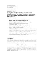
24 Fixed Point Theory and Applications
1009080706050403020100
Number of iterations
0
0.1
0.2
0.3
0.4
0.5
0.6
0.7
x
n
a 1
a 0.75
a 0.5
Figure 1
For x
1
0anda 1, the sequence {x
n
} defined by 6.1 can be explicitly written as
x
n
⎧
⎪
⎨
⎪
⎩
1
2
,n 2, 4, ;
n − 1
2n
,n 3, 5,
6.2
Observe that
1 T is nonexpansive,
2 F is both 1-strongly accretive and λ-strictly pseudocontractive over C for each λ>0,
3 RI − τF ⊆ C for each τ ∈ 0, 1,and
4 lim
n →∞
α
n
0,
∞
n1
α
n
∞ and lim
n →∞
|1 − α
n
/α
n1
| 0.
Thus, all the assumptions of Theorem 4.4 are satisfied. Therefore, the conclusion of
Theorem 4.4 holds, that is, x
n
→ 1/2 ∈ FT.
It is seen from Figure 1 that if a 1, a 0.75, and a 0.5, then the corresponding
iterations of sequence {x
n
} with x
1
0 defined by 6.1 are convergent to 1/2.
Example 6.2. Let H, C, T,andF be as in Example 6.1. Clearly T is nonexpansive and F is
both 1-strongly accretive and λ-strictly pseudocontractive over C for each λ>0. Assume that
{a
n
} is a sequence in 0, 1 such that
∞
n1
|a
n
− a
n1
| < ∞. Without loss of generality we may
assume that a
n
1/n
3/2
for all n ∈ N. For each n ∈ N, define T
n
: C → C by
T
n
x
⎧
⎨
⎩
1 − x, if x ∈
0, 1
,
a
n
, if x 1.
6.3
Define a sequence {α
n
} in 0, 1 by α
n
1/n for all n ∈ N.
Fixed Point Theory and Applications 25
We now show that, under the assumptions of Theorem 4.2, the sequence {x
n
}
generated by the proposed Algorithm 4.1 converges to a unique solution 1/2ofVIPF,C
over
n∈N
FT
n
. We proceed with the following steps.
Step 1. {T
n
} is a sequence of nearly nonexpansive mappings from C into itself such that
n∈N
FT
n
/
∅.
For x, y ∈ 0, 1, we have
T
n
x − T
n
y≤x − y∀n ∈ N. 6.4
Moreover, for x ∈ 0, 1 and y 1, we have
T
n
x − T
n
1 1 − x − a
n
≤x − 1 a
n
∀n ∈ N. 6.5
Thus,
T
n
x − T
n
y≤x − y a
n
∀x, y ∈ C, n ∈ N, 6.6
that is, {T
n
} is a sequence of nearly nonexpansive mappings from C into itself such that
n∈N
FT
n
{1/2}.
Step 2. lim
n →∞
T
n
z Tzfor all z ∈ C.
For each n ∈ N, we have
T
n
x − T
n1
x
⎧
⎨
⎩
0, if x ∈
0, 1
,
a
n
− a
n1
, if x 1,
6.7
and hence sup{T
n
x − T
n1
x : x ∈ C} |a
n
− a
n1
|. One can easily see that
∞
n1
D
C
T
n
,T
n1
∞
n1
sup
{
T
n
x − T
n1
x : x ∈ C
}
∞
n1
|
a
n
− a
n1
|
< ∞.
6.8
Since {T
n
} is a sequence of nearly nonexpansive self-mappings of C with sequence {a
n
}
such that
∞
n1
D
C
T
n
,T
n1
< ∞, it follows from Proposition 2.4 that for each x ∈ C, {T
n
x}
converges to some point of C. It can be readily seen that lim
n →∞
T
n
z Tzfor all z ∈ C.
Step 3. The sequence {x
n
} defined Algorithm 4.1 converges to 1/2 ∈ FT.