Advances in Measurement Systems Part 9 doc
Bạn đang xem bản rút gọn của tài liệu. Xem và tải ngay bản đầy đủ của tài liệu tại đây (1.74 MB, 40 trang )
AdvancesinMeasurementSystems316
The laser interferometers are mainly divided into two categories; homodyne and
heterodyne. The laser heterodyne interferometers have been widely used in displacement
measuring systems with sub-nanometer resolution. During the last few years
nanotechnology has been changed from a technology only applied in semiconductor
industry to the invention of new production with micro and nanometer size until in future
picometer size such as, nano electro mechanical systems (NEMS), semiconductor nano-
systems, nano-sensors, nano-electronics, nano-photonics and nano-magnetics (Schattenburg
& Smith, 2001).
In this chapter, we investigate some laser interferometers used in the nano-metrology
systems, including homodyne interferometer, two-longitudinal-mode laser heterodyne
interferometer, and three-longitudinal-mode laser heterodyne interferometer (TLMI).
Throughout the chapter, we use the notations described in Table 1.
2. Principles of the Laser Interferometers as Nano-metrology System
2.1 Interference Phenomenon
Everyone has seen interference phenomena in a wet road, soap bubble and like this. Boyle
and Hooke first described interference in the 17
th
century. It was the start point of optical
interferometry, although the development of optical interferometry was stop because the
theory of wave optics was not accepted.
A beam of light is an electromagnetic wave. If we have coherence lights, interference
phenomenon can be described by linearly polarized waves. The electrical field
E in
z
direction is represented by exponential function as (Hariharan, 2003):
cztiaE /2expRe
(1)
where
a is the amplitude, t is the time,
is the frequency of the light source and c is the
speed of propagation of the wave. If all equations on
E
are linearly assumed, it can be
renewed as:
(2)
tiia
ticziaE
2expexpRe
2exp/2expRe
The real part of this equation is:
iaA
tiAE
exp
2exp
(3)
where
nz
c
z
2
2
(4)
In this formula
is the wavelength of light and n is the refractive index of medium.
According to Fig. 1, if two monochromic waves with the same polarization propagate in the
same direction, the total electric field at the point P is given by:
(5)
21
EEE
Nano-metrologybasedontheLaserInterferometers 317
where
1
E and
2
E are the electric fields of two waves. If they have the same frequency, the
total intensity is then calculated as:
(6)
2
21
AAI
Constants & Symbols Abbreviations
amplitude of leakage electrical field
E
~
avalanche photodiode
APD
amplitude of main electrical field
E
ˆ
Band pass filter
BPF
secondary beat frequency
s
f
non-polarizing beam splitter
BS
higher intermode beat frequency
23
bH
f
corner cube prism
CCP
the lower intermode beat frequency
12
bL
f
double-balanced mixer
DBM
base photocurrent
b
I
frequency-path
FP
measurement photocurrent
m
I
I to V converter
IVC
refractive index of medium
n
low-coherence interferometry
LCI
target velocity
V
linear polarizer
LP
rotation angle of the PBS with respect
to the laser polarization axis
optical path difference
OPD
non-orthogonality of the polarized
beams
and
polarizing-beam splitter
PBS
ellipticity of the central and side
modes
rt
and
three-longitudinal-mode
interferometer
TLMI
Doppler shift
f
Vectors & Jones Matrices
the displacement measurement
z
matrix of LP
LP
the phase change
matrix of reference CCP
RCCP
the phase change resulting from
optical path difference
matrix of reference PBS
RPBS
the initial phase corresponding to the
electrical field of E
i
0
matrix of target CCP
TCCP
the wavelength of input source
matrix of target PBS
TPBS
the synthetic wavelength in two-mode
laser heterodyne interferometer
II
X
component of the total electric
field
X
LP
E
the synthetic wavelength in three-
mode laser heterodyne interferometer
III
Y
component of the total electric field
y
LP
E
the optical frequency
Constants & Symbols
the deviation angle of polarizer
referred to
45
the speed of light in vacuum
c
the reflection coefficients of the PBS
ellipticity of the polarized beams
d
optical angular frequency
electrical field vector
E
the transmission coefficients of the
PBS
the number of distinct interference
terms
the number of active FP elements
nonlinearity phase
Table 1. Nomenclatures
AdvancesinMeasurementSystems318
Fig. 1. Formation of interference in a parallel plate waves
(7)
cos2
2/1
2121
2121
2
2
2
1
IIII
AAAAAAI
where
1
I
and
2
I
are the intensities at point P, resulting from two waves reflected by surface
and
(8)
111
exp
iaA
(9)
222
exp
iaA
The phase difference between two waves at point P is given by:
(10)
zn
c
z
2
2
21
According to Eq. (10), the displacement can be calculated by detecting the phase from
interference signal. An instrument which is used to measure the displacement based on the
interferometry phenomenon is interferometer. Michelson has presented the basic principals
of optical displacement measurement based on interferometer in 1881. According to using a
stabilized He-Ne as input source (Yokoyama et al., 1994; Eom et al., 2002; Kim & Kim, 2002;
Huang et al., 2000; Yeom & Yoon, 2005), they are named laser interferometers. Two kinds of
laser interferometers depending on their detection principles, homodyne or heterodyne
methods, have been developed and improved for various applications.
Homodyne interferometers work due to counting the number of fringes. A fringe is a full
cycle of light intensity variation, going from light to dark to light. But the heterodyne
interferometers work based on frequency detecting method that the displacement is arrived
from the phase of the beat signal of the interfering two reflected beams. On the other hand,
heterodyne method such as Doppler-interferometry in comparison with homodyne method
provides more signal-to-noise ratio and easier alignment in the industrial field applications
(Brink et al., 1996). Furthermore, the heterodyne interferometers are known to be immune to
environmental effects. Two-frequency laser interferometers are being widely used as useful
instruments for nano-metrology systems.
Nano-metrologybasedontheLaserInterferometers 319
2.2 Homodyne Interferometer
Commercial homodyne laser interferometers mainly includes a stabilized single frequency
laser source, two corner cube prisms (CCPs), a non-polarizing beam splitter (BS), two
avalanche photodiodes (APDs), and measurement electronic circuits. The laser frequency
stabilization is many important to measure the displacement accurately. A laser source used
in the interferometers is typically a He-Ne laser.
An improved configuration of the single frequency Michelson interferometer with phase
quadrature fringe detection is outlined in Fig. 2. A 45º linearly polarized laser beam is split
by the beam splitter. One of the two beams, with linear polarization is reflected by a CCP
r
which is fixed on a moving stage. The other beam passes through a retarder twice, and
consequently, its polarization state is changed from linear to circular. The electronics
following photodetectors at the end of interferometer count the fringes of the interference
signal (see section 3.2). With interference of beams, two photocurrent signals
x
I
and
y
I
are
concluded as:
(11)
z
n
aI
y
4
sin
(12)
z
n
bI
x
4
cos
where
z
is the displacement of CCP
t
which is given by:
(13)
x
y
I
I
n
z
1
tan
4
This is called a DC interferometer, because there is no dependency to the time in the
measurement signal (Cosijns, 2004).
2.3 Heterodyne Interferometer
A heterodyne laser interferometer contains a light source of two- or three-longitudinal-mode
with orthogonal polarizations, typically a stabilized multi-longitudinal-mode He-Ne laser.
The basic setup of a two-mode heterodyne interferometer is shown in Fig. 3. The electric
field vectors of laser source are represented by:
(14)
1011011
2exp
ˆ
etEE
(15)
2022022
2exp
ˆ
etEE
where
01
ˆ
E
and
02
ˆ
E
are the electric field amplitudes,
1
and
2
are the optical frequencies
stabilized in the gain profile and
01
and
02
represent the initial phases. As it can be seen
from Fig. 3, the optical head consists of the base and measurement arms. The laser output
beam is separated by a non-polarizing beam splitter from which the base and measurement
beams are produced. The base beam passing through a linear polarizer is detected by a
AdvancesinMeasurementSystems320
photodetector. Consequently, in accordance with Eq. (6), the base photocurrent
b
I with
12
intermode beat frequency is obtained as:
(16)
0102120201
2cos
ˆˆ
2
tEEI
b
BS
y
I
x
I
Retarder
LP
CCP
r
CCP
t
Single Frequency
He-Ne Laser
PBS
Electronic
Section
Fig. 2. The schematic representation of homodyne laser interferometer
m
I
b
I
1
2
f
2
1
Fig. 3. The schematic representation of heterodyne laser interferometer
As it is concluded from Eq. (16), the heterodyne interferometer works with the frequency
(
12
), therefore it is called an AC interferometer. The measurement beam is split into two
beams namely target and reference beams by the polarizing-beam splitter (PBS) and are
directed to the corner cube prisms. The phases of modes are shifted in accordance with the
optical path difference (OPD). To enable interference, the beams are transmitted through a
linear polarizer (LP) under 45º with their polarization axes. After the polarizer, a
photodetector makes measurement signal
m
I :
(17)
rtm
tEEI
0102120201
2cos
ˆˆ
2
The phase difference between base and measurement arms represents the optical path
difference which is dependent to the displacement measurement. As the CCP
t
in the
measurement arm moves with velocity
V , a Doppler shift is generated for
2
:
Nano-metrologybasedontheLaserInterferometers 321
(18)
c
Vn
f
2
2
2
The phase change in the interference pattern is dependent on the Doppler frequency shift:
(19)
z
c
n
t
t
t
2
4
2
2
1
Finally, the displacement measurement of the target with vacuum wavelength
2
is given as:
(20)
n
z
4
2
3. Comparison Study between Two- and Three-Longitudinal-Mode Laser
Heterodyne Interferometers
3.1 The Optical Head
To reach higher resolution and accuracy in the nanometric displacement measurements, a
stabilized three-longitudinal-mode laser can replace two-longitudinal-mode laser. In the
two-mode interferometer, one intermode beat frequency is produced, whereas in three-
mode interferometer three primary beat frequencies and a secondary beat frequency appear.
Although the three-longitudinal-mode interferometers (TLMI) have a higher resolution
compared to two-longitudinal-mode type, the maximum measurable velocity is
dramatically reduced due to the beat frequency reduction. Yokoyama et al. designed a
three-longitudinal-mode interferometer with 0.044 nm resolution, assuming the phase
detection resolution of 0.1º (Yoloyama et al., 2001). However, limitation of the velocity in the
displacement measurement can be eliminated by a proper design (Yokoyama et al., 2005).
The source of the multiple-wavelength interferometer should produce an appropriate
emission spectrum including of several discrete and stabilized wavelengths. The optical
frequency differences determine the range of non-ambiguity of distance and the maximum
measureable velocity. The coherence length of the source limits the maximal absolute
distance, which can be measured by multiple-wavelength. If we consider a two-wavelength
interferometry using the optical wavelengths
1
and
2
with orthogonal polarization, the
phase shift of each wavelength will be:
(21)
i
z
i
4
where
z
is the optical path difference and
i
is the phase shift corresponding to the
wavelength
i
. Therefore, the phase difference between
1
and
2
is given by:
(22)
21
11
4
z
And the synthetic wavelength,
II
, can be expressed as:
AdvancesinMeasurementSystems322
(23)
2121
21
II
c
where
1
and
2
are the optical frequencies corresponding to
1
and
2
, and c is the
speed of light in vacuum. If the number of stabilized wavelengths in the gain curve increase
to three-longitudinal-mode, the synthetic wavelength is obtained as:
(24)
s
f
c
323121
321
II
2
where
s
f is the secondary beat frequency in the three-mode laser heterodyne
interferometers. Therefore, the synthetic wavelength in the three-longitudinal-mode
interferometer comparing to two-mode system is considerably increased (Olyaee & Nejad,
2007c). The stabilized modes in the gain profile of the laser source and optical head of the
nano-metrology system on the basis of two- and three-longitudinal-mode lasers are shown
in Fig. 4. As it is represented three wavelengths for which the polarization of the side modes
1
and
3
is orthogonal to the polarization of the central mode
2
. The electric field of
three modes of laser source is obtained as:
(25)
3,2,1,)2sin(
ˆ
itEE
iiii
where
i
is the initial phases corresponding to the electric field
i
E . In both cases, the
optical head consists of the base and measurement arms. First, the laser output is separated
by BS, so that base and measurement beams are produced. Then, the beam is split into two
subsequent beams by PBS and directed to each path of the interferometers. Two reflected
beams are interfered to each other on the linear polarizer. Because of orthogonally polarized
modes, the linear polarizer should be used to interfere two beams as shown in Fig. 5. The
stabilized multimode He-Ne lasers are chosen in which the side modes can be separated
from the center mode due to the orthogonal polarization states.
But in reality, non-orthogonal and elliptical polarizations of beams cause each path to
contain a fraction of the laser beam belonging to the other path. Hence, the cross-
polarization error is produced. In the reference path (path.1) of TLMI,
1
and
3
are the
main frequencies and
2
is the leakage one, whereas in the target path (path.2),
2
is the
main signal and the others are as the leakages.
Nano-metrologybasedontheLaserInterferometers 323
(a)
PBS
Path.2 (Target)
Measurement arm
BS
R
Base arm
Stabilized Two-Longitudinal-Mode
He-Ne Laser
21
,
b
f
1
2
2
1tor Photodetec
t
CCP
r
CCP
LP LP
21
,
2tor Photodetec
1
Two-Longitudinal-Mode Laser Heterodyne Interferometer
(b)
321
,,
H
b
f
L
b
f
1
2
3
321222
E
~
,E
~
,E
1tor Photodetec
t
CCP
r
CCP
321
,,
2tor Photodetec
213111
E
~
,E,E
Fig. 4. The stabilized modes in gain profile and optical head of the nano-metrology system
based on (a) the two- and (b) three-longitudinal-mode He-Ne laser interferometers
x
E
y
E
t
E
r
E
c
o
s
θ
E
t
s
i
n
θ
E
r
θ
Fig. 5. Combination of orthogonally polarized beams on the linear polarizer
AdvancesinMeasurementSystems324
(a)
Counter
COMP.m
A.b
BPF.m
IVC.b
A.m
BPF.b COMP.b
Output
APD.b
IVC.m
APD.m
(b)
Opto.b
+
-
OUT
BPF.m1
A.b
Base
CLK
Measurement
CLK
R
APD.b
Accurate Phase Detector
+
-
OUT
DBM.b
IVC.m A.m
Rc
BPF.b1
HI
1
2
3
4
Digital GND
Digital Section
Rf
APD.m
Comp.b
BPF.b2
HI
+ High Voltage.2
Analog GND (base)
R
1
2
3
4
BPF.m2
Comp.m
DBM.m
Measurement arm
IVC.b
Analog GND (measurement)
Microcontroller
+ High Voltage.1
High Speed Up/Down Counters
Rf
Rc
Opto.m
Base arm
Fig. 6. The schematic of the electronic circuits of the nano-metrology system based on the (a)
two- and (b) three-longitudinal-mode laser interferometers
Owing to the square-law behavior of the photodiodes, the reference signal is expressed as:
(26)
DtfCtfBtffA
DtCtBtAI
bLbHbLbH
APD
b
2cos2cos2cos
2cos2cos2cos
122313
Similarly, the output current of the measurement avalanche photodiode, APD
m
, is:
(27)
DtffCtffBtffAI
bLbHbLbHAPD
m
2cos2cos2cos
where
A
,
B
, C , and D are constant values and f is the frequency shift due to the
Doppler effect and its sign is dependent on the moving direction of the target. To extract the
phase shift from Eqs. (26) and (27), two signals are fed to the proper electronic section as
described in the following.
Nano-metrologybasedontheLaserInterferometers 325
3.2 The Electronic Sections
The schematic diagram of the electronic circuits of the two- and three-longitudinal-mode
laser interferometers are shown in Fig. 6. In both systems, the photocurrents of the
avalanche photodiodes are amplified and converted to voltage signals. In two-mode system,
the amplified signals pass through the band-pass filters (BPFs) involving the intermode beat
frequency (typically several hundred MHz which can be reduced by heterodyne technique).
Parameter Two-Longitudinal-
Mode Laser
Interferometer
Three-Longitudinal-
Mode Laser
Interferometer
Unit
Wavelength 632.8 632.8 nm
Cavity length 25 35 cm
Synthetic wavelength 0.5 1000 m
Maximum absolute distance 0.25 500 m
Intermode beat frequency
600 435.00, 435.30, 870.30
MH
z
Secondary beat frequency 300 kHz
Maximum measurable velocity 21 0.047 m/s
Phase detection accuracy (similar
circuit)
11.8 5.9 pm
Cross-talk and intermodulation
distortion error
100 18 pm
The number of active frequency-path
elements
4 6
The number of
distinct interference
terms
Optical power
Total: 10
4
Total: 21
6
AC
interference
2 6
DC
interference
2 3
AC reference
2 6
Table 2. A comparison between two- and three-longitudinal-mode He-Ne laser
interferometers with typical values (Olyaee & Nejad, 2007c)
Two signals from base and measurement arms are then fed to a counter to measure the
target displacement resulting from optical path difference.
But in TLMI, the amplified signals are self-multiplied by two double-balanced mixers, DBM
b
and DBM
m
. As a result, the secondary beat frequency generates (typically several hundred
kHz). The high frequency and DC components are eliminated by two band-pass filters,
BPF
b2
and BPF
m2
. The input signals of the comparators for base and measurement arms are
respectively described as:
(28)
tfkV
sob
2cos'
(29)
22cos' tfkV
som
The phase shift resulting from optical path difference is measured by a high-speed
up/down counter. The base and measurement signals can be exerted to a half exclusive-or
gate and the pulse width is measured by a high speed counter. The phase difference
between the base and measurement signals is proportional to the output pulse width. The
AdvancesinMeasurementSystems326
resolution of the phase detector is proportional to the clock pulse of the counter. The phase
shift due to optical path difference is given by:
(30)
z
n
2
4
where
2
is the central wavelength. It should be noted that in Eq. (29), the phase shift is
multiplied by 2 which indicates the resolution in TLMI is doubled compared to two-mode
type (see Eq. (17)).
On the other hand, the maximum measurable velocity corresponding to Eq. (18) is
dependent on the intermode beat frequencies. In the TLMI, because we use super-
heterodyne method to extract the secondary beat frequency (that is much smaller than
primary beat frequencies produced in the TLMI or than intermode beat frequency in two-
mode type), the maximum measurable velocity to be considerably reduced.
A comparison between two- and three-mode laser interferometers with typical values is
summarized in Table 2. The maximum measurable velocity for two-mode type is about
21m/s, whereas in TLMI it is limited to 47.46mm/s. But according to Table 2, the resolution
of the displacement measurement and synthetic wavelength in the three-longitudinal-mode
is considerably increased. The output signals of the measurement double-balanced mixer
and band-pass filter for fixed target, -47 mm/s, -20 mm/s, and +47 mm/s target velocities
are shown in Fig. 7.
3.3 The Frequency-Path Modeling
A multi-path, multi-mode laser heterodyne interferometer can be described by a frequency-
path (FP) model. The frequency-path models of two- and three-longitudinal-mode
interferometers are shown in Fig. 8. In the measurement arm of TLMI, there are three
frequency components and two paths namely the reference and the target (the bold lines are
the main signal paths and the dashed lines are the leakage paths), whereas in two-
longitudinal-mode interferometer, there are two frequency components and two paths. The
number of active frequency-path elements,
, is obtained by multiplying the number of
frequency components by paths (Schmitz & Beckwith, 2003). Consequently, in two-path,
two- and three-mode interferometers, the number of active FP elements is 4 and 6,
respectively.
Figure 9 shows the identification of the physical origin of each frequency-path element for
the measurement arms of two- and three-mode interferometers. Because the wave intensity
being received by an APD is proportional to the square of the total electrical field, the
number of distinct interference terms is equal to:
(31)
21
2
1
In TLMI, the reference path field can be described by:
(32)
321)(cos
1
11
,,i,zktωEE
iiiii
Nano-metrologybasedontheLaserInterferometers 327
0 2 4 6
-1 0
-5
0
5
10
Amp li tu de (V)
V = - 4 7 m m/s e c
0 2 4 6
-10
-5
0
5
10
V = - 2 0 m m/s e c
0 2 4 6
-5
0
5
10
Amp l itu de (V)
Ti m e (u s )
V = 0 m m /s e c
0 2 4 6
-5
0
5
10
Ti m e (u s )
V = + 4 7 m m/s e c
D B M o u tp u t
LP F o utp u t
Fig. 7. The output signals of the measurement BPF and DBM (Olyaee & Nejad, 2007b)
m
APD
b
APD
1
2
m
APD
b
APD
1
2
3
Fig. 8. The frequency-path model in two- and three-longitudinal-mode laser interferometers
where
ij
is the initial phases corresponding to the electrical field
ij
E
,
i
k
is the propagation
constant or wave number
i
/2
,
ii
2
is the optical angular frequency, and
1
z
is
the motion of the corner cube prism in the reference path (CCP
r
). Similar to Eq. (32), the
target path field is described by:
(33)
321)(cos
2
22
,,i,zktωEE
iiiii
where
2
z
is the motion of the corner cube prism in the target path (CCP
t
). In this system, the
CCP
r
is fixed and hence,
0
1
z
. Furthermore, the wavelengths are so close that propagation
constants become almost equal to each other (
kkkk
321
). The high frequency
components such as
i
,
i
2
and
j
i
are eliminated by the avalanche photodiodes
(
321, ,,ji
). Therefore, ignoring the high frequencies in the fully unwanted leaking
interferometers, there are 21 distinct interference terms for three-longitudinal-mode
AdvancesinMeasurementSystems328
interferometer and 10 distinct interference terms for two-mode type (see Table 2). The
distinct interference terms can be divided into four groups namely dc interference (DI), ac
interference (AI), ac reference (AR), and optical power (OP). These components in the three-
longitudinal-mode interferometer are respectively given by (Olyaee & Nejad, 2007a):
(34)
)(cos
~
)(cos
~
)(cos
~
232312222121211
kzEEkzEEkzEE/KI
DI
(35)
)(cos))((cos
~
)(cos
~~
)(cos
~~
))((cos
~
)(cos
222312123123221
212212321122211
kztωEEkztωωEEkzωEE
kztωEEkztωωEEkztωEE/KI
bHbLbHbH
bLbLbHbLAI
(36)
))cos((
~~
)cos(
~~
)cos(
~~
31113212
3222312122122111
tωωEEEE
tωEEEEtωEEEE/KI
bLbH
bHbLAR
(37)
2
32
2
22
2
12
2
31
2
21
2
11
~~~
2
1
EEEEEE/KI
OP
Figure 10 shows the combination of the frequency-path elements in the measurement arm of
two systems. The main signals and leakages are depicted by large and small solid circles,
respectively. On the other hand, the diameter of the circles presents the amplitude of the
signals. The small solid circles are exaggerated for clarification. All of the distinct
interference terms are shown in Fig. 10 by different lines.
(a)
11
E
21
E
~
12
E
~
22
E
1
1
2
2
Nano-metrologybasedontheLaserInterferometers 329
(b)
11
E
13
E
12
E
~
1
1
3
21
E
~
23
E
~
3
2
22
E
2
Fig. 9. Identification of the physical origin of each frequency-path element in the reference
and target paths (measurement arms). (a) Two- and (b) Three-longitudinal-mode laser
interferometers
22
E
11
E
31
E
12
E
~
32
E
~
21
E
~
11
E
12
E
~
21
E
~
22
E
(a) (b)
Fig. 10. The combination graph of the frequency-path elements in (a) two- and (b) three-
longitudinal-mode interferometers
AdvancesinMeasurementSystems330
4. Nonlinearity Analysis
In section 2, we have shown that for a heterodyne interferometer the displacement could be
determined by measuring the phase change between measurement and base signals. From
Eq. (20), it can be seen that the accuracy of the displacement depends on the accuracy of the
determination of the phase change, the wavelength of light and the refractive index of the
medium. But, the displacement accuracy is also influenced far more by setup configuration,
instrumentation section and environmental effects (Cosijns, 2004).
The first group is related to misalignment and deviations in the optical setup and
components such as polarizer, polarizing-beam splitter and laser head. These can be
minimized or even eliminated by using a correct setup and alignment procedures. In the
second group related to electronic and instrumentation section includes laser frequency
instability, phase detection error and data age uncertainty (Demarest, 1998). Instability in
the mechanical instruments, cosine error and Abbe error are directly related to the setup
configuration. The accuracy of refractive index determination, turbulences and thermal
instability are the environmental parameters affecting the accuracy of the displacement
(Bonsch & Potulski 1998;
Wu, 2003; Edlen, 1966). In the mentioned errors, several of them
are considered as linear errors that can be simply reduced or compensated.
When the measured displacement with a non-ideal interferometer is plotted against the real
displacement of the moving target an oscillation around the ideal straight line is observed.
This effect is known as a periodic deviation of the laser interferometer (Cosijns, 2004). The
stability of the laser source, alignment error, vibration, temperature variation and air
turbulence are the main sources of error for the optical interferometer. If all of the above
conditions can be kept good enough, then the practical limitations will be given by the
photonic noise and the periodic nonlinearity inherent in the interferometer (Wu & Su, 1996).
The nonlinearity of one-frequency interferometry is a two-cycle phase error, whereas in
heterodyne interferometry is mainly a one-cycle phase error as the optical path difference
changes from 0 to 2π. Although the heterodyne interferometers have a larger nonlinearity than
do the one-frequency interferometers, with first-order versus second-order error, the first-
order nonlinearity of heterodyne interferometers can be compensated on-line (Wu et al, 1996).
In the ideal heterodyne interferometers, two beams are completely separated from each other
and traverse with pure form in the two arms of the interferometer. Although the heterodyne
method compared to the homodyne method provides more signal to noise ratio and easy
alignment, in contrast, because of using two separated beams in the heterodyne method, the
nonlinearity errors especially cross-talk and cross-polarization dominate. The polarization-
mixing happens within an imperfect polarizing-beam splitter. This is nonlinearity error which
is often in the one frequency interferometer. Meanwhile in case of heterodyne laser
interferometer, frequency mixing error which arises from non-orthogonality of the polarizing
radiations, elliptical polarization and imperfect alignment of the laser head and other
components produce periodic nonlinearity error (Cosijns et al., 2002; Freitas, 1997; Eom et al.
2001; Hou & Wilkening 1992; Meyers et al., 2001; Sutton, 1998). The two waves, which are
regarded as orthogonal to each other in a heterodyne interferometer, are not perfectly
separated by the polarizing-beam splitter, with the result that the two frequencies are mixed.
The mixing leads to a nonlinear relationship between the measured phase and the actual
phase, and limits the accuracy of the heterodyne interferometer with a two-frequency laser to a
few nanometers. The periodic nonlinearity can be analytically modeled by both Jones calculus
and plane wave which will be described in the next two sections.
Nano-metrologybasedontheLaserInterferometers 331
4.1 Analytical Modeling of the Periodic Nonlinearity based Jones Calculus
According to the setup of TLMI in Fig. 4b, in both paths of the reference (reflected) and
target paths (transmitted), there are small fractions of oppositely polarized beams as a
leakage caused by the ellipticity of the laser mode polarization and misalignment of the
polarization axes between the laser beam and PBS. The leakage beams result in the
frequency mixing and produce the periodic nonlinearity in the detected heterodyne signal.
To have a model of nonlinearity in the TLMI, we first assume that the beam emerged from
the laser is to be elliptically polarized. The ellipticity of the central and side modes are
denoted by
t
and
r
, respectively, as usual. Then, the electric fields of three longitudinal
modes are respectively given as:
(38)
1
011
exp
sin
cos
ti
i
r
r
E
(39)
2
022
exp
cos
sin
ti
i
t
t
E
(40)
3
033
exp
sin
cos
ti
i
r
r
E
If the rotation angle of the PBS with respect to the laser polarization axis is denoted by
,
the matrix representing the PBS for reference and target beam directions respectively can be
calculated as :
(41)
cossin
sincos
00
01
cossin
sincos
RPBS
(42)
cossin
sincos
10
00
cossin
sincos
TPBS
3
2
1
E
E
E
2
2
sincossin
cossincos
10
01
2
2
sincossin
cossincos
2
2
coscossin
cossinsin
i
i
e
e
0
0
2
2
coscossin
cossinsin
2sin12cos
2cos2sin1
LPLP
EE
SKH
SHV
i
2
22cos tfgV
So
m
Fig. 11. Jones matrix components of the measurement arm of the TLMI with leakage fields.
The dashed lines indicate optical leakage
AdvancesinMeasurementSystems332
The Jones matrix for linear polarizer oriented at
o
45 relative to the polarization directions is
then described by:
(43)
)45(sin)45sin()45cos(
)45sin()45cos()45(cos
2
2
LP
Figure 11 shows the simplified matrices for optical components of the target and reference
paths including the optical leakages in the TLMI. The optical leakages are shown by dashed
lines (Olyaee et al., 2009).
According to Fig. 11, the Jones vector of the reference electrical field incident upon the linear
polarizer is obtained as:
(44)
3
1
l
l
ERPBSRCCPRPBSE
r
where
RCCP
is the Jones matrix for reference corner cube prism (CCP
r
) in the reference
path which is given by:
(45)
10
01
RCCP
If the reflection coefficient of the PBS in the reference path direction is denoted as
, by
substitution of the related Jones matrices, Eq. (44) can be rewritten as:
(46)
2
31
02
0301
22
22
exp
expexp
cossinsincossinsinsincoscossin
coscossinsincossincossincoscos
ti
titi
ii
ii
ttrr
ttrr
r
E
Similar to Eq. (44), the target electrical field is given by:
(47)
2
31
02
0301
22
22
3
1
exp
expexp
coscossincossinsincoscoscossin
coscossinsinsinsincossincossin
ti
titi
ii
ii
ttrr
ttrr
l
l
ETPBSTPBS.TCCP.E
t
where
is the transmission coefficient of the PBS in the target path direction and
TCCP
is
the Jones matrix for corner cube prism in the target path which is given by:
(48)
i
i
exp0
0exp
TCCP
Nano-metrologybasedontheLaserInterferometers 333
The reflected beam of the reference path and the transmitted beam from the target path at
the output port of the PBS interfere with each other through the linear polarizer. Therefore,
the final electric field vector after passing through the linear polarizer (LP) is obtained by:
(49)
rtLP
EELPE
The intensity of the laser beam which is proportional of the photocurrent at the detector can
be obtained by pre-multiplying the Jones vector with its complex conjugate of the matrix
transpose. Consequently, the photocurrent detected by an avalanche photodiode can be
given as:
(50)
YYXXm
APD
I
LPLPLPLP
EEEE
**
where
X
LP
E
and
Y
LP
E
are the
X
and
Y
components of the total electric field vector,
respectively. By expanding Eq. (50) and eliminating the optical frequencies and dc
component, the Fourier spectrum components and phase terms of the time-dependent
photocurrent is obtained as:
(51)
titititi
titititi
titititi
APD
bHbLbHbL
bHbLbHbL
bHbLbHbL
m
eeicbeeicd
eeicdeeicb
eeiaeeeiaeI
where
(52)
****
YYYYXXXX
DCBADCBAiae
****
YYYYXXXX
CDABCDABiae
**
YYXX
DADAicb
**
YYXX
CBCBicd
**
YYXX
BCBCicd
**
YYXX
ADADicb
and
(53)
rr
rr
i
iA
X
sinsincoscossin2cos
sincossincoscos12sin/
2
2
(54)
tt
tt
i
iB
X
cossinsincossin2cos
coscossinsincos2sin1/
2
2
(55)
rr
rr
i
iC
X
sincoscoscossin2cos
sincossincossin2sin1/
2
2
(56)
tt
tt
i
iD
X
coscossincossin2cos
coscossinsinsin2sin1/
2
2
(57)
rr
rr
i
iA
Y
sinsincoscossin2sin1
sincossincoscos2cos/
2
2
AdvancesinMeasurementSystems334
(58)
tt
tt
i
iB
Y
cossinsincossin2sin1
coscossinsincos2cos/
2
2
(59)
rr
rr
i
iC
Y
sincoscoscossin2sin1
sincossincossin2cos/
2
2
(60)
tt
tt
i
iD
Y
coscossincossin2sin1
coscossinsinsin2cos/
2
2
Finally, Eq. (51) can be simplified as:
(61)
ttettd
ttttc
ttbttaI
bHbLbHbL
bHbLbHbL
bLbHbHbLAPD
m
coscoscoscos
sinsinsinsin
coscossinsin
As shown in Fig. 6b, the photocurrent of the APD is further processed for the super-
heterodyning by using a double-balanced mixer (DBM) and band-pass filter (BPF). Because
of using the BPF, the higher frequency component and the dc component of the
photocurrent can be effectively filtered out, resulting in the detection of a heterodyne signal
oscillating only at the secondary beat frequency with a high signal-to-noise ratio. Thus, the
output voltage is proportional to:
(62)
' 2 2 2
2 2 2 2
2 2 cos 2 sin
2 cos 2 sin 2 sin
2 cos 2 sin 2 2 sin 2
cos 2 cos 2
m
o S S
S S S
S S S
S S
V a bd c e t ab ce t
ac be t cb cd ae t ad ce t
ac de t bc t cd t
b c t d c t
To extract the phase nonlinearity from the above analytical formula, Eq. (62) could be
simplified as:
(63)
D
N
tNDtNtDV
SSSm
122
tan2cos2sin2cos
where
(64)
,4cos4sin23cos2
3sin22sin2cos2
sin22cos22
2222
222
cdcbcddeac
ceadaecdcbbeac
ceabecbdaD
(65)
,4sin4cos223sin2
3cos22cos2sin2
cos22sin22
22
222
cdcdbcdeac
ceadaecdcbbeac
ceabecbdaN
And the phase nonlinearity can be finally calculated as:
(66)
D
N
1
tan
This nonlinearity causes to appear the periodic nonlinearity in the displacement
measurement.
Nano-metrologybasedontheLaserInterferometers 335
4.2 Analytical Modeling of the Periodic Nonlinearity based Plane Waves
Another method for nonlinearity modeling is based on the plane wave method. By using
these approaches, a similar model for periodic nonlinearity is obtained. Here, the electrical
field vectors of side modes,
3,1
E
, and central mode,
2
E
, emerging from the three-
longitudinal-mode laser source with ellipticity of the reference and target beams are
respectively given as:
(67)
)2cos(sin))2sin()2sin(cos
02202033011013,1
tEttE
rr
E
(68)
)2sin(cos))2cos()2(cos(sin
02202033011012
tEttE
tt
E
Considering the non-orthogonality of the polarized beams in combination with the
deviation angle of PBS with respect to the laser head,
and
, a leakage of modes
appears. The electrical field magnitudes of the transmitted and reflected beams by the PBS
are given by:
(69)
)()(
cos
sin
213 titit
xExE
E
(70)
)()(
cos
sin
213 ririr
xExE
E
Here the terms
ii
t
0
2
denoted by
i
x
,
3,2,1i
and
and
are the transmission and
reflection coefficients of the PBS and
t
and
r
are the optical phase shift in the target and
reference paths, respectively. If the deviation angle of polarizer referred to
45
is
represented as
, the output of measurement photocurrent is corrected as:
(71)
2
)45sin()45cos(
trAPD
EEI
m
With detection of secondary beat frequency by the super-heterodyne detection, the
nonlinearity phase error is concluded similar to Eq. 66:
(72)
2cos2sin2cos2sincos
sincossincossin
109876
54321
sssss
sssssm
xCxCxCxCxC
xCxCxCxCxCV
where
(73)
2131211
2 BBBBAAC
32
2
1
2
2
2
12
22 BBBAAC
12213
2 BABAC
22114
2 BABAC
12315
2 BABAC
32116
2 BABAC
AdvancesinMeasurementSystems336
217
2 BBC
2
2
2
18
BBC
319
2 BBC
2
3
2
110
BBC
and
(74)
)cossin(sincos)sincos(cossin
2
1
2
2
2
1
2
21
KKKKA
trtr
)cos()sincoscossin(
212
rt
KKA
)cossincossinsincossincos(
31
trtr
KB
)coscoscoscossinsinsin(sin
32
trtr
KB
)coscossinsinsinsincos(cos
33
trtr
KB
)45(cos
2
00
2
1
23,1
EEK
)45(sin
2
00
2
2
23,1
EEK
)45cos()45sin(
23,1
003
EEK
Here the nonlinearity is given by Eq. (66) and following equations:
(75)
)4sin()4cos()3sin()3cos()sin(
)cos()2sin()2cos(
1097654
321
CCCCCC
CCCN
(76)
)4cos()4sin()3cos()3sin(
)cos()sin()2cos()2sin(
109865
4321
CCCCC
CCCCD
4.3 Error Analysis in the TLMI
Deviation angle and unequal transmission- reflection coefficients of the PBS
Considering the orthogonal linearly polarized modes, the effect of the PBS deviation angle is
described by
. The periodic nonlinearities in terms of the nanometric displacement in
the TLMI and two-mode interferometer are respectively illustrated in Fig. 12a and 12b. The
range of displacement is equal to the one wavelength of the He–Ne laser at 632.8 nm. The
result appears as the second-order nonlinearity. If the transmission and reflection
coefficients of the PBS are equal, then the periodic nonlinearity does not change. The
unequal coefficients and the mismatch between the factors causes the first-order
nonlinearity dominates, as shown in Fig. 12c (curve 3).
Non-orthogonality associated with deviation angle of the PBS
If there is non-orthogonality even in the absence of deviation angle, there will be a leakage
of modes. The effect of non-orthogonality of the polarized modes in combination with the
deviation angle of PBS is represented by
and is shown in Fig. 12d. Unlike Fig. 12a,
the periodic nonlinearity due to the non-orthogonality of polarized modes is represented as
the first order nonlinearity (see curve 1 in Fig. 12d for orthogonality).
Nano-metrologybasedontheLaserInterferometers 337
Non-orthogonality in combination with ellipticity of adjacent polarized modes
Considering the TLMI free of nonlinearity except for one-ellipticity of the polarizations
0
t
, and two-elliptical polarized modes, the periodic nonlinearity is the first-order type
of nonlinearity. But, if ellipticity of the polarized modes occurs simultaneously with
orthogonality, it may reproduce the second-order nonlinearity (see curves 2 and 3 in Fig.
12e). The nonlinearity generated in the displacement measurement in one fourth of the laser
wavelength range (158.2 nm) resulting from the ellipticity of laser polarization states for
ideal alignment (
0
deg) and non-ideal alignment (
3
deg) are compared in Fig. 13. The
nonlinearity error increases with increasing misalignment.
Rotation angle of the polarizer
A small rotation angle of the polarizer can provide nonlinearity, it can be appropriately
utilized for nonlinearity compensation in a proper optical setup. The nonlinearity resulting
from the two-ellipticity of the adjacent orthogonal and non-orthogonal polarized modes
associated with the rotation angle of the polarizer is shown in Fig. 12f.
-4 0 0 -2 0 0 0 2 0 0 40 0
-0 .1
-0 .05
0
0.0 5
0.1
Pe ri o d ic n on l i n ea r ity , n m
Di s pl a ce m en t, nm
-4 0 0 -2 0 0 0 2 0 0 40 0
-0 .1
-0 .05
0
0.0 5
0.1
D is pl a ce m en t, n m
Pe ri o d ic n on l i n ea r ity , n m
-4 0 0 -2 0 0 0 2 0 0 40 0
-0 .2
-0 .1
0
0.1
0.2
0.3
Pe ri o d ic n onl i n ea r ity , nm
Di s pl a ce m en t, nm
-4 0 0 -2 0 0 0 2 0 0 40 0
-3
-2
-1
0
1
2
3
D is pl a ce m en t, n m
Pe ri o d ic n on l i ne a ri ty , n m
-4 0 0 -2 0 0 0 2 0 0 40 0
-3
-2
-1
0
1
2
3
Di s pl a ce m en t, nm
Pe ri o d ic n on l i ne a ri ty , n m
-4 0 0 -2 0 0 0 2 0 0 40 0
-5
0
5
D is pl a ce m en t, n m
Pe ri o d ic n on l i n ea r ity , n m
(a ) (b )
(c)
(d )
(e ) (f)
Fig. 12. Periodic nonlinearity resulting from various optical deviations. The orthogonal
linearly polarized modes in the (a) three-mode interferometer and (b) two-mode
interferometer. (c) Orthogonal linearly polarized modes in combination with unequal
transmission and reflection coefficients. (d) The orthogonal (curve 1) and non-orthogonal
(curves 2 and 3) linearly polarized modes in combination with deviation angle of PBS. (e)
One-ellipticity of the adjacent orthogonal polarized modes. (f) Two-ellipticity of the adjacent
orthogonal (curve 2) and non-orthogonal (curves 1 and 3) polarized modes in combination
with the rotation angle of polarizer
Curve 1
Curve
2
Curve
3
AdvancesinMeasurementSystems338
-100
0
100
200
-0.4
-0.2
0
0.2
0.4
-6
-4
-2
0
2
4
6
Displacement of Target CCP (nm)Ellipticity (degree)
Displacement Error (nm)
-100
0
100
200
-0.4
-0.2
0
0.2
0.4
-6
-4
-2
0
2
4
6
Displacement of Target CCP (nm)Ellipticity (degree)
Displacement Error (nm)
(a) (b)
Fig. 13. The error of displacement measurement resulting from ellipticity of laser
polarization states for (a) ideal alignment (
o
0
) and (b) non-ideal alignment (
o
3
)
3
2
1
E
E
E
i
t
exp
coscossin
cossinsin
2
2
2
2
sincossin
cossincos
r
2sin12cos
2cos2sin1
2sin12cos
2cos2sin1
LPLP
EE
SKH
SHV
i
2
LPLP
EE
SKH
SHV
i
2
Fig. 14. The block diagram of nonlinearity reduction system
4.4 Nonlinearity Reduction
To reduce the nonlinearity in two-mode heterodyne interferometers, various kinds of
heterodyning systems and methods are still being developed (Wuy & Su, 1996; Freitas, 1997;
Wu, 2003; Badami & Patterson, 2000; Lin et al., 2000; Hou, 2006; Hou, & Zhaox, 1994). A
basic block diagram of the optical and electrical nonlinearity reduction system designed for
TLMI is schematically represented in Fig. 14. Two linear polarizers oriented at
45 and
45 , two avalanche photodiodes and a half-wave plate is used in the measurement arm.
The current-to-voltage converter, pre-amplifier and band-pass filter is denoted by transfer
function KH(S).
The output voltage is led to the double-balanced mixer and other band-pass filter to extract
the secondary beat frequency. The electrical cross-talk error occurs due to the unwanted
Nano-metrologybasedontheLaserInterferometers 339
induction between the electrical section of the base and measurement arms. This error can
be reduced by: (i) coupling reduction between the base and measurement arms using a
proper shielding, grounding and utilizing two isolated power supplies, (ii) noise reduction
by using electromagnetic interference shield, (iii) electrical power reduction and (iv)
utilizing the band pass filters with high quality factors.
A schematic diagram of the nano-displacement measurement based on the TLMI with noise
and electrical error reduction is shown in Fig. 15. The unwanted electrical induction
between the base and measurement paths is reduced by using two isolated power supplies
for APD biasing and by separating the grounds (analogue-base, analogue-measurement and
digital grounds). Due to switching noise of digital section including frequency and phase
measurement circuits and microcontroller, two high-speed opto-couplers isolate the
analogue circuits from digital section.
In order to reduce the periodic nonlinearity, two output signals can be averaged as shown in
Fig. 14. Therefore noise and electrical cross-talk are considerably reduced.
The corresponding compensated nonlinearity signals are depicted in the right panels
parallel to the left panels of Fig. 16. The four-cycle peak-to-peak periodic nonlinearity can be
effectively reduced from 38 pm to 1.2 pm, as shown in Fig. 16d. But 124 pm eight-cycle
nonlinearity cannot be reduced (see Fig. 16c).
BPF Comp.m
m1
APD
.
m2
b1
DBM
Base APD Biasing
APD
b
m3
DBM
Measurement APDs Biasing
b2
5
0
.
Rf
DBM
b1
m1
Isolated Power
Supply
R2
b2
BPF
A
A
BPF
m4
R3
.
+
-
OUT
1
2
3
4
A
Base Clock Pulse
.
BPF
R1
m2
Averaging
Circuit
A
Measurement Clock Pulse
Rc
A
+
-
OUT
b
Digital GND
Rc High Speed Up/Down Counter
& Accurate Phase Detector
b
+
-
OUT
m2
m1
Analog GND (base)
Rc
Iso.b
.
A
1
2
3
4
m4
IVC
Analog GND (measurement)
Rc
m2
m3
.
IVC
Rf
m1
BPF
Iso.m
IVC
m2
Rf
APD
BPF
Comp.b
+
-
OUT
m1
5
0
Fig. 15. The designed TLMI with noise, nonlinearity and error reduction