Advances in Robot Manipulators Part 3 pptx

AdvancesinRobotManipulators72


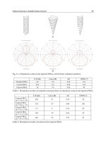
Fig. 23. Manipulability index - Wd = [1, 1, 1, 1, 1, 1, 1, 100, 100].

In all three cases, the manipulability measure was maximized based on the weight matrix.
Figure 21 shows an improvement trend of the WMRA’s manipulability index over the arm’s
manipulability index towards the end of simulation. Figure 22 shows the manipulability of
the arm as nearly constant compared to that in Figure 23 because of the minimal motion of
the arm. Figure 23 shows how the wheelchair started moving rapidly later in the simulation
(see figure 20) as the arm approached singularity, even though the weight of the wheelchair
motion was heavy. This helped in improving the WMRA system’s manipulability.

6.2 Simulation Results in an Extreme Case
To test the difference in the system response when using different methods, an extreme case
was tested, where the WMRA system is commanded to reach a point that is physically
unreachable. The end-effector was commanded to move horizontally and vertically
upwards to a height of 1.3 meters from the ground, which is physically unreachable, and the
WMRA system will reach singularity. The response of the system can avoid that singularity
depending on the method used. Singularity, joint limits and preferred joint-space weights
were the three factors we focused on in this part of the simulation. Eight control cases
simulated were as follows:
(a) Case I: Pseudo inverse solution (PI): In this case, the system was unstable, the joints
went out of bounds, and the user had no weight assignment choice.
(b) Case II: Pseudo inverse solution with the gradient projection term for joint limit
avoidance (PI-JL): In this case, the system was unstable, the joints stayed in bounds, and
the user had no weight assignment choice.
(c) Case III: Weighted Pseudo inverse solution (WPI): In this case, the system was unstable,
the joints went out of bounds, and the user had weight assignment choices.

(d) Case IV: Weighted Pseudo inverse solution with joint limit avoidance (WPI-JL): In this
case, the system was unstable, the joints stayed in bounds, and the user had weight
assignment choices.
(e) Case V: S-R inverse solution (SRI): In this case, the system was stable, the joints went
out of bounds, and the user had no weight assignment choice.
(f) Case VI: S-R inverse solution with the gradient projection term for joint limit avoidance
(SRI-JL): In this case, the system was unstable, the joints stayed in bounds, and the user
had no weight assignment choice.
(g) Case VII: Weighted S-R inverse solution (WSRI): In this case, the system was stable, the
joints went out of bounds, and the user had weight assignment choices.
(h) Case VIII: Weighted S-R inverse solution with joint limit avoidance (WSRI-JL): In this
case, the system was stable, the joints stayed in bounds, and the user had weight
assignment choices.
In the first case, Pseudo inverse was used in the inverse Kinematics without integrating the
weight matrix or the gradient projection term for joint limit avoidance. Figure 24 shows how
this conventional method led to the singularity of both the arm and the WMRA system. The
user’s preference of weight was not addressed, and the joint limits were discarded. In the
last case, the developed method that uses weighted S-R inverse and integrates the gradient
projection term for joint limit avoidance was used in the inverse kinematics. Figure 25 shows
the best performance of all tested methods since it fulfilled all the important control
requirements. This last method avoided singularities while keeping the joint limits within
bounds and satisfying the user-specified weights as much as possible. The desired trajectory
was followed until the arm reached its maximum reach perpendicular to the ground. Then it
started pointing towards the current desired trajectory point, which minimizes the position
errors. Note that the arm reaches the minimum allowed manipulability index, but when
combined with the wheelchair, that index stays farther from singularity.


Fig. 24. Manipulability index – using only Pseudo inverse in an extreme case.

A9-DoFWheelchair-MountedRoboticArmSystem:
Design,Control,Brain-ComputerInterfacing,andTesting 73


Fig. 23. Manipulability index - Wd = [1, 1, 1, 1, 1, 1, 1, 100, 100].

In all three cases, the manipulability measure was maximized based on the weight matrix.
Figure 21 shows an improvement trend of the WMRA’s manipulability index over the arm’s
manipulability index towards the end of simulation. Figure 22 shows the manipulability of
the arm as nearly constant compared to that in Figure 23 because of the minimal motion of
the arm. Figure 23 shows how the wheelchair started moving rapidly later in the simulation
(see figure 20) as the arm approached singularity, even though the weight of the wheelchair
motion was heavy. This helped in improving the WMRA system’s manipulability.

6.2 Simulation Results in an Extreme Case
To test the difference in the system response when using different methods, an extreme case
was tested, where the WMRA system is commanded to reach a point that is physically
unreachable. The end-effector was commanded to move horizontally and vertically
upwards to a height of 1.3 meters from the ground, which is physically unreachable, and the
WMRA system will reach singularity. The response of the system can avoid that singularity
depending on the method used. Singularity, joint limits and preferred joint-space weights
were the three factors we focused on in this part of the simulation. Eight control cases
simulated were as follows:
(a) Case I: Pseudo inverse solution (PI): In this case, the system was unstable, the joints
went out of bounds, and the user had no weight assignment choice.
(b) Case II: Pseudo inverse solution with the gradient projection term for joint limit
avoidance (PI-JL): In this case, the system was unstable, the joints stayed in bounds, and
the user had no weight assignment choice.
(c) Case III: Weighted Pseudo inverse solution (WPI): In this case, the system was unstable,
the joints went out of bounds, and the user had weight assignment choices.

(d) Case IV: Weighted Pseudo inverse solution with joint limit avoidance (WPI-JL): In this
case, the system was unstable, the joints stayed in bounds, and the user had weight
assignment choices.
(e) Case V: S-R inverse solution (SRI): In this case, the system was stable, the joints went
out of bounds, and the user had no weight assignment choice.
(f) Case VI: S-R inverse solution with the gradient projection term for joint limit avoidance
(SRI-JL): In this case, the system was unstable, the joints stayed in bounds, and the user
had no weight assignment choice.
(g) Case VII: Weighted S-R inverse solution (WSRI): In this case, the system was stable, the
joints went out of bounds, and the user had weight assignment choices.
(h) Case VIII: Weighted S-R inverse solution with joint limit avoidance (WSRI-JL): In this
case, the system was stable, the joints stayed in bounds, and the user had weight
assignment choices.
In the first case, Pseudo inverse was used in the inverse Kinematics without integrating the
weight matrix or the gradient projection term for joint limit avoidance. Figure 24 shows how
this conventional method led to the singularity of both the arm and the WMRA system. The
user’s preference of weight was not addressed, and the joint limits were discarded. In the
last case, the developed method that uses weighted S-R inverse and integrates the gradient
projection term for joint limit avoidance was used in the inverse kinematics. Figure 25 shows
the best performance of all tested methods since it fulfilled all the important control
requirements. This last method avoided singularities while keeping the joint limits within
bounds and satisfying the user-specified weights as much as possible. The desired trajectory
was followed until the arm reached its maximum reach perpendicular to the ground. Then it
started pointing towards the current desired trajectory point, which minimizes the position
errors. Note that the arm reaches the minimum allowed manipulability index, but when
combined with the wheelchair, that index stays farther from singularity.


Fig. 24. Manipulability index – using only Pseudo inverse in an extreme case.

AdvancesinRobotManipulators74

It is important to mention that changing the weights of each of the state variables gives
motion priority to these variables, but may lead to singularity if heavy weights are given to
certain variables when they are necessary for particular motions. For example, when the
seven joints of the arm were given a weight of “1000” and the task required rapid motion of
the arm, singularity occurred since the joints were nearly stationary. Changing these
weights dynamically in the control loop depending on the task in hand leads to a better
performance. This subject will be explored and published in a later publication.


Fig. 25. Manipulability index – using weighted S-R inverse with the gradient projection term
for joint limit avoidance in an extreme case.

6.3 Clinical Testing on Human Subjects
In the teleoperation mode of the testing, several user interfaces were tested. Figure 29 shows
the WMRA system with the Barrette hand installed and a video camera used by a person
affected by Guillain-Barre Syndrome. In her case, she was able to use both the computer
interface and the touch-screen interface. Other user interfaces were tested, but in this paper,
we will discuss the BCI user interface results. When asked, participants informed the tester
that they preferred the 4 and 6 sequences of flashes over the longer sequences. The common
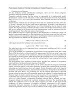
explanation was that it was easier to stay focused for shorter periods of time. Figure 30
shows accuracy data obtained when participants spelled 50 characters of each set of
sequences (12, 10, 8, 6, 4, and 2). As the number of sequences of flashes decrease, the speed
of the BCI system increases as the maximum number of characters read per unit of time
increases. This compromise affects the accuracy of the selected characters. Figure 31 shows
the mean percentages correct for each of the sequences. The percentages are presented as
number of maximum characters per minute.
The results call for the evaluation of the speed accuracy trade-off in an online mode rather

than in an offline analysis to account for the users’ ability to attend to a character over time.
Few potential problems were noticed as follows: Every full scan of a single user input takes
about 15 second, and that might cause a delay in the response of the WMRA system to

change direction on time as the human user wishes. This 15-second delay may cause
problems in case the operator needs to stop the WMRA system for a dangerous situation
such as approaching stairs, or if the user made the wrong selection and needed to return
back to his original choice.


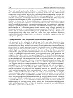
Fig. 29. A person with Guillain-Barre Syndrome driving the WMRA system.


Fig. 30. Accuracy data (% correct) for 6 human subjects.
A9-DoFWheelchair-MountedRoboticArmSystem:
Design,Control,Brain-ComputerInterfacing,andTesting 75

It is important to mention that changing the weights of each of the state variables gives
motion priority to these variables, but may lead to singularity if heavy weights are given to
certain variables when they are necessary for particular motions. For example, when the
seven joints of the arm were given a weight of “1000” and the task required rapid motion of
the arm, singularity occurred since the joints were nearly stationary. Changing these
weights dynamically in the control loop depending on the task in hand leads to a better
performance. This subject will be explored and published in a later publication.


Fig. 25. Manipulability index – using weighted S-R inverse with the gradient projection term
for joint limit avoidance in an extreme case.

6.3 Clinical Testing on Human Subjects

In the teleoperation mode of the testing, several user interfaces were tested. Figure 29 shows
the WMRA system with the Barrette hand installed and a video camera used by a person
affected by Guillain-Barre Syndrome. In her case, she was able to use both the computer
interface and the touch-screen interface. Other user interfaces were tested, but in this paper,
we will discuss the BCI user interface results. When asked, participants informed the tester
that they preferred the 4 and 6 sequences of flashes over the longer sequences. The common
explanation was that it was easier to stay focused for shorter periods of time. Figure 30
shows accuracy data obtained when participants spelled 50 characters of each set of
sequences (12, 10, 8, 6, 4, and 2). As the number of sequences of flashes decrease, the speed
of the BCI system increases as the maximum number of characters read per unit of time
increases. This compromise affects the accuracy of the selected characters. Figure 31 shows
the mean percentages correct for each of the sequences. The percentages are presented as
number of maximum characters per minute.
The results call for the evaluation of the speed accuracy trade-off in an online mode rather
than in an offline analysis to account for the users’ ability to attend to a character over time.
Few potential problems were noticed as follows: Every full scan of a single user input takes
about 15 second, and that might cause a delay in the response of the WMRA system to

change direction on time as the human user wishes. This 15-second delay may cause
problems in case the operator needs to stop the WMRA system for a dangerous situation
such as approaching stairs, or if the user made the wrong selection and needed to return
back to his original choice.


Fig. 29. A person with Guillain-Barre Syndrome driving the WMRA system.


Fig. 30. Accuracy data (% correct) for 6 human subjects.
AdvancesinRobotManipulators76

Fig. 31. Accuracy data (% correct) for each of the flash sequences.

It is also noted that after an extended period of time in using the BCI system, fatigue starts
to appear on the user due to his concentration on the screen when counting the appearances
of his chosen symbol. This tiredness on the user’s side can be a potential problem.
Furthermore, when the user needs to constantly look at the screen and concentrate on the
chosen symbol, This will distract him from looking at where the WMRA is going, and that
poses some danger on the user. Despite the above noted problems, a successful interface
with a good potential for a novel application was developed. Further refinement of the BCI
interface is needed to minimize potential risks.

7. Conclusions and Recommendations

A wheelchair-mounted robotic arm (WMRA) was designed and built to meet the needs of
mobility-impaired persons, and to exceed the capabilities of current devices of this type.
Combining the wheelchair control and the arm control through the augmentation of the
Jacobian to include representations of both resulted in a control system that effectively and
simultaneously controls both devices at once. The control system was designed for
coordinated Cartesian control with singularity robustness and task-optimized combined
mobility and manipulation. Weighted Least Norm solution was implemented to prioritize
the motion between different arm joints and the wheelchair.
Modularity in both the hardware and software levels allowed multiple input devices to be
used to control the system, including the Brain-Computer Interface (BCI). The ability to
communicate a chosen character from the BCI to the controller of the WMRA was presented,
and the user was able to control the motion of WMRA system by focusing attention on a
specific character on the screen. Further testing of different types of displays (e.g.
commands, picture of objects, and a menu display with objects, tasks and locations) is
planned to facilitate communication, mobility and manipulation for people with severe

disabilities. Testing of the control system was conducted in Virtual Reality environment as
well as using the actual hardware developed earlier. The results were presented and
discussed.
The authors would like to thank and acknowledge Dr. Emanuel Donchin, Dr. Yael Arbel,
Dr. Kathryn De Laurentis, and Dr. Eduardo Veras for their efforts in testing the WMRA with
the BCI system. This effort is supported by the National Science Foundation.

8. References

Alqasemi, R.; Mahler, S.; Dubey, R. (2007). “Design and construction of a robotic gripper for
activities of daily living for people with disabilities,” Proceedings of the 2007
ICORR, Noordwijk, the Netherlands, June 13–15.
Alqasemi, R.M.; McCaffrey, E.J.; Edwards, K.D. and Dubey, R.V. (2005). “Analysis,
evaluation and development of wheelchair-mounted robotic arms,” Proceedings of
the 2005 ICORR, Chicago, IL, USA.
Chan, T.F.; Dubey, R.V. (1995). “A weighted least-norm solution based scheme for avoiding
joint limits for redundant joint manipulators,” IEEE Robotics and Automation
Transactions (R&A Transactions 1995). Vol. 11, Issue 2, pp. 286-292.
Chung, J.; Velinsky, S. (1999). “Robust interaction control of a mobile manipulator - dynamic
model based coordination,” Journal of Intelligent and Robotic Systems, Vol. 26, No.
1, pp. 47-63.
Craig, J. (2003). “Introduction to robotics mechanics and control,” Third edition, Addison-
Wesley Publishing, ISBN 0201543613.
Edwards, K.; Alqasemi, R.; Dubey, R. (2006). “Design, construction and testing of a
wheelchair-mounted robotic arm,” Proceedings of the 2006 ICRA, Orlando, FL,
USA.
Eftring, H.; Boschian, K. (1999). “Technical results from manus user trials,” Proceedings of
the 1999 ICORR, 136-141.
Farwell, L.; Donchin, E. (1988). “Talking off the top of your head: Toward a mental
prosthesis utilizing event-related brain potentials,” Electroencephalography and

Clinical Neurophysiology, 70, 510–523.
Galicki, M. (2005). “Control-based solution to inverse kinematics for mobile manipulators
using penalty functions,” 2005 Journal of Intelligent and Robotic Systems, Vol. 42,
No. 3, pp. 213-238.
Luca, A.; Oriolo, G.; Giordano, P. (2006). “Kinematic modeling and redundancy resolution
for nonholonomic mobile manipulators,” Proceedings of the 2006 ICRA, pp. 1867-
1873.
Lüth, T.; Ojdaniæ, D.; Friman, O.; Prenzel, O.; and Gräser, A. (2007). “Low level control in a
semi-autonomous rehabilitation robotic system via a Brain-Computer Interface,”
Proceedings of the 2007 ICORR, Noordwijk, The Netherlands.
Mahoney, R. M. (2001). “The Raptor wheelchair robot system”, Integration of Assistive
Technology in the Information Age. pp. 135-141, IOS, Netherlands.
Nakamura, Y. (1991). “Advanced robotics: redundancy and optimisation,” Addison- Wesley
Publishing, ISBN 0201151987.
Papadopoulos, E.; Poulakakis, J. (2000). “Planning and model-based control for mobile
manipulators,” Proceedings of the 2001 IROS.
A9-DoFWheelchair-MountedRoboticArmSystem:
Design,Control,Brain-ComputerInterfacing,andTesting 77


Fig. 31. Accuracy data (% correct) for each of the flash sequences.

It is also noted that after an extended period of time in using the BCI system, fatigue starts
to appear on the user due to his concentration on the screen when counting the appearances
of his chosen symbol. This tiredness on the user’s side can be a potential problem.
Furthermore, when the user needs to constantly look at the screen and concentrate on the
chosen symbol, This will distract him from looking at where the WMRA is going, and that
poses some danger on the user. Despite the above noted problems, a successful interface
with a good potential for a novel application was developed. Further refinement of the BCI
interface is needed to minimize potential risks.

7. Conclusions and Recommendations

A wheelchair-mounted robotic arm (WMRA) was designed and built to meet the needs of
mobility-impaired persons, and to exceed the capabilities of current devices of this type.
Combining the wheelchair control and the arm control through the augmentation of the
Jacobian to include representations of both resulted in a control system that effectively and
simultaneously controls both devices at once. The control system was designed for
coordinated Cartesian control with singularity robustness and task-optimized combined
mobility and manipulation. Weighted Least Norm solution was implemented to prioritize
the motion between different arm joints and the wheelchair.
Modularity in both the hardware and software levels allowed multiple input devices to be
used to control the system, including the Brain-Computer Interface (BCI). The ability to
communicate a chosen character from the BCI to the controller of the WMRA was presented,
and the user was able to control the motion of WMRA system by focusing attention on a
specific character on the screen. Further testing of different types of displays (e.g.
commands, picture of objects, and a menu display with objects, tasks and locations) is
planned to facilitate communication, mobility and manipulation for people with severe

disabilities. Testing of the control system was conducted in Virtual Reality environment as
well as using the actual hardware developed earlier. The results were presented and
discussed.
The authors would like to thank and acknowledge Dr. Emanuel Donchin, Dr. Yael Arbel,
Dr. Kathryn De Laurentis, and Dr. Eduardo Veras for their efforts in testing the WMRA with
the BCI system. This effort is supported by the National Science Foundation.

8. References

Alqasemi, R.; Mahler, S.; Dubey, R. (2007). “Design and construction of a robotic gripper for
activities of daily living for people with disabilities,” Proceedings of the 2007

ICORR, Noordwijk, the Netherlands, June 13–15.
Alqasemi, R.M.; McCaffrey, E.J.; Edwards, K.D. and Dubey, R.V. (2005). “Analysis,
evaluation and development of wheelchair-mounted robotic arms,” Proceedings of
the 2005 ICORR, Chicago, IL, USA.
Chan, T.F.; Dubey, R.V. (1995). “A weighted least-norm solution based scheme for avoiding
joint limits for redundant joint manipulators,” IEEE Robotics and Automation
Transactions (R&A Transactions 1995). Vol. 11, Issue 2, pp. 286-292.
Chung, J.; Velinsky, S. (1999). “Robust interaction control of a mobile manipulator - dynamic
model based coordination,” Journal of Intelligent and Robotic Systems, Vol. 26, No.
1, pp. 47-63.
Craig, J. (2003). “Introduction to robotics mechanics and control,” Third edition, Addison-
Wesley Publishing, ISBN 0201543613.
Edwards, K.; Alqasemi, R.; Dubey, R. (2006). “Design, construction and testing of a
wheelchair-mounted robotic arm,” Proceedings of the 2006 ICRA, Orlando, FL,
USA.
Eftring, H.; Boschian, K. (1999). “Technical results from manus user trials,” Proceedings of
the 1999 ICORR, 136-141.
Farwell, L.; Donchin, E. (1988). “Talking off the top of your head: Toward a mental
prosthesis utilizing event-related brain potentials,” Electroencephalography and
Clinical Neurophysiology, 70, 510–523.
Galicki, M. (2005). “Control-based solution to inverse kinematics for mobile manipulators
using penalty functions,” 2005 Journal of Intelligent and Robotic Systems, Vol. 42,
No. 3, pp. 213-238.
Luca, A.; Oriolo, G.; Giordano, P. (2006). “Kinematic modeling and redundancy resolution
for nonholonomic mobile manipulators,” Proceedings of the 2006 ICRA, pp. 1867-
1873.
Lüth, T.; Ojdaniæ, D.; Friman, O.; Prenzel, O.; and Gräser, A. (2007). “Low level control in a
semi-autonomous rehabilitation robotic system via a Brain-Computer Interface,”
Proceedings of the 2007 ICORR, Noordwijk, The Netherlands.
Mahoney, R. M. (2001). “The Raptor wheelchair robot system”, Integration of Assistive

Technology in the Information Age. pp. 135-141, IOS, Netherlands.
Nakamura, Y. (1991). “Advanced robotics: redundancy and optimisation,” Addison- Wesley
Publishing, ISBN 0201151987.
Papadopoulos, E.; Poulakakis, J. (2000). “Planning and model-based control for mobile
manipulators,” Proceedings of the 2001 IROS.
AdvancesinRobotManipulators78

Reswick, J.B. (1990). “The moon over dubrovnik - a tale of worldwide impact on persons
with disabilities,” Advances in External Control of Human Extremities.
Schalk, G.; McFarland, D.; Hinterberger, T.; Birbaumer, N.; and Wolpaw, J. (2004). “BCI2000:
A general-purpose brain-computer interface (BCI) system,” IEEE Transactions on
Biomedical Engineering, V. 51, N. 6, pp. 1034-1043.
Sutton, S.; Braren, M.; Zublin, J. and John, E. (1965). “Evoked potential correlates of stimulus
uncertainty,” Science, V. 150, pp. 1187–1188.
US Census Bureau, “Americans with disabilities: 2002,” Census Brief, May 2006,

Valbuena, D.; Cyriacks, M.; Friman, O.; Volosyak, I.; and Gräser, A. (2007). “Brain-computer
interface for high-level control of rehabilitation robotic systems,” Proceedings of
the 2007 ICORR, Noordwijk, The Netherlands.
Yanco, Holly (1998). “Integrating robotic research: a survey of robotic wheelchair
development,” AAAI Spring Symposium on Integrating Robotic Research,
Stanford, California.
Yoshikawa, T. (1990). “Foundations of robotics: analysis and control,” MIT Press, ISBN
0262240289.
AdvancedTechniquesofIndustrialRobotProgramming 79
AdvancedTechniquesofIndustrialRobotProgramming
FrankShaopengCheng
x

Advanced Techniques

of Industrial Robot Programming


Frank Shaopeng Cheng
Central Michigan University
United States

1. Introduction

Industrial robots are reprogrammable, multifunctional manipulators designed to move
parts, materials, and devices through computer controlled motions. A robot application
program is a set of instructions that cause the robot system to move the robot’s end-of-arm-
tooling (or end-effector) to robot points for performing the desired robot tasks. Creating
accurate robot points for an industrial robot application is an important programming task.
It requires a robot programmer to have the knowledge of the robot’s reference frames,
positions, software operations, and the actual programming language. In the conventional
“lead-through” method, the robot programmer uses the robot teach pendant to position the
robot joints and end-effector via the actual workpiece and record the satisfied robot pose as
a robot point. Although the programmer’s visual observations can make the taught robot
points accurate, the required teaching task has to be conducted with the real robot online
and the taught points can be inaccurate if the positions of the robot’s end-effector and
workpiece are slightly changed in the robot operations. Other approaches have been utilized
to reduce or eliminate these limitations associated with the online robot programming. This
includes generating or recovering robot points through user-defined robot frames, external
measuring systems, and robot simulation software (Cheng, 2003; Connolly, 2006;
Pulkkinen1 et al., 2008; Zhang et al., 2006).
Position variations of the robot’s end-effector and workpiece in the robot operations are
usually the reason for inaccuracy of the robot points in a robot application program. To
avoid re-teaching all the robot points, the robot programmer needs to identify these position
variations and modify the robot points accordingly. The commonly applied techniques

include setting up the robot frames and measuring their positional offsets through the robot
system, an external robot calibration system (Cheng, 2007), or an integrated robot vision
system (Cheng, 2009; Connolly, 2007). However, the applications of these measuring and
programming techniques require the robot programmer to conduct the integrated design
tasks that involve setting up the functions and collecting the measurements in the
measuring systems. Misunderstanding these concepts or overlooking these steps in the
design technique will cause the task of modifying the robot points to be ineffective.
Robot production downtime is another concern with online robot programming. Today’s
robot simulation software provides the robot programmer with the functions of creating
4
AdvancesinRobotManipulators80

virtual robot points and programming virtual robot motions in an interactive and virtual 3D
design environment (Cheng, 2003; Connolly, 2006). By the time a robot simulation design is
completed, the simulation robot program is able to move the virtual robot and end-effector
to all desired virtual robot points for performing the specified operations to the virtual
workpiece without collisions in the simulated workcell. However, because of the inevitable
dimensional differences of the components between the real robot workcell and the
simulated robot workcell, the virtual robot points created in the simulated workcell must be
adjusted relative to the actual position of the components in the real robot workcell before
they can be downloaded to the real robot system. This task involves the techniques of
calibrating the position coordinates of the simulation Device models with respect to the
user-defined real robot points.
In this chapter, advanced techniques used in creating industrial robot points are discussed
with the applications of the FANUC robot system, Delmia IGRIP robot simulation software,
and Dynalog DynaCal robot calibration system. In Section 2, the operation and
programming of an industrial robot system are described. This includes the concepts of
robot’s frames, positions, kinematics, motion segments, and motion instructions. The
procedures for teaching robot frames and robot points online with the real robot system are
introduced. Programming techniques for maintaining the accuracy of the exiting robot

points are also discussed. Section 3 introduces the setup and integration of a two
dimensional (2D) vision system for performing vision-guided robot operations. This
includes establishing integrated measuring functions in both robot and vision systems and
modifying existing robot points through vision measurements for vision-identified
workpieces. Section 4 discusses the robot simulation and offline programming techniques.
This includes the concepts and procedures related to creating virtual robot points and
enhancing their accuracy for a real robot system. Section 5 explores the techniques for
transferring industrial robot points between two identical robot systems and the methods
for enhancing the accuracy of the transferred robot points through robot system calibration.
A summary is then presented in Section 6.

2. Creating Robot Points Online with Robot

The static positions of an industrial robot are represented by Cartesian reference frames and
frame transformations. Among them, the robot base frame R(x, y, z) is a fixed one and the
robot’s default tool-center-point frame Def_TCP (n, o, a), located at the robot’s wrist
faceplate, is a moving one. The position of frame Def_TCP relative to frame R is defined as
the robot point
R
TCP_Def
]n[P
and is mathematically determined by the 4  4 homogeneous
transformation matrix in Eq. (1)















1000
paon
paon
paon
T]n[P
zzzz
yyyy
xxxx
TCP_Def
RR
TCP_Def
, (1)

where the coordinates of vector p = (p
x
, p
y
, p
z
) represent the location of frame Def_TCP and
the coordinates of three unit directional vectors n, o, and a represent the orientation of frame

Def_TCP. The inverse of

R
T
Def_TCP
or
R
TCP_Def
]n[P
denoted as (
R
T
Def_TCP
)
-1
or (
R
TCP_Def
]n[P
)
-1

represents the position of frame R to frame Def_TCP, which is equal to frame transformation
Def_TCP
T
R
. Generally, the definition of a frame transformation matrix or its inverse described
above can be applied for measuring the relative position between any two frames in the
robot system (Niku, 2001). The orientation coordinates of frame Def_TCP in Eq. (1) can be
determined by Eq. (2)


























xyxyy
xzxyzxzxyzyz
xzxyzxzxyzyz
xyz
zzz

yyy
xxx
coscossincossin
sincoscossinsincoscossinsinsincossin
sinsincossincoscossinsinsincoscoscos
),x(Rot),y(Rot),z(Rot
aon
aon
aon
, (2)

where transformations Rot(x, θ
x
), Rot(y, θ
y
), and Rot(z, θ
z
) are pure rotations of frame
Def_TCP about the x-, y-, and z-axes of frame R with the angles of θ
x
(yaw), θ
y
(pitch), and θ
z

(roll), respectively. Thus, a robot point
R
TCP_Def
]n[P
can also be represented by Cartesian

coordinates in Eq. (3)


)r,p,w,z,y,x(]n[P
R
TCP_Def

. (3)

It is obvious that the robot’s joint movements are to change the position of frame Def_TCP.
For an n-joint robot, the geometric motion relationship between the Cartesian coordinates of
a robot point
R
TCP_Def
]n[P
in frame R (i.e. the robot world space) and the proper
displacements of its joint variables q = (q
1
, q
2
, q
n
) in robot joint frames (i.e. the robot joint
space) is mathematically modeled as the robot’s kinematics equations in Eq. (4)




























1000
)r,q(f)r,q(f)r,q(f)r,q(f
)r,q(f)r,q(f)r,q(f)r,q(f
)r,q(f)r,q(f)r,q(f)r,q(f
1000
paon
paon
paon
34333231

24232221
14131211
zzzz
yyyy
xxxx
, (4)

where f
ij
(q, r) (for i = 1, 2, 3 and j = 1, 2, 3, 4) is a function of joint variables q and joint
parametersr.
Specifically, the robot forward kinematics equations will enable the robot system to determine
where a
R
TCP_Def
]n[P
will be if the displacements of all joint variables q=(q
1
, q
2
, q
n
) are known.
The robot inverse kinematics equations will enable the robot system to calculate what
displacement of each joint variable q
k
(for k = 1 , , n) must be if a
R
TCP_Def
]n[P

is specified. If the
inverse kinematics solutions for a given
R
TCP_Def
]n[P
are infinite, the robot system defines the point
as a robot “singularity” and cannot move frame Def_TCP to it.
AdvancedTechniquesofIndustrialRobotProgramming 81

virtual robot points and programming virtual robot motions in an interactive and virtual 3D
design environment (Cheng, 2003; Connolly, 2006). By the time a robot simulation design is
completed, the simulation robot program is able to move the virtual robot and end-effector
to all desired virtual robot points for performing the specified operations to the virtual
workpiece without collisions in the simulated workcell. However, because of the inevitable
dimensional differences of the components between the real robot workcell and the
simulated robot workcell, the virtual robot points created in the simulated workcell must be
adjusted relative to the actual position of the components in the real robot workcell before
they can be downloaded to the real robot system. This task involves the techniques of
calibrating the position coordinates of the simulation Device models with respect to the
user-defined real robot points.
In this chapter, advanced techniques used in creating industrial robot points are discussed
with the applications of the FANUC robot system, Delmia IGRIP robot simulation software,
and Dynalog DynaCal robot calibration system. In Section 2, the operation and
programming of an industrial robot system are described. This includes the concepts of
robot’s frames, positions, kinematics, motion segments, and motion instructions. The
procedures for teaching robot frames and robot points online with the real robot system are
introduced. Programming techniques for maintaining the accuracy of the exiting robot
points are also discussed. Section 3 introduces the setup and integration of a two
dimensional (2D) vision system for performing vision-guided robot operations. This
includes establishing integrated measuring functions in both robot and vision systems and

modifying existing robot points through vision measurements for vision-identified
workpieces. Section 4 discusses the robot simulation and offline programming techniques.
This includes the concepts and procedures related to creating virtual robot points and
enhancing their accuracy for a real robot system. Section 5 explores the techniques for
transferring industrial robot points between two identical robot systems and the methods
for enhancing the accuracy of the transferred robot points through robot system calibration.
A summary is then presented in Section 6.

2. Creating Robot Points Online with Robot

The static positions of an industrial robot are represented by Cartesian reference frames and
frame transformations. Among them, the robot base frame R(x, y, z) is a fixed one and the
robot’s default tool-center-point frame Def_TCP (n, o, a), located at the robot’s wrist
faceplate, is a moving one. The position of frame Def_TCP relative to frame R is defined as
the robot point
R
TCP_Def
]n[P
and is mathematically determined by the 4  4 homogeneous
transformation matrix in Eq. (1)















1000
paon
paon
paon
T]n[P
zzzz
yyyy
xxxx
TCP_Def
RR
TCP_Def
, (1)

where the coordinates of vector p = (p
x
, p
y
, p
z
) represent the location of frame Def_TCP and
the coordinates of three unit directional vectors n, o, and a represent the orientation of frame

Def_TCP. The inverse of
R
T
Def_TCP

or
R
TCP_Def
]n[P
denoted as (
R
T
Def_TCP
)
-1
or (
R
TCP_Def
]n[P
)
-1

represents the position of frame R to frame Def_TCP, which is equal to frame transformation
Def_TCP
T
R
. Generally, the definition of a frame transformation matrix or its inverse described
above can be applied for measuring the relative position between any two frames in the
robot system (Niku, 2001). The orientation coordinates of frame Def_TCP in Eq. (1) can be
determined by Eq. (2)




























xyxyy
xzxyzxzxyzyz
xzxyzxzxyzyz
xyz
zzz
yyy
xxx
coscossincossin

sincoscossinsincoscossinsinsincossin
sinsincossincoscossinsinsincoscoscos
),x(Rot),y(Rot),z(Rot
aon
aon
aon
, (2)

where transformations Rot(x, θ
x
), Rot(y, θ
y
), and Rot(z, θ
z
) are pure rotations of frame
Def_TCP about the x-, y-, and z-axes of frame R with the angles of θ
x
(yaw), θ
y
(pitch), and θ
z

(roll), respectively. Thus, a robot point
R
TCP_Def
]n[P
can also be represented by Cartesian
coordinates in Eq. (3)

)r,p,w,z,y,x(]n[P
R
TCP_Def

. (3)

It is obvious that the robot’s joint movements are to change the position of frame Def_TCP.
For an n-joint robot, the geometric motion relationship between the Cartesian coordinates of
a robot point
R
TCP_Def
]n[P
in frame R (i.e. the robot world space) and the proper
displacements of its joint variables q = (q
1
, q
2
, q
n
) in robot joint frames (i.e. the robot joint
space) is mathematically modeled as the robot’s kinematics equations in Eq. (4)




























1000
)r,q(f)r,q(f)r,q(f)r,q(f
)r,q(f)r,q(f)r,q(f)r,q(f
)r,q(f)r,q(f)r,q(f)r,q(f
1000
paon
paon
paon
34333231
24232221
14131211
zzzz

yyyy
xxxx
, (4)

where f
ij
(q, r) (for i = 1, 2, 3 and j = 1, 2, 3, 4) is a function of joint variables q and joint
parametersr.
Specifically, the robot forward kinematics equations will enable the robot system to determine
where a
R
TCP_Def
]n[P
will be if the displacements of all joint variables q=(q
1
, q
2
, q
n
) are known.
The robot inverse kinematics equations will enable the robot system to calculate what
displacement of each joint variable q
k
(for k = 1 , , n) must be if a
R
TCP_Def
]n[P
is specified. If the
inverse kinematics solutions for a given
R

TCP_Def
]n[P
are infinite, the robot system defines the point
as a robot “singularity” and cannot move frame Def_TCP to it.
AdvancesinRobotManipulators82

In robot programming, the robot programmer creates a robot point
R
TCP_Def
]n[P
by first declaring
it in a robot program and then defining its coordinates in the robot system. The conventional
method is through recording a particular robot pose with the robot teach pendent (Rehg, 2003).
Under the teaching mode, the robot programmer jogs the robot’s joints for poisoning the robot’s
end-effector relative to the workpiece. As joint k moves, the serial pulse coder of the joint
measures the joint displacement q
k
relative to the “zero” position of the joint frame. The robot
system substitutes all measured values of q = (q
1
, q
2
, q
n
) into the robot forward kinematics
equations to determine the corresponding Cartesian coordinates of frame Def_TCP in Eq. (1) and
Eq. (3). After the robot programmer records a
R
TCP_Def
]n[P

with the teach pendant, its Cartesian
coordinates and the corresponding joint values are saved in the robot system. The robot
programmer may use the “Representation” softkey on the teach pendant to automatically
convert and display the joint values and Cartesian coordinates of a taught robot point
R
TCP_Def
]n[P
. It is important to notice that Cartesian coordinates in Eq. (3) is the standard
representation of a
R
TCP_Def
]n[P
in the industrial robot system, and its joint representation always
uniquely defines the position of frame Def_TCP (i.e. the robot pose) in frame R.
In robot programming, the robot programmer defines a motion segment of frame Def_TCP by
using two taught robot points in a robot motion instruction. During the execution of a motion
instruction, the robot system utilizes the trajectory planning method called “linear segment with
parabolic blends” to control the joint motion and implement the actual trajectory of frame
Def_TCP through one of the two user-specified motion types. The “joint” motion type allows the
robot system to start and end the motion of all robot joints at the same time resulting in an
unpredictable, but repeatable trajectory for frame Def_TCP. The “Cartesian” motion type allows
the robot system to move frame Def_TCP along a user-specified Cartesian path such as a straight
line or a circular arc in frame R during the motion segment, which is implemented in three steps.
First, the robot system interpolates a number of intermediate points along the specified Cartesian
path in the motion segment. Then, the proper joint values for each interpolated robot point are
calculated by the robot inverse kinematics equations. Finally, the “joint” motion type is applied
to move the robot joints between two consecutive interpolated robot points.
Different robot languages provide the robot systems with motion instructions in different format.
The motion instruction of FANUC Teach Pendant Programming (TPP) language (Fanuc, 2007)
allows the robot programmer to define a motion segment in one statement that includes the

robot point P[n], motion type, speed, motion termination type, and associated motion options.
Table 1 shows two motion instructions used in a FANUC TP program.

FANUC TPP Instruction Description
1. J P[1] 50% FINE

Moves the TCP frame to robot point P[1]
with “Joint” motion type (J) and at 50% of
the default joint maximum speed, and stops
exactly at P[1] with a “Fine” motion
termination.

2. L P[2] 100 mm/sec FINE

Utilizes “Linear” motion type (L) to move
TCP frame along a straight line from P[1] to
P[2] with a TCP speed of 100 mm/sec and a
“Fine” motion termination type.

Table 1. Motion instructions of FANUC TPP language

2.1 Design of Robot User Tool Frame
In the industrial robot system, the robot programmer can define a robot user tool frame
UT[k](x, y, z) relative to frame Def_TCP for representing the actual tool-tip point of the
robot’s end-effector. Usually, the UT[k] origin represents the tool-tip point and the z-axis
represents the tool axis. A UT[k] plays an important role in robot programming as it not
only defines the actual tool-tip point but also addresses its variations. Thus, every end-
effector used in a robot application must be defined as a UT[k] and saved in robot system
variable UTOOL[k]. Practically, the robot programmer may directly define and select a
UT[k] within a robot program or from the robot teach pendant. Table 2 shows the UT[k]

frame selection instructions of FANUC TPP language. When the coordinates of a UT[k] is
set to zero, it represents frame Def_TCP. The robot system uses the current active UT[k] to
record a robot point
R
]k[UT
]n[P
as shown in Eq. (5) and cannot move the robot to any robot
point
R
]g[UT
]m[P
that is taught with a UT[g] different from UT[k] (i.e. g ≠ k).

]k[UT
RR
]k[UT
T]n[P 
(5)

It is obvious that a robot point
R
TCP_Def
]n[P
in Eq. (1) or Eq. (3) can be taught with different
UT[k], thus, represented in different Cartesian coordinates in the robot system as shown in
Eq. (6)


]k[UT
TCP_DefR

TCP_Def
R
]k[UT
T]n[P]n[P 
. (6)

FANUC TPP Instruction Description
1.
UTOOL_NUM=1

Set UT[1] frame to be the current active
UT.
Table 2. UT[k] frame selection instructions of FANUC TPP language

To define a UT[k] for an actual tool-tip point P
T-Ref
whose coordinates (x, y, z, w, p, r) in
frame D
ef_TCP
is unknown, the robot programmer must follow the UT Frame Setup
procedure provided by the robot system and teach six robot points
R
TCP_Def
]n[P

(for n = 1, 2, … 6) with respect to P
T-Ref
and a reference point P
S-Ref
on a tool reachable

surface. The “three-point” method as shown in Eq. (7) and Eq. (8) utilizes the first three
taught robot points in the UT Frame Setup procedure to determine the UT[k] origin.
Suppose that the coordinates of vector
Def_TCP
p= [p
n
, p
o
, p
a
]
T
represent point P
T-Ref
in frame
Def_TCP. Then, it can be determined in Eq. (7)


p)T(p
R1
1
TCP_Def


, (7)

where the coordinates of vector
R
p= [p
x

, p
y
, p
z
]
T
represents point P
T-Ref
in frame R and T
1

represents the first taught robot point
R
TCP_Def
]1[P
when point P
T-Ref
touches point P
S-Ref
. The
coordinates of vector
R
p= [p
x
, p
y
, p
z
]
T

also represents point P
S-Ref
in frame R and can be
solved by the three linear equations in Eq. (8)

AdvancedTechniquesofIndustrialRobotProgramming 83

In robot programming, the robot programmer creates a robot point
R
TCP_Def
]n[P
by first declaring
it in a robot program and then defining its coordinates in the robot system. The conventional
method is through recording a particular robot pose with the robot teach pendent (Rehg, 2003).
Under the teaching mode, the robot programmer jogs the robot’s joints for poisoning the robot’s
end-effector relative to the workpiece. As joint k moves, the serial pulse coder of the joint
measures the joint displacement q
k
relative to the “zero” position of the joint frame. The robot
system substitutes all measured values of q = (q
1
, q
2
, q
n
) into the robot forward kinematics
equations to determine the corresponding Cartesian coordinates of frame Def_TCP in Eq. (1) and
Eq. (3). After the robot programmer records a
R
TCP_Def

]n[P
with the teach pendant, its Cartesian
coordinates and the corresponding joint values are saved in the robot system. The robot
programmer may use the “Representation” softkey on the teach pendant to automatically
convert and display the joint values and Cartesian coordinates of a taught robot point
R
TCP_Def
]n[P
. It is important to notice that Cartesian coordinates in Eq. (3) is the standard
representation of a
R
TCP_Def
]n[P
in the industrial robot system, and its joint representation always
uniquely defines the position of frame Def_TCP (i.e. the robot pose) in frame R.
In robot programming, the robot programmer defines a motion segment of frame Def_TCP by
using two taught robot points in a robot motion instruction. During the execution of a motion
instruction, the robot system utilizes the trajectory planning method called “linear segment with
parabolic blends” to control the joint motion and implement the actual trajectory of frame
Def_TCP through one of the two user-specified motion types. The “joint” motion type allows the
robot system to start and end the motion of all robot joints at the same time resulting in an
unpredictable, but repeatable trajectory for frame Def_TCP. The “Cartesian” motion type allows
the robot system to move frame Def_TCP along a user-specified Cartesian path such as a straight
line or a circular arc in frame R during the motion segment, which is implemented in three steps.
First, the robot system interpolates a number of intermediate points along the specified Cartesian
path in the motion segment. Then, the proper joint values for each interpolated robot point are
calculated by the robot inverse kinematics equations. Finally, the “joint” motion type is applied
to move the robot joints between two consecutive interpolated robot points.
Different robot languages provide the robot systems with motion instructions in different format.
The motion instruction of FANUC Teach Pendant Programming (TPP) language (Fanuc, 2007)

allows the robot programmer to define a motion segment in one statement that includes the
robot point P[n], motion type, speed, motion termination type, and associated motion options.
Table 1 shows two motion instructions used in a FANUC TP program.

FANUC TPP Instruction Description
1.
J P[1] 50% FINE

Moves the TCP frame to robot point P[1]
with “Joint” motion type (J) and at 50% of
the default joint maximum speed, and stops
exactly at P[1] with a “Fine” motion
termination.

2. L P[2] 100 mm/sec FINE

Utilizes “Linear” motion type (L) to move
TCP frame along a straight line from P[1] to
P[2] with a TCP speed of 100 mm/sec and a
“Fine” motion termination type.

Table 1. Motion instructions of FANUC TPP language

2.1 Design of Robot User Tool Frame
In the industrial robot system, the robot programmer can define a robot user tool frame
UT[k](x, y, z) relative to frame Def_TCP for representing the actual tool-tip point of the
robot’s end-effector. Usually, the UT[k] origin represents the tool-tip point and the z-axis
represents the tool axis. A UT[k] plays an important role in robot programming as it not
only defines the actual tool-tip point but also addresses its variations. Thus, every end-
effector used in a robot application must be defined as a UT[k] and saved in robot system

variable UTOOL[k]. Practically, the robot programmer may directly define and select a
UT[k] within a robot program or from the robot teach pendant. Table 2 shows the UT[k]
frame selection instructions of FANUC TPP language. When the coordinates of a UT[k] is
set to zero, it represents frame Def_TCP. The robot system uses the current active UT[k] to
record a robot point
R
]k[UT
]n[P
as shown in Eq. (5) and cannot move the robot to any robot
point
R
]g[UT
]m[P
that is taught with a UT[g] different from UT[k] (i.e. g ≠ k).

]k[UT
RR
]k[UT
T]n[P 
(5)

It is obvious that a robot point
R
TCP_Def
]n[P
in Eq. (1) or Eq. (3) can be taught with different
UT[k], thus, represented in different Cartesian coordinates in the robot system as shown in
Eq. (6)

]k[UT
TCP_DefR
TCP_Def
R
]k[UT
T]n[P]n[P 
. (6)

FANUC TPP Instruction Description
1. UTOOL_NUM=1

Set UT[1] frame to be the current active
UT.
Table 2. UT[k] frame selection instructions of FANUC TPP language

To define a UT[k] for an actual tool-tip point P
T-Ref
whose coordinates (x, y, z, w, p, r) in
frame D
ef_TCP
is unknown, the robot programmer must follow the UT Frame Setup
procedure provided by the robot system and teach six robot points
R
TCP_Def
]n[P

(for n = 1, 2, … 6) with respect to P
T-Ref
and a reference point P
S-Ref

on a tool reachable
surface. The “three-point” method as shown in Eq. (7) and Eq. (8) utilizes the first three
taught robot points in the UT Frame Setup procedure to determine the UT[k] origin.
Suppose that the coordinates of vector
Def_TCP
p= [p
n
, p
o
, p
a
]
T
represent point P
T-Ref
in frame
Def_TCP. Then, it can be determined in Eq. (7)


p)T(p
R1
1
TCP_Def


, (7)

where the coordinates of vector
R
p= [p

x
, p
y
, p
z
]
T
represents point P
T-Ref
in frame R and T
1

represents the first taught robot point
R
TCP_Def
]1[P
when point P
T-Ref
touches point P
S-Ref
. The
coordinates of vector
R
p= [p
x
, p
y
, p
z
]

T
also represents point P
S-Ref
in frame R and can be
solved by the three linear equations in Eq. (8)

AdvancesinRobotManipulators84


0p)TTI(
R1
32


, (8)

where transformations T
2
and T
3
represent the other two taught robot points
R
TCP_Def
]2[P
and
R
TCP_Def
]3[P
in the UT Frame Setup procedure respectively when point P
T-Ref

is at point P
S-Ref
.
To ensure the UT[k] accuracy, these three robot points must be taught with point P
T-Ref

touching point P
S-Ref
from three different approach statuses. Practically,
R
TCP_Def
]2[P
(or
R
TCP_Def
]3[P
) can be taught by first rotating frame Def_TCP about its x-axis (or y-axis) for at
least 90 degrees (or 60 degrees) when the tool is at
R
TCP_Def
]1[P
, and then moving point P
T-Ref

back to point P
S-Ref
. A UT[k] taught with the “three-point” method has the same orientation
of frame Def_TCP.

Surface

Reference Point
Tool-tip
Reference Point

Fig. 1. The three-point method in teaching a UT[k]

If the UT[k] orientation needs to be defined differently from frame Def_TCP, the robot
programmer must use the “six-point” method and teach additional three robot points
required in UT Frame Setup procedure. These three points define the orient origin point, the
positive x-direction, and the positive z-direction of the UT[k], respectively. The method of
using such three non-collinear robot points for determining the orientation of a robot frame
is to be discussed in section 2.2.
Due to the tool change or damage in robot operations the actual tool-tip point of a robot’s
end-effector can be varied from its taught UT[k], which causes the inaccuracy of existing
robot points relative to the workpiece. To aviod re-teaching all robot points, the robot
programmer needs to teach a new UT[k]’ for the changed tool-tip point and shift all existing
robot points through offset
Def_TCP
T
Def_TCP’
as shown in Fig. 2. Assume that transformation
Def_TCP
T
UT[k]
represents the position of the original tool-tip point and remains unchanged
when frame UT[k] changes into new UT[k]’ as shown in Eq. (9)


]'k[UT
'TCP_Def

]k[UT
TCP_Def
TT 
, (9)

where frame Def_TCP‘ represents the position of frame Def_TCP after frame UT[k] moves

to UT[k]’. In this case, the pre-taught robot point
R
]k[UT
]n[P
can be shifted into the
corresponding robot point
R
]'k[UT
]n[P
through Eq. (10)


]'k[UT
'TCP_Def
'TCP_Def
TCP_Def
]'k[UT
TCP_Def
TTT 
. (10)

The industrial robot system usually implements Eq. (9) and Eq. (10) as both a system utility
function and a program instruction. As a system utility function, the offset

Def_TCP
T
Def_TCP’

changes the position of frame Def_TCP in the robot system so that the robot programmer is
able to change the current UT[k] of a taught P[n] into a different UT[k]’ while remaining the
same Cartesian coordinates of P[n] in frame R. As a program instruction,
Def_TCP
T
Def_TCP’

shifts the pre-taught robot point
R
]k[UT
]n[P
into the corresponding point
R
]'k[UT
]'n[P
without
changing the position of frame Def_TCP. Table 3 shows the UT[k] offset instruction of
FANUC TPP language for Eq. (10).

]'k[UT
'TCP_Def
T
'TCP_Def
TCP_Def
T
]k[UT

TCP_Def
T
]'k[UT
TCP_Def
T


Fig. 2. Shifting a robot point through the offset of frame Def_TCP

TP Instructions Description
1. Tool_Offset Conditions PR[x], UTOOL[k],

Offset value
Def_TCP
T
Def_TCP’
is
stored in a user-specified position
register PR[x].
2. J P[n] 100% Fine Tool_Offset

The “Offset” option in motion
instruction shifts the existing
robot point
R
]k[UT
]n[P
into
corresponding point
R

]'k[UT
]'n[P
.
Table 3. UT[k] offset instruction of FANUC TPP language

2.2 Design of Robot User Frame
In the industrial robot system, the robot programmer is able to establish a robot user frame
UF[i](x, y, z) relative to frame R and save it in robot system variable UFRAME[i]. A defined
UF[i] can be selected within a robot program or from the robot teach pendant. The robot
system uses the current active UF[i] to record robot point
]i[UF
]k[UT
]n[P
as shown in Eq. (11) and
AdvancedTechniquesofIndustrialRobotProgramming 85


0p)TTI(
R1
32


, (8)

where transformations T
2
and T
3
represent the other two taught robot points
R

TCP_Def
]2[P
and
R
TCP_Def
]3[P
in the UT Frame Setup procedure respectively when point P
T-Ref
is at point P
S-Ref
.
To ensure the UT[k] accuracy, these three robot points must be taught with point P
T-Ref

touching point P
S-Ref
from three different approach statuses. Practically,
R
TCP_Def
]2[P
(or
R
TCP_Def
]3[P
) can be taught by first rotating frame Def_TCP about its x-axis (or y-axis) for at
least 90 degrees (or 60 degrees) when the tool is at
R
TCP_Def
]1[P
, and then moving point P

T-Ref

back to point P
S-Ref
. A UT[k] taught with the “three-point” method has the same orientation
of frame Def_TCP.

Surface
Reference Point
Tool-tip
Reference Point

Fig. 1. The three-point method in teaching a UT[k]

If the UT[k] orientation needs to be defined differently from frame Def_TCP, the robot
programmer must use the “six-point” method and teach additional three robot points
required in UT Frame Setup procedure. These three points define the orient origin point, the
positive x-direction, and the positive z-direction of the UT[k], respectively. The method of
using such three non-collinear robot points for determining the orientation of a robot frame
is to be discussed in section 2.2.
Due to the tool change or damage in robot operations the actual tool-tip point of a robot’s
end-effector can be varied from its taught UT[k], which causes the inaccuracy of existing
robot points relative to the workpiece. To aviod re-teaching all robot points, the robot
programmer needs to teach a new UT[k]’ for the changed tool-tip point and shift all existing
robot points through offset
Def_TCP
T
Def_TCP’
as shown in Fig. 2. Assume that transformation
Def_TCP

T
UT[k]
represents the position of the original tool-tip point and remains unchanged
when frame UT[k] changes into new UT[k]’ as shown in Eq. (9)


]'k[UT
'TCP_Def
]k[UT
TCP_Def
TT 
, (9)

where frame Def_TCP‘ represents the position of frame Def_TCP after frame UT[k] moves

to UT[k]’. In this case, the pre-taught robot point
R
]k[UT
]n[P
can be shifted into the
corresponding robot point
R
]'k[UT
]n[P
through Eq. (10)


]'k[UT
'TCP_Def
'TCP_Def

TCP_Def
]'k[UT
TCP_Def
TTT 
. (10)

The industrial robot system usually implements Eq. (9) and Eq. (10) as both a system utility
function and a program instruction. As a system utility function, the offset
Def_TCP
T
Def_TCP’

changes the position of frame Def_TCP in the robot system so that the robot programmer is
able to change the current UT[k] of a taught P[n] into a different UT[k]’ while remaining the
same Cartesian coordinates of P[n] in frame R. As a program instruction,
Def_TCP
T
Def_TCP’

shifts the pre-taught robot point
R
]k[UT
]n[P
into the corresponding point
R
]'k[UT
]'n[P
without
changing the position of frame Def_TCP. Table 3 shows the UT[k] offset instruction of
FANUC TPP language for Eq. (10).

]'k[UT
'TCP_Def
T
'TCP_Def
TCP_Def
T
]k[UT
TCP_Def
T
]'k[UT
TCP_Def
T


Fig. 2. Shifting a robot point through the offset of frame Def_TCP

TP Instructions Description
1. Tool_Offset Conditions PR[x], UTOOL[k],

Offset value
Def_TCP
T
Def_TCP’
is
stored in a user-specified position
register PR[x].
2. J P[n] 100% Fine Tool_Offset

The “Offset” option in motion

instruction shifts the existing
robot point
R
]k[UT
]n[P
into
corresponding point
R
]'k[UT
]'n[P
.
Table 3. UT[k] offset instruction of FANUC TPP language

2.2 Design of Robot User Frame
In the industrial robot system, the robot programmer is able to establish a robot user frame
UF[i](x, y, z) relative to frame R and save it in robot system variable UFRAME[i]. A defined
UF[i] can be selected within a robot program or from the robot teach pendant. The robot
system uses the current active UF[i] to record robot point
]i[UF
]k[UT
]n[P
as shown in Eq. (11) and
AdvancesinRobotManipulators86

cannot move the robot to any robot point
]j[UF
]k[UT
]m[P
that is taught with a UF[j] different
from UF[i] (i.e. j ≠ i).

]k[UT
]i[UF]i[UF
]k[UT
T]n[P 
. (11)

It is obvious that a robot point
R
TCP_Def
]n[P
in Eq. (1) or Eq. (3) can be taught with different
UT [k] and UF[i], thus, represented in different Cartesian coordinates in the robot system as
shown in Eq. (12)


]k[UT
TCP_DefR
TCP_Def
1
]i[UF
R]i[UF
]k[UT
T]n[P)T(]n[P 

. (12)

However, the joint representation of a
R

TCP_Def
]n[P
uniquely defines the robot pose.
The robot programmer can directly define a UF[i] with a known robot position measured in
frame R. Table 4 shows the UF[i] setup instructions of FANUC TPP language.

FANUC TPP Instructions Description
1. UFRAME[i]=PR[x]

Assign the value of a robot position
register PR[x] to UF[i]
2. UFRAME[i]=LPOS

Assign the current coordinates of frame
Def_TCP to UF[i]
3. UFRAME_NUM= i Set UF[i] to be active in the robot system
Table 4. UF[i] setup instructions of FANUC TPP language

However, to define a UF[i] at a position whose coordinates (x, y, z, w, p, r) in frame R is
unknown, the robot programmer needs to follow the UF Setup procedure provided by the
robot system and teach four specially defined points
R
]k[UT
]n[P
(for n = 1, 2, … 4) where
UT[k] represents the tool-tip point of a pointer. In this method as shown in Fig. 3, the
location coordinates (x, y, z) of P[4] (i.e. the system-origin point) defines the actual UF[i]
origin. The robot system defines the x-, y- and z-axes of frame UF[i] through three mutually
perpendicular unit vectors a, b, and c as shown in Eq. (13)



 bac
, (13)

where the coordinates of vectors a and b are determined by the location coordinates (x, y, z)
of robot points P[1] (i.e. the positive x-direction point), P[2] (i.e. the positive y-direction
point), and P[3] (i.e. the system orient-origin point) in R frame as shown in Fig. 3.
With a taught UF[i], the robot programmer is able to teach a group of robot points relative to
it and shift the taught points through its offset value. Fig. 4 shows the method for shifting a
taught robot point
]i[UF
]k[UT
]n[P
with the offset of UF[i].



Fig. 3. The four-point method in teaching a UF[i]

]'k[UT
]'i[UF
T
]'i[UF
]i[UF
T
]k[UT
]i[UF
T

]'k[UT
]i[UF
T

Fig. 4. Shifting a robot point through the offset of UF[i]

Assume that transformation
UF[i]
T
UT[k]
represents a taught robot point P[n] and remains
unchanged when P[n] shifts to P[n]’ as shown in Eq. (14)


]'k[UT
]'i[UF
]k[UT
]i[UF
TT 

or (14)

]'i[UF
]'k[UT
]i[UF
]k[UT
]'n[P]n[P 
,

where frame UF[i]‘ represents the position of frame UF[i] after P[n] becomes P[n]’. Also,

assume that transformation
UF[i]
T
UF[i]’
represents the position change of UF[i]’ relative to
UF[i], thus, transformation
UF[i]
T
UT[k]
(or robot point
]i[UF
]k[UT
]n[P
) can be converted (or shifted)
to
UF[i]
T
UT[k]’
(or
]i[UF
]'k[UT
]'n[P
) as shown in Eq. (15)


]'k[UT
]'i[UF
]'i[UF
]i[UF
]'k[UT

]i[UF
TTT 

or (15)

]i[UF
]k[UT
]'i[UF
]i[UF]i[UF
]'k[UT
]n[PT]'n[P 
.
AdvancedTechniquesofIndustrialRobotProgramming 87

cannot move the robot to any robot point
]j[UF
]k[UT
]m[P
that is taught with a UF[j] different
from UF[i] (i.e. j ≠ i).


]k[UT
]i[UF]i[UF
]k[UT
T]n[P 
. (11)

It is obvious that a robot point
R

TCP_Def
]n[P
in Eq. (1) or Eq. (3) can be taught with different
UT [k] and UF[i], thus, represented in different Cartesian coordinates in the robot system as
shown in Eq. (12)


]k[UT
TCP_DefR
TCP_Def
1
]i[UF
R]i[UF
]k[UT
T]n[P)T(]n[P 

. (12)

However, the joint representation of a
R
TCP_Def
]n[P
uniquely defines the robot pose.
The robot programmer can directly define a UF[i] with a known robot position measured in
frame R. Table 4 shows the UF[i] setup instructions of FANUC TPP language.

FANUC TPP Instructions Description
1.
UFRAME[i]=PR[x]

Assign the value of a robot position
register PR[x] to UF[i]
2.
UFRAME[i]=LPOS

Assign the current coordinates of frame
Def_TCP to UF[i]
3.
UFRAME_NUM= i Set UF[i] to be active in the robot system
Table 4. UF[i] setup instructions of FANUC TPP language

However, to define a UF[i] at a position whose coordinates (x, y, z, w, p, r) in frame R is
unknown, the robot programmer needs to follow the UF Setup procedure provided by the
robot system and teach four specially defined points
R
]k[UT
]n[P
(for n = 1, 2, … 4) where
UT[k] represents the tool-tip point of a pointer. In this method as shown in Fig. 3, the
location coordinates (x, y, z) of P[4] (i.e. the system-origin point) defines the actual UF[i]
origin. The robot system defines the x-, y- and z-axes of frame UF[i] through three mutually
perpendicular unit vectors a, b, and c as shown in Eq. (13)




 bac
, (13)

where the coordinates of vectors a and b are determined by the location coordinates (x, y, z)

of robot points P[1] (i.e. the positive x-direction point), P[2] (i.e. the positive y-direction
point), and P[3] (i.e. the system orient-origin point) in R frame as shown in Fig. 3.
With a taught UF[i], the robot programmer is able to teach a group of robot points relative to
it and shift the taught points through its offset value. Fig. 4 shows the method for shifting a
taught robot point
]i[UF
]k[UT
]n[P
with the offset of UF[i].



Fig. 3. The four-point method in teaching a UF[i]

]'k[UT
]'i[UF
T
]'i[UF
]i[UF
T
]k[UT
]i[UF
T
]'k[UT
]i[UF
T

Fig. 4. Shifting a robot point through the offset of UF[i]

Assume that transformation

UF[i]
T
UT[k]
represents a taught robot point P[n] and remains
unchanged when P[n] shifts to P[n]’ as shown in Eq. (14)


]'k[UT
]'i[UF
]k[UT
]i[UF
TT 

or (14)

]'i[UF
]'k[UT
]i[UF
]k[UT
]'n[P]n[P 
,

where frame UF[i]‘ represents the position of frame UF[i] after P[n] becomes P[n]’. Also,
assume that transformation
UF[i]
T
UF[i]’
represents the position change of UF[i]’ relative to
UF[i], thus, transformation
UF[i]

T
UT[k]
(or robot point
]i[UF
]k[UT
]n[P
) can be converted (or shifted)
to
UF[i]
T
UT[k]’
(or
]i[UF
]'k[UT
]'n[P
) as shown in Eq. (15)


]'k[UT
]'i[UF
]'i[UF
]i[UF
]'k[UT
]i[UF
TTT 

or (15)

]i[UF
]k[UT

]'i[UF
]i[UF]i[UF
]'k[UT
]n[PT]'n[P 
.
AdvancesinRobotManipulators88

Usually, the industrial robot system implements Eq. (14) and Eq. (15) as both a system utility
function and a program instruction. As a system utility function, offset
UF[i]
T
UF[i]’
changes the
current UF[i] of a taught robot point P[n] into a different UF[i]’ without changing its
Cartesian coordinates in frame R. As a program instruction,
UF[i]
T
UF[i]’
shifts a taught robot
point
]i[UF
]k[UT
]n[P
into the corresponding point
]i[UF
]'k[UT
]'n[P
without changing its original UF[i].
Table 5 shows the UF[i] offset instruction of FANUC TPP language for Eq. (15).

FANUC TPP Instructions Description
3. Offset Conditions PR[x], UFRAME(i),

Offset value
UF[i]
T
UF[i]’
is stored in a user-
specified position register PR[x].
4. J P[n] 100% Fine Offset

The “Offset” option in motion
instruction shifts the existing robot point
]i[UF
]k[UT
]n[P
into corresponding point
]i[UF
]'k[UT
]'n[P
.
Table 5. UF[i] offset instruction of FANUC TPP language

A robot point
]i[UF
]k[UT
]n[P
can also be shifted by the offset value stored in a robot position
register PR[x]. In the industrial robot system, a PR[x] functions to hold the robot position
data such as a robot point P[n], the current value of frame Def_TCP (LPOS), or the value of a

user-defined robot frame. Different robot languages provide different instructions for
manipulating PR[x]. When a PR[x] is taught in a motion instruction, its Cartesian
coordinates are defined relative to the current active UT[k] and UF[i] in the robot system.
Unlike a taught robot point
]i[UF
]k[UT
]n[P
whose UT[k] and UF[i] cannot be changed in a robot
program, the UT[k] and UF[i] of a taught PR[x] are always the current active ones in the
robot program. This feature allows the robot programmer to use the Cartesian coordinates
of a PR[x] as the offset of the current active UF[i] (i.e.
UF[i]
T
UF[i]’
) in the robot program for
shifting the robot points as discussed above.

3. Creating Robot Points through Robot Vision System

Within the robot workspace the position of an object frame Obj[n] can be measured relative
to a robot UF[i] through sensing systems such as a machine vision system. Methods for
integrating vision systems into industrial robot systems have been developed for many
years (Connolly, 2008; Nguyen, 2000)
. The utilized technology includes image processing,
system calibration, and reference frame transformations (Golnabi & Asadpour, 2007; Motta
et al., 2001). To use the vision measurement in the robot system, the robot programmer must
establish a vision frame Vis[i](x, y, z) in the vision system and a robot UF[i]
cal
(x, y, z) in the
robot system, and make the two frames exactly coincident. Under this condition, a vision

measurement represents a robot point as shown in Eq. (16)

cal]i[UF
]k[UT
]n[Obj
cal]i[UF
]n[Obj
]i[Vis
]n[PTT 
. (16)



3.1 Vision System Setup
A two-dimensional (2D) robot vision system is able to use the 2D view image taken from a
single camera to identify a user-specified object and measure its position coordinates (x, y,
roll) for the robot system. The process of vision camera calibration establishes the vision
frame Vis[i]
(x, y) and the position value (x, y) of a pixel in frame Vis[i]. The robot
programmer starts the vision calibration by adjusting both the position and focus of the
camera for a completely view of a special grid sheet as shown in Figure 5a
. The final camera
position for the grid view is the “camera-calibration position” P[n]
cal
. During the vision
calibration, the vision software uses the images of the large circles to define the x- and y-
axes of frame Vis[i] and the small circles to define the pixel value. The process also
establishes the camera view plane that is parallel to the grid sheet as shown in Figure 5b.
The functions of a geometric locator provided by the vision system allow the robot
programmer to define the user-specified searching window, object pattern, and reference

frame Obj of the object pattern.
After the vision calibration, the vision system is able to
identify an object that matches the trained object pattern appeared on the camera view
picture and measure position coordinates (x, y, roll) of the object at position Obj[n] as
transformation
Vis[i]
T
Obj[n]
.

3.2 Integration of Vision “Eye” and Robot “Hand”
To establish a robot user frame UF[i]
cal
and make it coincident with frame Vis[i], the robot
programmer must follow the robot UF Setup procedure and teach four points from the same
grid sheet this is at the same position in the vision calibration. The four points are the system
origin point, the X and Y direction points, and the orient origin point of the grid sheet as
shown in Fig. 5a.
In a “fixed-camera” vision application, the camera must be mounted at the camera-
calibration position P[n]
cal
that is fixed with respect to the robot R frame. Because frame
Vis[i] is coincident with frame UF[i]
cal
when the camera is at P[n]
cal
, the vision measurement
Vis
T
Obj[n]

=(x, y, roll) to a vision-identified object at position Obj[n] actually represents the
same coordinates of the object in UF[i]
cal
as shown in Eq. (16). With additional values of z,
pitch, and yaw that can be either specified by the robot programmer or measured by a laser
sensor in a 3D vision system,
Vis[i]
T
Obj[n]
can be used as a robot point
Cal
iUF
kUT
nP
][
][
][
in the robot
program. However, after reaching to vision-defined point
Cal
iUF
kUT
nP
][
][
][
,the robot system cannot
perform the robot motions with the robot points that are taught via the same vision-
identified object located at a different position Obj[m] (i.e. m ≠ n).
AdvancedTechniquesofIndustrialRobotProgramming 89

Usually, the industrial robot system implements Eq. (14) and Eq. (15) as both a system utility
function and a program instruction. As a system utility function, offset
UF[i]
T
UF[i]’
changes the
current UF[i] of a taught robot point P[n] into a different UF[i]’ without changing its
Cartesian coordinates in frame R. As a program instruction,
UF[i]
T
UF[i]’
shifts a taught robot
point
]i[UF
]k[UT
]n[P
into the corresponding point
]i[UF
]'k[UT
]'n[P
without changing its original UF[i].
Table 5 shows the UF[i] offset instruction of FANUC TPP language for Eq. (15).

FANUC TPP Instructions Description
3.
Offset Conditions PR[x], UFRAME(i),

Offset value
UF[i]

T
UF[i]’
is stored in a user-
specified position register PR[x].
4.
J P[n] 100% Fine Offset

The “Offset” option in motion
instruction shifts the existing robot point
]i[UF
]k[UT
]n[P
into corresponding point
]i[UF
]'k[UT
]'n[P
.
Table 5. UF[i] offset instruction of FANUC TPP language

A robot point
]i[UF
]k[UT
]n[P
can also be shifted by the offset value stored in a robot position
register PR[x]. In the industrial robot system, a PR[x] functions to hold the robot position
data such as a robot point P[n], the current value of frame Def_TCP (LPOS), or the value of a
user-defined robot frame. Different robot languages provide different instructions for
manipulating PR[x]. When a PR[x] is taught in a motion instruction, its Cartesian
coordinates are defined relative to the current active UT[k] and UF[i] in the robot system.
Unlike a taught robot point

]i[UF
]k[UT
]n[P
whose UT[k] and UF[i] cannot be changed in a robot
program, the UT[k] and UF[i] of a taught PR[x] are always the current active ones in the
robot program. This feature allows the robot programmer to use the Cartesian coordinates
of a PR[x] as the offset of the current active UF[i] (i.e.
UF[i]
T
UF[i]’
) in the robot program for
shifting the robot points as discussed above.

3. Creating Robot Points through Robot Vision System

Within the robot workspace the position of an object frame Obj[n] can be measured relative
to a robot UF[i] through sensing systems such as a machine vision system. Methods for
integrating vision systems into industrial robot systems have been developed for many
years (Connolly, 2008; Nguyen, 2000)
. The utilized technology includes image processing,
system calibration, and reference frame transformations (Golnabi & Asadpour, 2007; Motta
et al., 2001). To use the vision measurement in the robot system, the robot programmer must
establish a vision frame Vis[i](x, y, z) in the vision system and a robot UF[i]
cal
(x, y, z) in the
robot system, and make the two frames exactly coincident. Under this condition, a vision
measurement represents a robot point as shown in Eq. (16)

cal]i[UF
]k[UT

]n[Obj
cal]i[UF
]n[Obj
]i[Vis
]n[PTT 
. (16)



3.1 Vision System Setup
A two-dimensional (2D) robot vision system is able to use the 2D view image taken from a
single camera to identify a user-specified object and measure its position coordinates (x, y,
roll) for the robot system. The process of vision camera calibration establishes the vision
frame Vis[i]
(x, y) and the position value (x, y) of a pixel in frame Vis[i]. The robot
programmer starts the vision calibration by adjusting both the position and focus of the
camera for a completely view of a special grid sheet as shown in Figure 5a
. The final camera
position for the grid view is the “camera-calibration position” P[n]
cal
. During the vision
calibration, the vision software uses the images of the large circles to define the x- and y-
axes of frame Vis[i] and the small circles to define the pixel value. The process also
establishes the camera view plane that is parallel to the grid sheet as shown in Figure 5b.
The functions of a geometric locator provided by the vision system allow the robot
programmer to define the user-specified searching window, object pattern, and reference
frame Obj of the object pattern.
After the vision calibration, the vision system is able to
identify an object that matches the trained object pattern appeared on the camera view
picture and measure position coordinates (x, y, roll) of the object at position Obj[n] as

transformation
Vis[i]
T
Obj[n]
.

3.2 Integration of Vision “Eye” and Robot “Hand”
To establish a robot user frame UF[i]
cal
and make it coincident with frame Vis[i], the robot
programmer must follow the robot UF Setup procedure and teach four points from the same
grid sheet this is at the same position in the vision calibration. The four points are the system
origin point, the X and Y direction points, and the orient origin point of the grid sheet as
shown in Fig. 5a.
In a “fixed-camera” vision application, the camera must be mounted at the camera-
calibration position P[n]
cal
that is fixed with respect to the robot R frame. Because frame
Vis[i] is coincident with frame UF[i]
cal
when the camera is at P[n]
cal
, the vision measurement
Vis
T
Obj[n]
=(x, y, roll) to a vision-identified object at position Obj[n] actually represents the
same coordinates of the object in UF[i]
cal
as shown in Eq. (16). With additional values of z,

pitch, and yaw that can be either specified by the robot programmer or measured by a laser
sensor in a 3D vision system,
Vis[i]
T
Obj[n]
can be used as a robot point
Cal
iUF
kUT
nP
][
][
][
in the robot
program. However, after reaching to vision-defined point
Cal
iUF
kUT
nP
][
][
][
,the robot system cannot
perform the robot motions with the robot points that are taught via the same vision-
identified object located at a different position Obj[m] (i.e. m ≠ n).
AdvancesinRobotManipulators90


(a)
Camera calibration grid sheet

(b) Vision measurement
Fig. 5. Vision system setup

To reuse all pre-taught robot points in the robot program for the vision-identified object at a
different position, the robot programmer must set up the vision system so that it can

determine the position offset of frame UF[i]
cal
(i.e.
UF[i]cal
T
UF[i]’cal
) with two vision
measurements
Vis
T
Obj[n]
and
Vis
T
Obj[m]
as shown in Fig. 6 and Eq. (17)

1
]n[Obj
]i[Vis
]m[Obj
]i[Vis
cal]'i[UF

cal]i[UF
)T(TT


,
and (17)
]m[Obj
cal]'i[UF
]m[OBJ
]'i[Vis
]n[Obj
]i[Vis
]n[Obj
cal]i[UF
TTTT 
,

where frames Vis[i]’ and UF[i]‘
cal
represent the positions of frames Vis[i] and UF[i]
cal
after
object position Obj[n] changes to Obj[m]. Usually, the vision system obtains
Vis[i]
T
Obj[n]

during the vision setup and acquires
Vis[i]
T

Obj[m]
when the camera takes the actual view
picture for the object.

]m[Obj
]'i[Vis
T
]'i[UF
]i[UF
T
]n[Obj
]i[Vis
T
]m[Obj
]i[Vis
T

Fig. 6. Determining the offset of frame UF[i]
cal
through two vision measurements

In a “mobile-camera” vision application, the camera can be attached to the robot’s wrist
faceplate and moved by the robot on the camera view plane. In this case, frames UF[i]
cal
and
Vis[i] are not coincident each other when camera view position P[m]
vie
is not at P[n]
cal
. Thus,

vision measurement
Vis[i]
T
Obj[m]
obtained at P[m]
vie
cannot be used for determining
UF[i]cal
T
UF[i]’cal
in Eq. (17) directly. However, it is noticed that frame Vis[i] is fixed in frame
Def_TCP and its position coordinates can be determined in Eq. (18) as shown in Fig. 7


cal
]i[UF
R1
TCP_Def
R
]i[Vis
TCP_Def
T)T(T 

, (18)

where transformations
R
T
UF[i]cal
and

R
T
Def_TCP
are uploaded from the robot system when the
robot-mounted camera is at P[n]
cal
during the vision setup. With vision-determined
Def_TCP
T
Vis[i]
, vision measurement
Vis[i]
T
Obj[m]
can be transformed into
UF[i]
T
Obj[m]
for the robot
system in Eq. (19) if frame Def_TCP is used as frame UF[i]
cal
(i.e. UF[i]
cal
= Def_TCP) in the
robot program as shown in Fig. 7.


]m[Obj
]i[Vis
]i[Vis

TCP_Def
]m[Obj
TCP_Def
]m[Obj
cal]i[UF
TTTT 
. (19)

By substituting Eq. (19) into Eq. (17), frame offset
UF[i]cal
T
UF[i]’cal
can be determined in Eq. (20)

AdvancedTechniquesofIndustrialRobotProgramming 91


(a)
Camera calibration grid sheet

(b) Vision measurement
Fig. 5. Vision system setup

To reuse all pre-taught robot points in the robot program for the vision-identified object at a
different position, the robot programmer must set up the vision system so that it can

determine the position offset of frame UF[i]
cal
(i.e.
UF[i]cal

T
UF[i]’cal
) with two vision
measurements
Vis
T
Obj[n]
and
Vis
T
Obj[m]
as shown in Fig. 6 and Eq. (17)

1
]n[Obj
]i[Vis
]m[Obj
]i[Vis
cal]'i[UF
cal]i[UF
)T(TT


,
and (17)
]m[Obj
cal]'i[UF
]m[OBJ
]'i[Vis
]n[Obj

]i[Vis
]n[Obj
cal]i[UF
TTTT 
,

where frames Vis[i]’ and UF[i]‘
cal
represent the positions of frames Vis[i] and UF[i]
cal
after
object position Obj[n] changes to Obj[m]. Usually, the vision system obtains
Vis[i]
T
Obj[n]

during the vision setup and acquires
Vis[i]
T
Obj[m]
when the camera takes the actual view
picture for the object.

]m[Obj
]'i[Vis
T
]'i[UF
]i[UF
T
]n[Obj

]i[Vis
T
]m[Obj
]i[Vis
T

Fig. 6. Determining the offset of frame UF[i]
cal
through two vision measurements

In a “mobile-camera” vision application, the camera can be attached to the robot’s wrist
faceplate and moved by the robot on the camera view plane. In this case, frames UF[i]
cal
and
Vis[i] are not coincident each other when camera view position P[m]
vie
is not at P[n]
cal
. Thus,
vision measurement
Vis[i]
T
Obj[m]
obtained at P[m]
vie
cannot be used for determining
UF[i]cal
T
UF[i]’cal
in Eq. (17) directly. However, it is noticed that frame Vis[i] is fixed in frame

Def_TCP and its position coordinates can be determined in Eq. (18) as shown in Fig. 7


cal
]i[UF
R1
TCP_Def
R
]i[Vis
TCP_Def
T)T(T 

, (18)

where transformations
R
T
UF[i]cal
and
R
T
Def_TCP
are uploaded from the robot system when the
robot-mounted camera is at P[n]
cal
during the vision setup. With vision-determined
Def_TCP
T
Vis[i]
, vision measurement

Vis[i]
T
Obj[m]
can be transformed into
UF[i]
T
Obj[m]
for the robot
system in Eq. (19) if frame Def_TCP is used as frame UF[i]
cal
(i.e. UF[i]
cal
= Def_TCP) in the
robot program as shown in Fig. 7.


]m[Obj
]i[Vis
]i[Vis
TCP_Def
]m[Obj
TCP_Def
]m[Obj
cal]i[UF
TTTT 
. (19)

By substituting Eq. (19) into Eq. (17), frame offset
UF[i]cal
T

UF[i]’cal
can be determined in Eq. (20)

AdvancesinRobotManipulators92


1
]n[Obj
]i[Vis
]m[Obj
]i[Vis
]i[Vis
TCP_Def
cal]'i[UF
cal]i[UF
)T(TTT



and (20)

]m[Obj
cal]'i[UF
]m[Obj
]'i[Vis
]n[Obj
]i[Vis
]n[Obj
cal]i[UF
TTTT 

,

where frames Vis[i]’ and UF[i]‘
cal
represent positions of frames Vis[i] and UF[i]
cal
after object
position Obj[n] changes to Obj[m].



Fig. 7. Frame transformations in mobile-camera application

With vision-determined
UF[i]cal
T
UF[i]’cal
in Eq. (17) (for fixed-camera) or Eq. (20) (for
mobilecamera), the robot programmer is able to apply Eq. (15) for shifting all pre-taught
robot points
cal]i[UF
]k[UT
]n[P
into
cal]i[UF
]k[UT
]'n[P

for the vision-identified object at position Obj[m] as
shown in Eq. (21)

cal]'i[UF
]k[UT
cal]'i[UF
cal]i[UFcal]i[UF
]k[UT
]n[PT]'n[P 

and (21)

cal]i[UF
]k[UT
cal]'i[UF
]k[UT
]n[P]'n[P 
.

Table 6 shows the FANUC TP program used in a fixed-camera FANUC vision application.
The program calculates “vision offset”
UF[i]cal
T
UF[i]’cal
in Eq. (17), sends it to user-specified
robot position register PR[x], and transforms robot point
cal]i[UF
]k[UT
]n[P
in Eq. (21).

FANUC TP Program Description
1: R[1] = 0; Clear robot register R[1] which is
used as the indicator for vision
“Snap & Find” operation.
2: VisLOC Snap & Find ('2d Single', 2); Acquire
Vis
T
OBJ[m]

from snapshot
view picture ‘2d single’, find vision-
measured offset
UF[i]cal
T
UF[i]’cal
, and
send it to robot position register
PR[1].
3: WAIT R[1] <> 0;

Wait until the VisLOC vision
system sets R[1] to ‘1’ for a
successful vision “Snap & Find”
operation.
4: IF R[1] <> 1, JMP LBL[99] Jump out of the program if the
vision system cannot set R[1] as ‘1’.
5: OFFSET CONDITION PR[1], UFRAME[i]
cal
; Apply
UF[i]cal

T
UF[i]’cal
as Offset
Condition.
6: J P[n] 50% FINE OFFSET;

Transforms robot point
cal]i[UF
]k[UT
]n[P
by
UF[i]cal
T
UF[i]’cal
.
Table 6. FANUC TP program used in a fixed-camera FANUC vision application

4. Creating Robot Points through Robot Simulation System

With the today’s robot simulation technology a robot programmer may also utilize the robot
simulation software to program the motions and actions of a real robot offline in a virtual
and interactive 3D design environment. Among many robot simulation software packages,
the DELMIA Interactive Graphics Robot Instruction Program (IGRIP) provides the robot
programmers with the most comprehensive and generic simulation functions, industrial
robot models, CAD data translators, and robot program translators (Cheng, 2003; Connolly,
2006) .


In IGRIP, a simulation design starts with building the 3D device models (or Device) based
on the geometry, joints, kinematics of the corresponding real devices such as a robot and its

peripheral equipment. The base frame B[i](x, y, z) of a retrieved Device defines its position
in the simulation workcell (or Workcell). With all required Devices in the Workcell, the
robot programmer is able to create virtual robot points called tag points and program the
desired motions and actions of the robot Device and end-effector Device in robot simulation
language. Executing the Device simulation programs allows the robot programmer to verify
the performance of the robot Device in the Workcell. After the tag points are adjusted
relative to the position of the corresponding robot in the real robot workcell through
conducting the simulation calibration, the simulation robot program can be downloaded to
the real robot controller for execution. Comparing to the conventional online robot
programming, the true robot offline programming provides several advantages in terms of
the improved robot workcell performance and reduced robot downtime.


AdvancedTechniquesofIndustrialRobotProgramming 93


1
]n[Obj
]i[Vis
]m[Obj
]i[Vis
]i[Vis
TCP_Def
cal]'i[UF
cal]i[UF
)T(TTT



and (20)

]m[Obj
cal]'i[UF
]m[Obj
]'i[Vis
]n[Obj
]i[Vis
]n[Obj
cal]i[UF
TTTT 
,

where frames Vis[i]’ and UF[i]‘
cal
represent positions of frames Vis[i] and UF[i]
cal
after object
position Obj[n] changes to Obj[m].



Fig. 7. Frame transformations in mobile-camera application

With vision-determined
UF[i]cal
T
UF[i]’cal
in Eq. (17) (for fixed-camera) or Eq. (20) (for
mobilecamera), the robot programmer is able to apply Eq. (15) for shifting all pre-taught
robot points

cal]i[UF
]k[UT
]n[P
into
cal]i[UF
]k[UT
]'n[P

for the vision-identified object at position Obj[m] as
shown in Eq. (21)


cal]'i[UF
]k[UT
cal]'i[UF
cal]i[UFcal]i[UF
]k[UT
]n[PT]'n[P 

and (21)

cal]i[UF
]k[UT
cal]'i[UF
]k[UT
]n[P]'n[P 
.

Table 6 shows the FANUC TP program used in a fixed-camera FANUC vision application.
The program calculates “vision offset”

UF[i]cal
T
UF[i]’cal
in Eq. (17), sends it to user-specified
robot position register PR[x], and transforms robot point
cal]i[UF
]k[UT
]n[P
in Eq. (21).

FANUC TP Program Description
1: R[1] = 0; Clear robot register R[1] which is
used as the indicator for vision
“Snap & Find” operation.
2: VisLOC Snap & Find ('2d Single', 2); Acquire
Vis
T
OBJ[m]

from snapshot
view picture ‘2d single’, find vision-
measured offset
UF[i]cal
T
UF[i]’cal
, and
send it to robot position register
PR[1].
3: WAIT R[1] <> 0;

Wait until the VisLOC vision
system sets R[1] to ‘1’ for a
successful vision “Snap & Find”
operation.
4: IF R[1] <> 1, JMP LBL[99] Jump out of the program if the
vision system cannot set R[1] as ‘1’.
5: OFFSET CONDITION PR[1], UFRAME[i]
cal
; Apply
UF[i]cal
T
UF[i]’cal
as Offset
Condition.
6: J P[n] 50% FINE OFFSET;

Transforms robot point
cal]i[UF
]k[UT
]n[P
by
UF[i]cal
T
UF[i]’cal
.
Table 6. FANUC TP program used in a fixed-camera FANUC vision application

4. Creating Robot Points through Robot Simulation System

With the today’s robot simulation technology a robot programmer may also utilize the robot

simulation software to program the motions and actions of a real robot offline in a virtual
and interactive 3D design environment. Among many robot simulation software packages,
the DELMIA Interactive Graphics Robot Instruction Program (IGRIP) provides the robot
programmers with the most comprehensive and generic simulation functions, industrial
robot models, CAD data translators, and robot program translators (Cheng, 2003; Connolly,
2006) .


In IGRIP, a simulation design starts with building the 3D device models (or Device) based
on the geometry, joints, kinematics of the corresponding real devices such as a robot and its
peripheral equipment. The base frame B[i](x, y, z) of a retrieved Device defines its position
in the simulation workcell (or Workcell). With all required Devices in the Workcell, the
robot programmer is able to create virtual robot points called tag points and program the
desired motions and actions of the robot Device and end-effector Device in robot simulation
language. Executing the Device simulation programs allows the robot programmer to verify
the performance of the robot Device in the Workcell. After the tag points are adjusted
relative to the position of the corresponding robot in the real robot workcell through
conducting the simulation calibration, the simulation robot program can be downloaded to
the real robot controller for execution. Comparing to the conventional online robot
programming, the true robot offline programming provides several advantages in terms of
the improved robot workcell performance and reduced robot downtime.


AdvancesinRobotManipulators94

4.1 Creation of Virtual Robot Points
A tag point Tag[n] is created as a Cartesian frame and attached to the base frame B[i] of a
user-selected Device in the Workcell. Mathematically, the Tag[n] position is measured in
frame B[i] as frame transformation
]n[Tag

]i[B
T
and can be manipulated through functions of
Selection, Translation, Rotation, and Snap. During robot simulation, the motion instruction
in the robot simulation program is able to move frame Def_TCP (or UT[k]) of the robot
Device to coincide a Tag[n] only if it is within the robot’s workspace and not a robot’s
singularity. The procedures for creating and manipulating tag points in IGRIP are:
Step 1. Create a tag path and attach it to frame B[i] of a selected Device.
Step 2. Create tag points Tag[n] (for n = 1, 2, … m) one at a time in the created path.
Step 3. Manipulate a Tag[n] in the Workcell. Besides manipulation functions of selection,
translation, and/or rotation, the “snap” function allows the programmer to place a
Tag[n] to the vertex, edge, frame, curve, and surface of any Device in the Workcell.
Constraints and options can also be set up for a specific snap function. For example,
if the “center” option is chosen, a Tag[n] will be snapped on the “center” of the
geometric entities such as line, edge, polygon, etc. If a Tag[n] is required to snap on
“surface,” the parameter “approach axis” must be set up to determine which axis of
Tag[n] will be aligned with the surface normal vector.

4.2 Accuracy Enhancement of Virtual Robot Points
It is obvious that inevitable differences exist between the real robot wokcell and the
simulated robot Workcell because of the manufacturing tolerance and dimension variation
of the corresponding components. Therefore, it is not feasible to directly download tag point
Tag[n] to the actual robot controller for execution. Instead, the robot programmer must
apply the simulation calibration functions to adjust the tag points with respect to a number
of robot points uploaded from the real robot workcell. The two commonly used calibration
methods are calibrating frame UT[k] of a robot Device and calibrating frame B[i] of a Device
that attaches Tag[n]. The underlying principles of these methods are the same with the
design of robot UT and UF frames as introduced in section 2.1 and 2.2. For example, assume
that the UT[k]’ of the robot end-effector Device is not exactly the same with the UT[k] of the
actual robot end-effector prior to UT[k] calibration. To determine and use the actual UT[k]

in the simulation Workcell, the programmer needs to teach three non-collinear robot points
through UT Frame Setup procedure in the real robot system and upload them into the
simulation Workcell so that the simulation system is able to calculate the origin of UT[k]
with the “three-point” method as described in Eq. (5) and Eq. (6) in section 2.1. With the
calibrated UT[k] and the assumption that the robot Device is exactly the same as the real
robot, the UT[k] position relative to the R frame (
R
T
UT[k]
) of a robot Device in the simulation
Workcell is exactly the same as the corresponding one in the real robot workcell. Also, prior
to frame B[i] calibration, the Tag[n] position relative to frame R of a robot Device (
R
T
Tag[n]
)
may not be the same as the corresponding one in the real robot workcell. In this case, the
Device that attaches Tag[n] serves as a “fixture” Device. Thus, the programmer may define a
robot UF[i] frame by teaching (or create) three or six robot points (or tag points) on the
features of the real “fixture” device (or “fixture” Device) in the real workcell (or the
simulation Workcell). Coinciding the created UF tag points in the simulation Workcell with

the corresponding uploaded real robot points results in calibrating the position of frame B[i]
of the “fixture” Device and the Tag[n] attached to it.

5. Transferring Robot Points to Identical Robots

In industrial robot applications, there are often the cases in which the robot programmer
must be able to quickly and reliably change the existing robot points in the robot program so
that they can be accurate to the slight changes of components in the existing or identical

robot workcell. Different methods have been developed for measuring the dimensional
difference of the similar components in the robot workcell and using it to convert the robot
points in the existing robot programs. For example, as introduced in section 2.1 and 2.2, the
robot programmer can measure the positional variations of two similar tool-tip points and
workpieces in the real robot workcell through the offsets of UT[k] and UF[i], and
compensate the pre-taught robot points with either the robot system utility function or the
robot program instruction. However, if the dimensional difference exists between two
identical robots, an external calibration system must be used for identifying the robots’
difference so that the taught robot points P[n] for one robot system can be transferred to the
identical one. The process is called the robot calibration, which consists of four steps (Cheng,
2007; Motta et al, 2001). The first step is to teach specially defined robot points P[n]. The
second step is to “physically” measure the taught P[n] with an appropriate external
measurement device such as laser interferometry, stereo vision, or mechanical “string pull”
devices, etc. The third step is to calculate the relevant actual parameters of the robot frames
through a specific mathematical solution.
The Dynalog DynaCal system is a complete robot calibration system that is able to identify
the parameters of robot joint frames, UT[k], and UF[i] in two “identical” robot workcells,
and compensate the existing robot points so that they can be download to the identical robot
system for execution. Among its hardware components, the DynaCal measurement device
defines its own measurement frame through a precise base adaptor mounted at an
alignment point. It uses a high resolution, low inertia optical encoder to constantly measure
the extension of the cable that is connected to the tool-tip point of the robot’s end-effector
through a DynaCal TCP adaptor, and sends the encoder measurements to the Window-
based DynaCal software for the identification of the robot parameters.
Prior to the robot calibration, the robot programmer needs to conduct the calibration
experiment in which a developed robot calibration program moves the robot Def_TCP
frame to a set of taught robot calibration points. Depending on the required accuracy, at
least 30 calibration points are required. It is also important to select robot calibration points
that are able to move each robot joint as much as possible in order to “excite” its calibration
parameters. The dimensional difference of the robot joint parameters is then determined

through a specific mathematical solution such as the standard non-linear least squares
optimization. Theoretically, the existing robot kinematics model can be modified with the
identified robot parameters. However, due to the difficulties in directly modifying the
kinematic parameters of an actual robot controller, the external calibration system
compensates the corresponding joint values of all robot points in the existing robot program
by solving the robot’s inverse kinematics equations with the identified robot joint
parameters.
AdvancedTechniquesofIndustrialRobotProgramming 95

4.1 Creation of Virtual Robot Points
A tag point Tag[n] is created as a Cartesian frame and attached to the base frame B[i] of a
user-selected Device in the Workcell. Mathematically, the Tag[n] position is measured in
frame B[i] as frame transformation
]n[Tag
]i[B
T
and can be manipulated through functions of
Selection, Translation, Rotation, and Snap. During robot simulation, the motion instruction
in the robot simulation program is able to move frame Def_TCP (or UT[k]) of the robot
Device to coincide a Tag[n] only if it is within the robot’s workspace and not a robot’s
singularity. The procedures for creating and manipulating tag points in IGRIP are:
Step 1. Create a tag path and attach it to frame B[i] of a selected Device.
Step 2. Create tag points Tag[n] (for n = 1, 2, … m) one at a time in the created path.
Step 3. Manipulate a Tag[n] in the Workcell. Besides manipulation functions of selection,
translation, and/or rotation, the “snap” function allows the programmer to place a
Tag[n] to the vertex, edge, frame, curve, and surface of any Device in the Workcell.
Constraints and options can also be set up for a specific snap function. For example,
if the “center” option is chosen, a Tag[n] will be snapped on the “center” of the
geometric entities such as line, edge, polygon, etc. If a Tag[n] is required to snap on
“surface,” the parameter “approach axis” must be set up to determine which axis of

Tag[n] will be aligned with the surface normal vector.

4.2 Accuracy Enhancement of Virtual Robot Points
It is obvious that inevitable differences exist between the real robot wokcell and the
simulated robot Workcell because of the manufacturing tolerance and dimension variation
of the corresponding components. Therefore, it is not feasible to directly download tag point
Tag[n] to the actual robot controller for execution. Instead, the robot programmer must
apply the simulation calibration functions to adjust the tag points with respect to a number
of robot points uploaded from the real robot workcell. The two commonly used calibration
methods are calibrating frame UT[k] of a robot Device and calibrating frame B[i] of a Device
that attaches Tag[n]. The underlying principles of these methods are the same with the
design of robot UT and UF frames as introduced in section 2.1 and 2.2. For example, assume
that the UT[k]’ of the robot end-effector Device is not exactly the same with the UT[k] of the
actual robot end-effector prior to UT[k] calibration. To determine and use the actual UT[k]
in the simulation Workcell, the programmer needs to teach three non-collinear robot points
through UT Frame Setup procedure in the real robot system and upload them into the
simulation Workcell so that the simulation system is able to calculate the origin of UT[k]
with the “three-point” method as described in Eq. (5) and Eq. (6) in section 2.1. With the
calibrated UT[k] and the assumption that the robot Device is exactly the same as the real
robot, the UT[k] position relative to the R frame (
R
T
UT[k]
) of a robot Device in the simulation
Workcell is exactly the same as the corresponding one in the real robot workcell. Also, prior
to frame B[i] calibration, the Tag[n] position relative to frame R of a robot Device (
R
T
Tag[n]
)

may not be the same as the corresponding one in the real robot workcell. In this case, the
Device that attaches Tag[n] serves as a “fixture” Device. Thus, the programmer may define a
robot UF[i] frame by teaching (or create) three or six robot points (or tag points) on the
features of the real “fixture” device (or “fixture” Device) in the real workcell (or the
simulation Workcell). Coinciding the created UF tag points in the simulation Workcell with

the corresponding uploaded real robot points results in calibrating the position of frame B[i]
of the “fixture” Device and the Tag[n] attached to it.

5. Transferring Robot Points to Identical Robots

In industrial robot applications, there are often the cases in which the robot programmer
must be able to quickly and reliably change the existing robot points in the robot program so
that they can be accurate to the slight changes of components in the existing or identical
robot workcell. Different methods have been developed for measuring the dimensional
difference of the similar components in the robot workcell and using it to convert the robot
points in the existing robot programs. For example, as introduced in section 2.1 and 2.2, the
robot programmer can measure the positional variations of two similar tool-tip points and
workpieces in the real robot workcell through the offsets of UT[k] and UF[i], and
compensate the pre-taught robot points with either the robot system utility function or the
robot program instruction. However, if the dimensional difference exists between two
identical robots, an external calibration system must be used for identifying the robots’
difference so that the taught robot points P[n] for one robot system can be transferred to the
identical one. The process is called the robot calibration, which consists of four steps (Cheng,
2007; Motta et al, 2001). The first step is to teach specially defined robot points P[n]. The
second step is to “physically” measure the taught P[n] with an appropriate external
measurement device such as laser interferometry, stereo vision, or mechanical “string pull”
devices, etc. The third step is to calculate the relevant actual parameters of the robot frames
through a specific mathematical solution.
The Dynalog DynaCal system is a complete robot calibration system that is able to identify

the parameters of robot joint frames, UT[k], and UF[i] in two “identical” robot workcells,
and compensate the existing robot points so that they can be download to the identical robot
system for execution. Among its hardware components, the DynaCal measurement device
defines its own measurement frame through a precise base adaptor mounted at an
alignment point. It uses a high resolution, low inertia optical encoder to constantly measure
the extension of the cable that is connected to the tool-tip point of the robot’s end-effector
through a DynaCal TCP adaptor, and sends the encoder measurements to the Window-
based DynaCal software for the identification of the robot parameters.
Prior to the robot calibration, the robot programmer needs to conduct the calibration
experiment in which a developed robot calibration program moves the robot Def_TCP
frame to a set of taught robot calibration points. Depending on the required accuracy, at
least 30 calibration points are required. It is also important to select robot calibration points
that are able to move each robot joint as much as possible in order to “excite” its calibration
parameters. The dimensional difference of the robot joint parameters is then determined
through a specific mathematical solution such as the standard non-linear least squares
optimization. Theoretically, the existing robot kinematics model can be modified with the
identified robot parameters. However, due to the difficulties in directly modifying the
kinematic parameters of an actual robot controller, the external calibration system
compensates the corresponding joint values of all robot points in the existing robot program
by solving the robot’s inverse kinematics equations with the identified robot joint
parameters.