Báo cáo hóa học: " Research Article Gradient Ascent Subjective Multimedia Quality Testing" pdf

Hindawi Publishing Corporation
EURASIP Journal on Image and Video Processing
Volume 2011, Article ID 472185, 14 pages
doi:10.1155/2011/472185
Research Ar ticle
Gradient Ascent Subjective Multimedia Quality Testing
Stephen Voran and Andrew Catellier
United States Department of Commerce, National Telecommunications and Information Administration,
Institute for Telecommunication Sciences, Telecommunications Theory Division, 325 Broadway, Boulder, CO 80305, USA
Correspondence should be addressed to Stephen Voran,
Received 14 October 2010; Accepted 14 January 2011
Academic Editor: Vittorio Baroncini
Copyright © 2011 S. Voran and A. Catellier. This is an open access article distributed under the Creative Commons Attribution
License, which permits unrestricted use, distribution, and reproduction in any medium, provided the original work is properly
cited.
Subjective testing is the most direct means of assessing multimedia quality as experienced by users. When multiple dimensions
must be evaluated, these tests can become slow and costly. We present gradient ascent subjective testing (GAST) as an efficient way
to locate optimizing sets of coding or transmission parameter values. GAST combines gradient ascent optimization techniques
with subjective test trials. As a proof-of-concept, we used GAST to search a two-dimensional parameter space for the known
region of maximal audio quality, using paired-comparison listening trials. That region was located accurately and much more
efficiently than use of an exhaustive search. We also used GAST to search a two-dimensional quantizer design space for a point of
maximal image quality, using side-by-side paired-comparison trials. The point of maximal image quality was efficiently located,
and the corresponding quantizer shape and deadzone agree closely with the quantizer specifications for JPEG 2000, Part 1.
1. Introduction
Subjective testing is arguably the most basic and direct way
to assess the user-perceived quality of image, video, audio,
and multimedia presentations. Through careful selection of
signals, presentation environments, presentation protocols,
and test subjects, one can approximate a real-world scenario
and acquire a representative sample of user perceptions for
that scenario. Test protocols for audio [1, 2], video and

still images [3], and multimedia [4] have been standardized.
Subjective testing generally requires specialized equipment,
software, laboratory environments, skills, and numerous
human test subjects. These elements equate to significant
expenses and weeks or months of work.
Objective estimators of perceived quality can reduce
or eliminate many expenses and complications inherent
in subjective testing [5–8]. But these savings come with a
distinct cost—objective estimates can vary widely in their
ability to track human perception and judgement. When new
classes of visual or auditory distortions need to be evaluated,
the limitations become crippling—there is no way to know
how well an objective estimator will perform until there
aresubjectivetestresultstocompareitto.Yetoncethe
subjective test is done, the question is answered for that class
of distortions.
Between the subjective and objective testing lies another
option: subjective testing with improved efficiency, that is,
gathering more information using fewer experimental trials.
Efficiency is critical when one needs to optimize a family of
coding or transmission parameters that interact with each
other.
For example, given a fixed available transmission bit-rate
constraint (or storage file size constraint), one might seek to
optimally partition those bits between basic signal coding
and redundancy that improves robustness to transmission
errors or losses (e.g., multidescriptive coding or forward
error correction). Or one might wish to optimally allocate
bits among several quantizers to produce a reduced-rate
signal representation for an individual signal. And it may be

necessary to find an optimal partitioning of bits between dif-
ferent signal components in a multimedia program. In each
of these cases one is seeking a point in a multidimensional
parameter space that produces maximal perceived quality.
This can be a large and arduous quality assessment task.
One can design a subjective test to do an exhaustive
search (ES) of a discretized version of the parameter space
2 EURASIP Journal on Image and Video Processing
using an absolute category rating (ACR) subjective test to
evaluate each point in the space. But this can require the
evaluation of a very large number of points, and it also
requires one to guess at how to best discretize the parameter
space.
In practice, if faced with the prospect of ES, one would
likely iterate first testing a coarse sampling of the space using
only a few subjects to roughly locate the region of maximal
quality, and then further testing a finer sampling of that
region using a larger number of subjects. This is an intuitive
but ad hoc approach—at each iteration one must guess
the appropriate discretization (both resolution and number
of points) and the appropriate number of subjects to use.
Or one might seek to iterate through a sequence of one-
dimensional optimizations, but this approach will generally
be very limiting and slow.
We present gradient ascent subjective testing (GAST) as
an efficient alternative to ES ACR testing (and to ad hoc
shortcuts). A preliminary version of this work and portions
of this manuscript were previously published by the authors
of [9]. GAST can efficiently and adaptively select a subset
of points in the space to evaluate, eliminating any need to

manually impose arbitrary discretizations on the space or to
manually iterate testing protocols. GAST can incorporate the
ACR approach but is particularly well matched to paired-
comparison (PC) testing.
Some prior work towards more efficient subjective
testing exists. It has been proposed that in some cases a
range of values for a single video coding parameter can be
searched for a quality maximum by setting up an interactive
control (e.g., a slider) and allowing subjects to adjust it at
will until a maximal level of video quality is perceived [10].
One might seek to extend this to multiple parameters, in
which case subjects could be facing very difficult and lengthy
tasks. GAST naturally searches multiple dimensions while
test subjects interact with the same simple univariate PC or
ACR test protocol.
A quality matching scheme that uses an interactive
control is described in [11]. Here, the control is adjusted
until a quality match between two side-by-side video players
is perceived. This takes advantage of the power of paired-
comparisons for quality matching in one dimension but does
not apply to multidimensional optimization.
The adaptive psychometric testing method in [12]uses
subject responses to modify stimulus levels so that they
efficiently converge to the threshold of perception. This is a
powerful univariate threshold locating technique but it does
not address multidimensional optimization.
In Section 2,wedescribetheGASTalgorithm.Section
3.1 details a proof-of-concept experiment using the GAST
algorithm to identify a known region of maximal audio qual-
ity in a two-dimensional parameter space. In this experiment

the region of maximal audio quality was identified accurately
and efficiently. In Section 3.2 we describe an image-quality
experiment. Here, we used GAST to identify values of two
related wavelet coefficient quantization parameters (dead-
zone and shape) that maximize image quality. Discussion
and observations are provided in Section 4.
2. Gradient Ascent Subjective Testing Algorithm
Finding the point in n-dimensional space that approximately
maximizes (or minimizes) an objective function defined
on that space is a classic problem and many different
avenues to its solution have been offered over the years.
Such background is far beyond the scope of this paper,
but numerous texts provide detailed expositions of the
development of these approaches, their relative strengths and
weaknesses, and the relationships among them [13–16].
A unifying key idea is to evaluate the objective function
at a small number of intelligently selected points, use those
results to select more points, and thus continue to better
locate the desired maximal point. This may involve only
function values (direct-search methods), first derivatives
of the function (gradient methods), or both first and
second derivatives (second-order methods). Key perfor-
mance attributes that differentiate the various methods are
convergence and efficiency.
We wish to optimize perceived quality on an n-
dimensional parameter space—the objective function is
perceived quality, and it will be evaluated by human subjects.
Thus, a GAST algorithm implementation platform includes
a computer and one or more human subjects. Software
calculates a pair of points in the parameter space where the

objective function (perceived quality) should be evaluated
and then facilitates the presentation of stimuli associated
with this pair of points. The subject evaluates the two
stimuli relative to each other, and the software uses the
response to then calculate the next pair of points to evaluate.
The software and the subject continue this interplay until
termination criteria indicate that it is likely that a point of
maximum quality has been located.
Our approach could be built on any number of opti-
mization algorithms. We have elected to use a basic gradient
ascent algorithm because it seems well matched to expected
properties of our actual applications (i.e., smooth, slowly
varying objective functions with fairly broad maxima that
can only be imprecisely evaluated). The GAST algorithm
iterates between two main steps: finding the direction that
produces maximum quality increase (direction of steepest
ascent), and then exploring that direction to the maximum
extent by performing a line search for a quality maximum.
Each of these steps requires subjective scores from a test
subject.
2.1. Subjective Scores. The GAST algorithm requires subjec-
tive scores to find directions and to search lines. Ultimately
these scores must describe perceived quality at one point in
the parameter space relative to a second point. Almost any
subjective testing scale could be used and scores could be
appropriately processed to get this relative quality informa-
tion.
But paired-comparison (PC) testing scales are par-
ticularly well suited to the GAST algorithm. Here, the
testing protocol directly extracts relative quality information.

Examples of PC (sometimes called “forced choice”) protocols
can be found in [1–3]. Two stimuli are presented, and a
subject indicates any preference between the two. For visual
EURASIP Journal on Image and Video Processing 3
stimuli, either sequential or side-by-side presentations are
possible. Another option is to employ an A/B switch that
allows the subject to switch between the two stimuli at will.
For auditory stimuli, the options are sequential presentation
and A/B switching.
PC testing has the added benefit that comparing two
stimuli can often be an easier task for subjects than providing
absolute ratings for two stimuli presented in isolation from
each other. An easier task can result in reduced variation in
individual performance of that task, thus reducing undesired
variation in subjective test results.
The assignment of the two signals to the two presentation
positions (first or second, left or right, A or B) can be
randomized on a per-trial basis, as long as the resulting score
is processed to compensate for that randomization. Outside
of this processing, PC scores can be used directly. If other
testing scales are used, then pairs of scores can be additionally
processed (e.g., subtracted) to conform with this convention.
We use S(x, y) to represent the (possibly processed)
subjective score resulting from the presentation of the signal
parameterized by the vector x (representing a point in n-
dimensional space) and the signal parameterized by the
vector y.PositivevaluesofS(x, y) indicate that the y signal
was preferred to the x signal, negative values indicate the
opposite, and zero indicates that there was no preference.
2.2. Direction Finding. Consider a point in an n-dimensional

space represented by a column vector x. We seek to find
the direction in which the objective function increases most
rapidly. The direction-finding algorithm finds an approxi-
mate solution using between n and 2
· n finite differences.
Let
x
±
k
= x ±Δ
d
·I
k
, k = 1, 2, , n,
(1)
indicate a point near x differing from x in only the kth
dimension. In (1), Δ
d
is a fixed scalar direction-finding step
size, and I
k
is the kth column of the n × n identity matrix.
Δ
d
needs to be large enough to cause detectable changes
in perceived quality, but small enough to provide accurate
localized information about those changes.
The direction-finding algorithm gathers subjective scores
S(x, x
±

k
)foreachdimensionk, as allowed. If the parameter
space is bounded, x
+
k
or x
−
k
could be outside the parameter
space, the corresponding signal would not exist, and the
corresponding subjective score would not exist. If only one
subjective score exists for dimension k, then the correspond-
ing element δ
k
(x)ofthedirectionvectorδ(x)isgivenby
δ
k
(
x
)
=
S

x, x
±
k

±Δ
d
.

(2)
For dimensions where both subjective scores exist, δ
k
(x)is
given by
δ
k
(
x
)
= 0, when S

x, x
−
k

< 0, S

x, x
+
k

< 0, (3)
δ
k
(
x
)
=
S


x, x
+
k

−
S

x, x
−
k

2Δ
d
,otherwise.
(4)
Equation (3) treats the special case where x is located at
a maximum in dimension k.Equation(4)treatsthegeneral
case where two subjective scores are available and uses them
together to approximate an average local slope in dimension
k.Finally,ifx is on the boundary of the parameter space and
δ
k
(x) points outside the space, the search terminates.
Once δ
k
(x) has been calculated for all n dimensions, the
resulting direction vector δ(x )isscaledtohaveunitnorm:

δ

(
x
)
=
δ
(
x
)
|δ
(
x
)
|
. (5)
The result is a unit-norm vector

δ(x)thatprovidesan
approximate indication of the direction in which the objec-
tive function increases most rapidly. It is an approximate
result because it is based on finite differences in the parame-
ter space, and because the subjective scores are constrained
to five distinct values. The impact of this approximation
will depend on the specific context in which GAST is used.
Our proof-of-concept experiment was unhindered by this
approximation.
2.3. Golden Section Line Search. Given an arbitrary line seg-
ment in parameter space, the iterative line search algorithm
in GAST finds the point on that line segment that approx-
imately maximizes the objective function. The algorithm is
initialized by a point represented by the column vector, x

0
,a
unit-norm direction vector,

δ(x
0
), and a boundary definition
fortheparameterspace.Thefirst step is to find the line
segment(or“line”forbrevity)thatrunsinthedirection

δ(x
0
)fromx
0
to the boundary of the parameter space. We
call the second end of this line x
3
.
This line is the input to the iterative portion of the
algorithm. Each iteration results in a new, shorter line that
is evaluated on the next iteration. This evaluation is based
on the comparison of the objective function at two interior
points that lie on this line. These points are called x
1
and
x
2
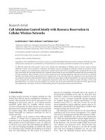
and are ordered as shown in Figure 1.IfS(x
1
, x

2
) < 0
(consistent with the example of the solid line), then the new
line to search on the next iteration is the line between x
0
and
x
2
.If0<S(x
1
, x
2
) (consistent with the example of the broken
line), then the new line to search is the line between x
1
and
x
3
.
Motivated by a desire for predictable convergence, we add
the constraint that each iteration must scale the line down by
a constant value 0 <γ<1, regardless of which interval is
chosen as the new interval. This means that
|x
2
−x
0
|=|x
3
−x

1
|=γ|x
3
−x
0
|,
(6)
|x
1
−x
0
|=|x
3
−x
0
|−|x
3
−x
1
|=

1 −γ

|
x
3
−x
0
|.
(7)

Regardless of the subjective score, the new shorter line
(between x
0
and x
2
or between x
1
and x
3
)alwaysinherits
an interior point from the longer line (x
1
in first case
and x
2
in the second case). Motivated by a desire to use
paired comparisons efficiently, we add the constraint that this
inherited (from iteration i) interior point must be one of the
two interior points evaluated in iteration i +1.
4 EURASIP Journal on Image and Video Processing
γ ·|X
3
−X
0
|
(1 −γ) ·|X
3
−X
0
|

(1 −γ) ·|X
3
−X
0
|
γ ·|X
3
−X
0
|
x
3
x
2
x
1
x
0
0
0.1
0.2
0.3
0.4
0.5
0.6
0.7
0.8
Objective function
Figure 1: Example relationships for four points in the line search.
Consider the case where the result of iteration i is the

line between x
0
and x
2
(consistent with the solid line in
the example of Figure 1). That new shorter line inherits the
interior point x
1
.Initerationi + 1 a second interior point
must be added. If this new point is inserted to the left of
x
1
,thenx
1
would now (iteration i + 1) serve the role that
x
2
played in iteration i.Using(6) we conclude that
|x
1
−x
0
|=γ
2
|x
3
−x
0
|
. (8)

Comparing (7)and(8) we conclude that
γ
2
=

1 −γ

so γ =
−
1+
√
5
2
. (9)
Finally,
1
γ
= γ +1=
1+
√
5
2
= ϕ ≈ 1.618 . (10)
If the new point is inserted to the right of x
1
,thenx
1
would now (iteration i + 1) serve the same role that it played
in iteration i.Using(6)and(7) we conclude that
|x

1
−x
0
|=

1 −γ

|
x
3
−x
0
|=

1 −γ

γ|x
3
−x
0
|, (11)
but this can only be solved by γ
= 1, which violates the
allowed range on γ. Thus the new point must be inserted to
the left of x
1
.
If iteration i produces the line between x
1
and x

3
(consis-
tent with the broken line in the example of Figure 1), an anal-
ogous set of results will follow. Thus, γ
= 1/ϕ is the only value
to use in (6)and(7) to locate x
1
and x
2
so that the uniform-
scaling-per-iteration constraint and the interior-point-reuse
constraint are satisfied. The line to search scales by γ
= 1/ϕ at
each iteration. The irrational number ϕ is called the golden
section or golden mean. It defines an aesthetically pleasing
rectangle that has been used widely in architecture and art
and also lends its name to this line search algorithm [16].
In GAST this golden section line search iterates until
S(x
1
, x
2
) = 0and|x
2
− x
1
| < Δ
t
,whereΔ
t

is a termina-
tion parameter. This condition indicates that there is no
preference between two signals whose parameterizations
are sufficiently close to each other. The algorithm returns
(1/2)(x
2
+ x
1
) as the approximation to the point on the
original line where the objective function is maximized. Our
proof-of-concept experiments indicate that the approxima-
tion is a good one. If S(x
1
, x
2
) = 0whenΔ
t
≤|x
2
−x
1
|,then
x
1
and x
2
are moved apart in increments until a nonzero vote
is returned. This is a special case that breaks from the golden
section constraints.
2.4. Entire Algorithm. To start the GAST algorithm, one must

select a starting point, x
0
,inthen-dimensional parameter
space. We have successfully used both deterministic points
on the boundary of the space and randomly selected interior
points. The direction-finding algorithm is applied to find

δ(x
0
), indicating the direction of steepest ascent from x
0
.
Next, x
0
and

δ(x
0
) are provided to the line search algorithm,
which searches in the direction

δ(x
0
)fromx
0
to the
boundary of the search space and returns the maximizing
point x
1
.

The direction-finding algorithm is then used to find

δ(x
1
), which shows the direction of steepest ascent from x
1
.
Line searching and direction finding continue to alternate
in this fashion until a terminating condition is satisfied.
At any iteration, the output of the last line search is the
best approximation to the point in the parameter space that
maximizes the objective function.
One terminating condition is

δ(x
i
) = 0, since this
indicates that there is no direction to move from x
i
to
increase the objective function. Equations (2)through(4)
show that this could be due to subjective scores of zero
(no differences detected), a local maximum, or a local
minimum that is judged to be perfectly symmetrical in
all n dimensions. Terminating in a local minimum is not
desirable; so if this is deemed a possibility, one should test
for it (the test is analogous to the one in (3)) and restart the
GAST algorithm from a new starting point as necessary. The
algorithm also terminates if the distance between the input
and output points of a line search is less than Δ

t
,sincefuture
iterations will be unlikely to move the result outside that
neighborhood.
The GAST algorithm climbs the surface of the objective
function to find a maximal value. If multiple local maxima
exist, the algorithm will find one of them but there is no
guarantee that it will be the global maximum. If multiple
local maxima are suspected, then multiple trials using
multiple starting places will help to identify them.
2.5. GAST Algorithm Implementation. The direction finding
and the golden section line search algorithms were coded
inside objects called “tunes” (since our first experiment
involved musical excerpts) such that all calculations take
place transparently to an outer algorithm that facilitates
subject interaction. The outer algorithm needs only to
instantiate said tunes by specifying x
0
, Δ
d
,andΔ
t
,request
parameter pairs associated with the signal pairs that are
EURASIP Journal on Image and Video Processing 5
presented, submit subjective scores, and keep track of all tune
objectsthatitinstantiated.
The outer algorithm is also responsible for drawing
a graphical user interface to be used by the subject, as
well as instantiating, polling, and updating necessary tune

objects, presenting signals to subjects, handling subject
votes, randomizing tune play order, and ensuring that each
search terminates. The MNRU and T-Reference algorithms
described in Section 3.1 execute rapidly; so it was possible
to generate the required audio signals just before they
were played. Likewise, the image processing described in
Section 3.2 executes very quickly and the required pairs of
images were created on demand.
For our second experiment, “tune” objects were renamed
to be “pics,” but they and the outer algorithm were otherwise
largely unchanged. Fixes for two unforeseen corner cases
were integrated, methods to store and retrieve metadata were
added, and 3D graph support was added to the plotting
code. A terminating condition was added that prevented
the algorithm from initiating a sixth-direction finding stage,
used the resting point of the fifth line search for the overall
resting place of the object, and marked the object (i.e., GAST
task) as complete. Finally, the ability to randomly reverse
parameter output order and compensate the subjective scores
for this reversal (thus randomizing stimulus presentation
order) was added to the objects, thus relieving the outer
algorithm of that responsibility.
GAST software is available at rdoc
.gov/audio/ for those who wish to experiment with the GAST
technique.
3. GAST Experiments
We have applied GAST in three different applications. Our
initial experiment was a proof-of-concept experiment using
audio reference conditions to create a simple, controlled
quality surface over a two-dimensional parameter space. The

experiment and the results are described in Section 3.1.We
later used GAST to find the optimizing values of two quan-
tization parameters in a wavelet-based image compression
scheme and full details are given in Section 3.2.
In an additional experiment, we created a modified
version of the GAST algorithm to locate quality matches,
rather than quality maxima. The application was a one-
dimensional experiment, and the goal was to identify bit-
error rates (BER) that resulted in specific reference speech
quality levels. In one-dimensional problems there is only one
line to search—no direction finding is required. Each paired
comparison involved a reference recording and a recording
from the speech coder under test at the BER under test. The
result of the comparison would cause the BER to be increased
or decreased accordingly (a line search) until the point of
equivalence was found.
Each of the three experiments has affirmed the utility and
efficacy of the GAST algorithm.
3.1. Audio Quality GAST. As an initial test of the GAST
concept, we devised an audio experiment using two ref-
erence conditions that simulate audio coding. The use of
two reference conditions (instead of two actual coding or
transmission system parameters) allowed us to create a
two-dimensional parameter space with a known region of
maximal audio quality.
3.1.1. Audio Quality Parameter Space. Audio signals were
passed through the two reference conditions in sequence to
generate a controlled, known quality surface over a two-
dimensional parameter space. The first reference condition
was the modulated noise reference unit (MNRU) [17]. This

condition adds signal-correlated Gaussian noise to the audio
signal at the specified SNR of Q dB:
y
k
= x
k
+ x
k
·n
k
·10
−Q/20
= x
k
·

1+n
k
·10
−Q/20

, (12)
where x
k
, y
k
,andn
k
are input, output, and unit-variance
zero-mean Gaussian noise samples, respectively. The noise

added by the MNRU sounds like that produced by some
waveform coders.
The second reference condition was modeled after the
T-Reference described in [18, 19]. The T-Reference imparts
a controlled level of audio distortion through short-term
time warping. This distortion can be described as “warbling”
or “burbling” and is similar to that produced by some
parametric coders.
The T-Reference operates on frames of 256 audio samples
(5.8 milliseconds). In each group of three sequential frames,
the first is temporally compressed, the second is untouched,
and the third is temporally stretched.
More specifically, with frames labeled 1 through N,
the T-Reference applies temporal compression to frames
numbered 1 + 3
· k, it does not change frames numbered
2+3
· k, and it applies temporal expansion to frames
numbered 3 + 3
· k, k = 0,1,2, Temporal compression
is accomplished by deleting every Tth sample, and the
complementary temporal expansion is accomplished by
interpolating a sample between every Tth and T+1st sample.
Since
256/T samples are deleted from the first frame in the
group and the same number of samples are interpolated into
the third frame in the group, the total number of samples in
each group of three frames is preserved at 3
·256.
The unit-less parameter T can be set to any integer in the

range from 2 to 256. Larger values of T correspond to less
distortion.
We developed GAST software to work in a normalized
[0, 1] parameter space. Thus, we mapped this range to Q and
T values according to
Q
=−85 · p
2
1
+ 100 · p
1
,
T
= 1+

2
(−15·p
2
2
+13·p
2
+2)

,
(13)
where [
·] denotes rounding to the nearest integer. These
relationships are displayed in Figure 2. They were selected to
smoothly traverse a wide range of Q and T values and have
different shapes, asymmetric slopes, and a single interior

maximum for both Q and T.
From Figure 2 we can conclude that in the two-
dimensional space (p
1
, p
2
), there is a line segment of
6 EURASIP Journal on Image and Video Processing
10.90.80.70.60.50.40.30.20.10
p
1
or p
2
0
5
10
15
20
25
30
Q(p
1
)(dB)orT(p
2
)
Figure 2: Q as a function of p
1
(dashed), and T as a function of p
2
(solid).

10.90.80.70.60.50.40.30.20.10
p
1
(Q)
0
0.1
0.2
0.3
0.4
0.5
0.6
0.7
0.8
0.9
1
p
2
(T)
6. Line to search
5. Direction finding
Tr u e m a x im u m
7. End of line search
4. End of line search
2. Direction finding
3. Line to search
1. Starting point
Figure 3: Example trajectory of an audio experiment GAST trial;
details are in text.
numerically maximal audio quality extending from the point
(0.60,0.39) to the point (0.60,0.48). This segment is shown

as a solid vertical line in Figures 3 and 4. The reference
condition parameter values associated with this region of
maximal audio quality are Q
= 29.4dBandT = 29.
3.1.2. Audio Quality Protocol. This audio GAST experiment
used eight five-second musical segments covering a range of
instruments and musical styles. These were excerpted from
compact discs and the native sample rate of 44,100 samples
per second was maintained through the experiment.
A PC testing protocol was used. Two audio signals were
presented sequentially and five possible subjective responses
were allowed: “The audio quality of the second recording
10.90.80.70.60.50.40.30.20.10
p
1
(Q)
0
0.1
0.2
0.3
0.4
0.5
0.6
0.7
0.8
0.9
1
p
2
(T)

Figure 4: Start and end points for 35 audio experiment GAST trials
shown with black squares and blue circles, respectively. The light
blue ellipse shows the mean and 95-percent confidence interval for
all end points. The bold orange vertical line represents region of
numerically maximal audio quality.
is much better than, better than, the same as, worse than,
or much worse than, the first recording.” The associated
subjective scores are 2, 1, 0,
−1, and −2, respectively. After the
presentation of each pair of signals, a subject could submit a
vote or request to hear the pair played again.
Subjects were seated in a sound isolated room with
background noise measured below 20dBA SPL. Audio
signals were presented through studio-quality headphones at
the individually preferred listening level. A PDA was used to
present the prompts and collect the votes.
Six subjects participated in the experiment. Each ran the
GAST algorithm on four of the eight musical selections,
using two different starting places per selection. One starting
place was the origin of the parameter space; the other was
randomly chosen for each musical selection and each subject.
Thus, each subject started eight different GAST tasks, and in
each trial the subject made one step of progress on one task
randomly selected from the eight. We used the direction-
finding step size Δ
d
= 0.15 and the terminating condition
Δ
t
= 0.20.

3.1.3. Audio Quality Results. In this initial GAST experiment,
some tasks ended prematurely due to implementation issues,
subject time limitations, and lack of a quality gradient near
the corners of the parameter space. Excluding these special
cases, the GAST algorithm consistently located a point of
maximal perceived quality and then terminated as expected.
Figure 3 shows an example GAST task trajectory. The
region of numerically maximal audio quality is shown
with a bold orange vertical line. The square at the origin
indicates the starting location. The triangles connected
EURASIP Journal on Image and Video Processing 7
to that square indicate the two points used in the first
direction-finding step. The audio signal parameterized by
the triangle at (0.15,0) was voted “much better” than the
signal associated with the origin; so S((0, 0)
T
,(0.15, 0)
T
) =
2, where (·)
T
indicates the transpose operator. Similarly,
S((0, 0)
T
,(0,0.15)
T
) = 1.
These two scores yielded the normalized direction vector

δ(x) = (1/

√
5)·(2, 1)
T
and this led to a search of the line that
runs up and to the right. Points played on this line are shown
with diamonds, and the result of the line search is shown
with a circle. The four points connected to that circle were
played as part of the second direction-finding step. This led
to a search of the line that runs toward the upper left corner
of the figure. Again, points played are shown with diamonds,
and the final result is shown with a circle. This result is very
close to the location of numerically maximum audio quality.
This task required 13 votes.
Different musical selections can reveal or mask dis-
tortions in different ways, and these distortions may be
perceived differently by individual subjects. Thus, perceived
quality is a function of signals and subjects as well as the
device under test. Averaging results over a representative
sample of relevant signals and subjects gives the most
meaningful perceived quality results.
Figure 4 shows the GAST algorithm start (black squares)
and end (blue circles) points for the 35 audio experiment
GAST tasks that ran to completion. An average of 15.6 votes
was required per task. The end points cluster around the
line segment of numerically maximal audio quality (the bold
orange vertical line), as expected. The mean and 95-percent
confidence intervals for the p
1
and p
2

dimensions are shown
with a light blue ellipse. For the 35 combinations of subjects
and musical selections, we are 95 percent confident that the
mean location of maximal perceived audio quality is between
0.571 and 0.649 in p
1
dimension (29.1 ≤ Q ≤ 29.4dB),and
between 0.404 and 0.436 in the p
2
dimension (T = 29). This
result is consistent with the known location of numerically
maximal audio quality and required 15.6
× 35 = 546 PC
presentations (not including any replays) and 546 votes.
To locate this point with the same resolution using
ES ACR testing, one would need about 13 samples
((0.649
−0.571)
−1
= 12.8) in the p
1
dimension and 32
samples ((0.436
−0.404)
−1
= 31.3) in the P
2
dimension,
resulting in a 416-sample grid on the parameter space.
Evaluating each point with all 35 combinations of musical

selections and subjects would require 416
×35 = 14, 560 ACR
presentations (not including any replays) and votes. This is a
lower bound. If 35 trials per point in the parameter space
do not result in statistically significant differences between
adjacent parameter space samples in the neighborhood of the
quality maximum, then additional trials would be required
to locate the maximum with a resolution that matches GAST.
Thus, we find that the number of votes required is reduced by
at least a factor of 14, 560/546
= 26.7.
Figure 5 shows the average convergence of the 35 GAST
trials. Seventeen trials started at the origin and eighteen
started at random locations. The resulting average Euclidean
distance between starting places and the nearest point in the
θ = 1
θ
= 2
θ
= 5
43210
GAST iterations
0
0.1
0.2
0.3
0.4
0.5
0.6
Mean distance from optimal region

Figure 5: Average convergence performance for human subjects
and Monte Carlo simulations for a parametrized family of “perfect
subjects.”
region of maximal audio quality is 0.54. With each iteration
of the GAST algorithm this average distance decreases and an
asymptotic value of 0.1 is approached after two iterations.
Figure 5 also shows the results of three Monte Carlo
simulations. In these simulations, software emulated a family
of “perfect subjects.” These hypothetical subjects could
decompose the audio signals and independently measure the
levels of impairment due to MNRU and T-Reference relative
to the best audio quality in the experiment (Q
max
= 29.4and
T
max
= 29):
ζ
i
=

(
Q
i
−Q
max
)
2
+


1
2
(
T
i
−T
max
)

2
. (14)
The index i
= 1, 2 indicates internal measurements for
the first and second audio recordings heard, respectively.
Changes in T are harder to detect than changes in Q and the
factor of 1/2in(14) provides a very rough match between the
two scales.
The “perfect subjects” then voted with perfect consis-
tency but finite sensitivity (θ) according to
(
ζ
1
−ζ
2
)
≤−2θ =⇒ S =−2
(
much worse
)
,

−2θ<
(
ζ
1
−ζ
2
)
≤−θ =⇒ S =−1
(
worse
)
,
−θ<
(
ζ
1
−ζ
2
)
<θ
=⇒ S = 0
(
same
)
,
θ
≤
(
ζ
1

−ζ
2
)
< 2θ
=⇒ S = 1
(
better
)
,
2θ
≤
(
ζ
1
−ζ
2
)
=⇒ S = 2
(
much better
)
.
(15)
For each simulation 16,000 tasks with random starting places
were used. This produced an average initial distance of 0.37.
As expected, smaller values of θ result in quicker
convergence to lower asymptotic distance values. The setting
θ
= 5 gives an average convergence curve similar to that
of our human subjects, excepting the fact that the average

starting distances are different. This corresponds to a baseline
8 EURASIP Journal on Image and Video Processing
MNRU sensitivity of Q
= 5dB and a baseline T-Reference
sensitivity of 10 T units.
3.2. Image Quality GA ST. We were invited to contribute our
work on the GAST algorithm to this special issue of this
journal. This motivated us to apply the GAST algorithm to
image quality assessment to demonstrate its applicability in
that domain.
A typical problem in image coding is rate minimization:
minimize the number of bits used to encode an image
while holding the image quality at or above some target
level (e.g., transparent coding). The dual to this problem is
the quality maximization problem: maximize image quality
while holding the bit-rate at some constant value. This
problem fits well with GAST and is the subject of the
experiment.
3.2.1. Image Quality Parameter Space. There are many image
coding frameworks that one could invoke for this experiment
and we elected to use the JPEG 2000 framework [20–
22]. JPEG 2000 is generally considered an advance over
the original DCT-based JPEG standard [23]intermsof
rate-distortion performance, and this advance comes with
additional cost in terms of computational complexity. JPEG
2000 offers lossy-to-lossless progressive coding, scalable
resolution, region of interest features, and random access.
JPEG 2000 is used in digital cinema, fingerprint databases,
remote sensing applications, and medical imaging [22]. We
recognize JPEG 2000 as a mature, successful, and highly

optimized coding technique. As such, it also provides a
natural basis for further investigations in image coding.
Lossy JPEG 2000 compression transforms level-shifted
YUV pixel values with the Daubechies 9/7 discrete wavelet
transform (DWT). The key to minimizing rate or maximiz-
ing quality in JPEG 2000 lies in the quantization and encod-
ing of the resulting DWT coefficients. In typical operation,
the quantization step-size is made much smaller than would
be ultimately necessary—“overquantization” is performed.
This is followed by a multipass bit-plane significance coding
algorithm with lossless entropy coding that uses an adaptive
arithmetic coding strategy. The quantization and coding
stages are tied together through a sophisticated rate-control
algorithm that seeks to reduce mean-squared error (MSE) or
visually weighted MSE as much as possible as it assigns the
available bits.
Quantization of DWT coefficients in the context of
JPEG 2000 has been studied extensively. The basis func-
tions of the DWT decomposition from different levels and
orientations have differing visual importances. Quantization
noise imposed on the associated coefficients produces visual
distortions that are localized in spatial frequency and
orientation and can also be correlated to the image. Thus,
quantization noise on different DWT coefficients will have
differing levels of visibility.
The pioneering experiments in [24] found visibility
thresholds for each of the various levels and orientations
of the wavelet basis functions. These thresholds translate
to step-sizes for uniform quantizers—following these step
sizes would keep DWT quantization noise for each individual

DWT basis function below the visible threshold.
Numerous additional empirical studies and theoretical
derivations have treated the topics of contrast sensitivity
functions, visual summation of quantization errors, self-
masking, neighborhood masking, and others. (These often
jointly address the intrinsically linked issues of quantization
and rate control.) Individual examples can be found in [25–
28] and more comprehensive overviews can be found in
[22, 29]. Much of this work has been incorporated (perhaps
implicitly) into JPEG 2000, Part 1, and (more explicitly) into
Part 2.
Our GAST experiment also treats the quantization
of DWT coeffi
cients. Instead of overquantizing and then
seeking rate reduction in a coding stage, we use GAST to
drive the design of rate-constrained, nonuniform quantizers
with arbitrary dead-zones that maximize image quality.
Clearly, this is not a proposal for a practical image coding
implementation. Instead, it is an experimental investigation
of nonuniform quantization and arbitrary dead-zones in the
context of DWT coefficients. This investigation is driven by
true human visual perception (not MSE, SNR, or a visually
based computed distortion metric). To our knowledge, both
the optimization problem and the optimization technique
that we describe below are unique.
We apply the Daubechies 9/7DWT to each color plane
of a 512
× 512 pixel image with 8 bits/pixel, successively
decomposing it to four levels. (Four levels are sufficient to
capture most of the available DWT benefit in this context.)

At the fourth level the coefficients of each orientation (LL,
LH, HL, and HH) form a 32
× 32 block (32 = 512 × 2
−4
).
Coefficients from the LH and HL orientations follow the
same Laplacian distribution:
f
c
(
c
)
=
1
√
2σ
e
−|c|(
√
2/σ)
(16)
so they can share the same quantizer design.
We use GAST to optimize two design parameters for
a single quantizer for the fourth-level, Y-plane coefficients
from the LH and HL orientations. These are the only coeffi-
cients we quantized before application of the inverse DWT to
reconstruct the image. The majority of the energy (and thus
the majority of the coding problem) lies in the coefficients of
the final, fourth level. Additional similar experiments could
be designed to further investigate quantization of coefficients

from the LL orientation (typically modeled by the General-
ized Gaussian distribution or the uniform distribution), the
HH orientation (modeled by Laplacian distribution but with
lower variance than LH/HL coefficients), or coefficients from
lower levels of the decomposition (Laplacian but with lower
variance than coefficients from the fourth level).
A histogram (taken across 43 images) confirms that
the distribution of the fourth-level, Y-plane, LH/HL DWT
coefficients approximately matches that of the zero-mean
Laplacian random variable. To allow finite quantization, we
limit the coefficient magnitudes to 1200 (limiting occurs for
about 0.01% of the coefficients). For ease of presentation
here, and without loss of generality, we scale the limited
DWT coefficients to the range [
−1, 1].
EURASIP Journal on Image and Video Processing 9
Next we define the quantizer Q(c, Δ
dz
, α,N)thatoperates
on the DWT coefficient c:
|c|≤Δ
dz
=⇒ Q
(
c, Δ
dz
, α,N
)
= 0,
Δ

dz
< |c|=⇒Q
(
c, Δ
dz
, α,N
)
= sign
(
c
)

NF
α

|
c|−Δ
dz
1 −Δ
dz

,
(17)
where the compander function F
α
(·)isdefined:
α
= 0 =⇒ F
α
(

x
)
= x,
α
/
=0 =⇒ F
α
(
x
)
=
1 −e
−αx
1 −e
−α
.
(18)
The quantizer dead-zone is defined by Δ
dz
,0 < Δ
dz
< 1.
The dead-zone extends from
−Δ
dz
to +Δ
dz
,sothedead-
zone width is 2Δ
dz

,andcoefficient values in this range are
reconstructed as zero. In addition to this central cell, the
quantizer has N cells to cover the remaining negative range
and N cells to cover the remaining positive range (N
=
1, 2,3, ). Thus the quantizer has 2N + 1 quantization cells
total and it maps real numbers in the interval [
−1, 1] to the
integers
{−N, −(N − 1), ,N − 1, N}.
In addition, the quantizer shape (the local quantizer
cell width relationship) is controlled by α (
−∞ <α<
+
∞) through the compander function F
α
(·). This function
maps the range [
−1, 1] onto itself. When α = 0, F
α
(·)is
linear and the resulting quantizer has uniform cell widths
(with the possible exception of the central, dead-zone cell).
If 0 <α, the resulting quantizer has cell widths that
increase as one moves away from the origin. Increasing α
strengthens the effect. When α<0, quantizer cell widths
decrease as one moves away from the origin and the effect
is strengthened by decreasing α.Examplesofthequantizer
input-output relationship defined by (17)and(18)are
shown in Figure 6.Equations(17)and(18)emphasizethat

nonuniform quantizers can be implemented by a nonlinear
function followed by a uniform quantizer.
An approximation,
c, to the original coefficient value, c,
can be recovered by the inverse quantizer:
Q
(
c
)
= 0 =⇒ c = 0,
Q
(
c
)
/
=0 =⇒ c
= sign
(
Q
(
c
))

(
1
−Δ
dz
)
G
α


|
Q
(
c
)
|−0.5
N

+ Δ
dz

,
(19)
where the compander function G
α
(·) is introduced in order
to exactly invert the operation of F
α
(·):
α
= 0 =⇒ G
α
(
x
)
= x,
α
/
=0 =⇒ G

α
(
x
)
=
−
ln
(
1 −x
(
1 −e
−α
))
α
.
(20)
The resulting mean-squared quantization error is

2
=
E((c − c)
2
) and this can be minimized by using a pdf-
optimized quantizer design. An approximate design criterion
α = 4
α
= 2
α
= 0
α

=−2
10.90.80.70.60.50.40.30.20.10
Input, c
0
1
2
3
4
5
6
7
8
9
Output, Q(c)
Figure 6: Example quantizer function for positive inputs, α =
−
2, 0,2, and 4, Δ
dz
= 0.1, and N = 9. (Small vertical offsets have
been added for clarity.)
is that the quantizer cell widths w(c) are proportional
to f
−1/3
c
(c)where f
c
(·) is the pdf for the coefficients to
be quantized (see e.g., [30]or[31]). Under this design
criterion, areas with lower probability densities are assigned
wider quantization cells. This design criterion becomes exact

(minimizing

2
) in the high-rate (large N) limit. For the
Laplace pdf (16), the f
−1/3
c
rule dictates the cell width
relationship:
w
(
c
)
∼ e
|c|(
√
2/3σ)
. (21)
The local quantizer cell widths defined in (17)and
(18) are driven by the reciprocal of the local slope of the
compander function F
α
(·):

∂
∂c
F
α
(
c

)

−1
=
(
1
−e
−α
)
e
cα
α
, (22)
resulting in the cell width relationship:
w
(
c
)
∼ e
|c|α
. (23)
Comparison of (21)with(23) reveals that the choice
α
= α
0
=
√
2
3σ
(24)

will give the Laplace pdf-optimized shape to the quantizer
defined in (17)-(18). In (24) σ is the standard deviation of
the DWT coefficients after scaling to the range [
−1, 1].
Thus (17)and(18) define a quantizer parametrized by
dead-zone (Δ
dz
), shape (α), and size (N). Together these
three parameters determine the rate and the distortion of
the quantizer. Because dead-zone and shape interact in
determination of both rate and distortion, they must be
optimized jointly. We use the GAST algorithm to find jointly
optimal values of Δ
dz
and α forafixedquantizerbitrate.And
the optimization is with respect to perceived image quality
10 EURASIP Journal on Image and Video Processing
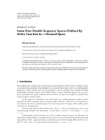
(a) (b) (c)
(d) (e)
Figure 7: The five images used in the image quality experiment. Original images with dimensions larger than 512 × 512 were cropped as
shown.
rather than mean-squared error or some visually weighted
variant of mean-squared error.
By convention, GAST parameters range from 0 to 1.
Preliminary visual inspection motivated us to apply the
mapping
p
1
= 12Δ
dz

(25)
to search Δ
dz
values from 0 up to 1/12 (DWT coefficients
normalized to [
−1, 1]). Similarly
p
2
= 0.5+0.5
α
1.5α
0
(26)
allows a search of α values from
−1.5α
0
to 1.5α
0
.Underthis
mapping p
2
= 0.5 gives the uniform quantizer, and p
2
=
5/6 ≈ 0.83 gives the pdf-optimized quantizer of (24). For
any pair (p
1
, p
2
) the GAST software calculates and applies

the corresponding values of Δ
dz
and α as given in (25)and
(26). This is done for N
= 1,2, 3 ··· until the entropy of
the quantized coefficients approximately matches the target
quantizer bit rate.
The target rates are 1.5 or 2.0 bits/coefficient. One of
these values was selected for each image in the experiment
after preliminary visual inspections. The goal of this manual
rate-selection process was to ensure an image quality gradi-
ent on the parameter space for each image rather than image
quality that is saturated at “very bad” or “very good” due to
images that are hard to code or easy to code (or equivalently
a target rate that is too low or too high).
Part 1 of JPEG 2000 standard specifies a uniform scalar
quantizer (α
= 0, and quantizer cell width is Δ
q
)andadead-
zone that is twice as wide as the other quantizer cells (Δ
dz
=
Δ
q
). Part 2 allows for arbitrary dead-zone widths, but this can
interfere with the intrinsic embedding property that follows
from the constraint Δ
dz
= Δ

q
.
The work of [22] reports that rate-distortion optimized
dead-zone widths follow (1/2)Δ
q
< Δ
dz
< Δ
q
.Theworkof
[32] suggests the value Δ
dz
≈ (3/4)Δ
q
.And[33]proposes
Δ
dz
∼ 1/C
95
where C
95
is the 95th percentile point of the
coefficient distribution.
These quantizers are special cases of the more general
quantizer described by (17)and(18). In Section 3.2.3 we
compare three of these with the visually optimal quantizer
designs identified by GAST.
3.2.2. Image Quality Protocol. Five 512
× 512 images were
used in the test. These were provided by other image

processing labs and were in some cases cropped to obtain this
size. Thumbnails of the images can be seen in Figure 7.
In each trial two versions of an image (corresponding to
quantization based on two points in the parameter space)
EURASIP Journal on Image and Video Processing 11
were presented side-by-side on an LCD touch-screen. The
prompt “Which image has higher quality?” appeared at the
top of the screen, and subjects could select either image by
touching the button below it, or they could touch a button
labeled “No Quality Difference.” This produced scores of
±1
to indicate an image preference, and 0 for no preference.
A 150 cm by 75 cm table was placed in the center of a
sound-isolated room. A 54.5 cm color touchscreen monitor
was placed 14 cm from and bisecting the long edge of the
table nearest the room’s entrance. The monitor has a pixel
density of approximately 40 pixels per centimeter (1920
×
1080 pixels, 47.5 cm by 27 cm). A comfortable chair was
placed near the monitor.
The lighting level was controlled by a dimmer. In order to
comply with the lighting levels specified in [3], the viewing
distance must be known. Viewers were given the freedom to
choose their viewing distance; so a lookup table was created.
The lookup table included ranges from 27.5 to 67.5cm (or
1100 to 2700 pixels) in increments of 5 cm (200 pixels). A
digital lux meter was used to measure the illuminance of
the monitor and the wall behind the monitor at a given
distance. These readings iteratively served as a guide to
correct the position of the dimmer for each viewing distance.

These dimmer positions were recorded and linked to viewing
distance in the lookup table.
Viewers were instructed to adjust the chair’s distance
from the monitor; so they could comfortably compare
detailed images. After viewers selected a comfortable posi-
tion, the approximate viewing distance was measured and
the lookup table was consulted to find the proper dimmer
setting.
Two of the room’s four adjustable lights were positioned
such that a semiuniform field of light illuminated the gray
background wall. The other two lights were pointed towards
the side walls. Very little light ended up on the wall behind
the subject, thus minimizing reflections on the surface of the
monitor.
Color calibration hardware and software was used to
optimize the monitor’s color profile for accuracy and optimal
contrast given the room’s lighting environment.
Twenty subjects participated in the experiment. Subjects
wore any vision correction that they normally would for
screen-based work at their preferred viewing distance. Each
subject ran the GAST algorithm on all five images, using two
randomly selected starting locations in the parameter space
for each image. Thus, each subject performed ten GAST
tasks, and in each trial the subject made one step of progress
on one task randomly selected from the ten. A total of 199
GAST trials were completed. This falls short of 20
×10 = 200
due to time limitations for one subject. Subjects typically
spent around 35 minutes in the test. We used the direction-
finding step size Δ

d
= 0.20 and the terminating condition
Δ
t
= 0.15.
3.2.3. Image Quality Results. Figure 8 shows the starting
and ending points for the 199 completed GAST trials. The
starting points are randomly distributed across the search
space, and the ending points are mostly clustered near the
center of the search space. Some ending points remain close
10.90.80.70.60.50.40.30.20.10
p
1
(quantizer dead-zone size)
0
0.1
0.2
0.3
0.4
0.5
0.6
0.7
0.8
0.9
1
p
2
(quantizer shape)
Figure 8: Starting and ending points for all 199 completed image
GAST tasks shown by black squares and blue circles, respectively.

The gray tick marks in the axes indicate the p
1
or p
2
value of each
starting point.
Table 1: Means and 95% Confidence Interval Values of p
1
and p
2
for each Image.
Image Mean 95% c.i.
p
1
p
2
p
1
p
2
a 0.599 0.430 0.060 0.086
b 0.588 0.519 0.073 0.064
c 0.631 0.413 0.046 0.082
d 0.636 0.469 0.048 0.079
e 0.576 0.423 0.073 0.071
all 0.606 0.451 0.027 0.034
to or identical to their starting points. This indicates a lack
of local quality gradient. Indeed, in the corners of the search
space, the image quality is consistently low—there is no local
quality gradient. In addition, some random starting places

happen to fall near the point of maximum image quality and
those trials end quickly.
Figure 9 shows the ending points for the 199 trials coded
by image and Figure 10 shows the mean ending point for
each image with a cross. The major and minor axes of the
ellipse drawn about each cross indicate the 95% confidence
interval for that mean location. While some per-image
differences are observable in these results, they are not large,
especially in light of the confidence intervals. Ta b l e 1 shows
the numerical results for each image.
Figure 11 shows the grand mean result and 95% confi-
dence intervals for image GAST experiments taken over the
five images. In addition, the mean (across the five images)
locations of three different reference quantizers described in
Section 3.2.1 are displayed. These quantizers all use uniform
12 EURASIP Journal on Image and Video Processing
10.90.80.70.60.50.40.30.20.10
p
1
(quantizer dead-zone size)
0
0.1
0.2
0.3
0.4
0.5
0.6
0.7
0.8
0.9

1
p
2
(quantizer shape)
Figure 9: Ending points for all completed image GAST tasks. Red
dots correlate with image a, gray with image b, blue with image c,
green with image d, and orange with image e. The gray tick marks
in the axes indicate the p
1
or p
2
value of each ending point.
10.90.80.70.60.50.40.30.20.10
p
1
(quantizer dead-zone size)
0
0.1
0.2
0.3
0.4
0.5
0.6
0.7
0.8
0.9
1
p
2
(quantizer shape)

Figure 10: Mean and 95% confidence intervals for all completed
image GAST tasks, separated by image. Similarly to Figure 9,thered
ellipse correlates with image A, gray with image B, blue with image
C, green with image D, and orange with image E.
quantization bins p
2
= 0.5(α = 0.0) with the possible
exception of the central bin defined by the dead-zone. Thus,
they differ only with respect to p
1
which controls Δ
dz
.These
quantizers are (from left to right) the uniform rounding
quantizer (Δ
dz
= 1/2Δ
q
), the quantizer proposed in [32]
(Δ
dz
= (3/4)Δ
q
), and the JPEG 2000 Part 1 quantizer
Part 1MarcURQ
0.70.60.50.40.3
p
1
(quantizer dead-zone size)
0.4

0.5
0.6
p
2
(quantizer shape)
Figure 11: Mean and 95% confidence intervals for all completed
image GAST tasks. Compare with three labeled quantizer designs,
left to right: Uniform Rounding Quantizer (URQ), Quantizer of
[32] (Marc), JPEG 2000, Part 1 Quantizer (Part 1).
(Δ
dz
= Δ
q
). Of these three options, the GAST results are
closest to the JPEG 2000 Part 1 quantizer, though in context
of this particular experiment, a slightly larger dead-zone
(p
1
= 0.61, Δ
dz
= 0.051) may be desirable.
Next, we consider the quantizer shape parameter α which
is controlled by P
2
. To minimize MSE, one would select a
pdf-optimized quantizer, α
= α
0
and p
2

= 5/6. This is
a compressive function and quantizer bins get larger as one
moves away from zero. Consideration of visual self-masking
suggests the function, H(x)
= x
0.7
[29]. While not directly
comparable with (18), this is also a compressive function and
thus would correspond to 0 <αand 0.5 <p
2
.ButtheGAST
results say that image quality is maximized, on average, by
p
2
= 0.45, corresponding to a slightly negative shape factor
(α
=−0.15α
0
)andaslightlyexpansive function, with bins
getting slightly smaller as one moves away from zero.
This quantizer shape result is barely statistically signifi-
cantly different from p
2
= 0.5andα = 0.0, which would
point to uniform quantization as the optimal strategy, and
that may be the safest conclusion to draw. Suffice it to say that
this experiment does not suggest the use of a compressive
nonlinearity to improve image quality.
The experiment results can be summarized as follows.
When the quantizer defined by (17)-(18) is applied to the

Y-plane, level 4, LH/HL orientation, Daubechies 9/7 DWT
coefficients from the five images shown in Figure 7,thedead-
zone size and quantizer shape that maximize mean perceived
image quality are very close to the dead-zone and shape used
in JPEG 2000, Part 1. From an image coding perspective,
we may have simply reinvented the wheel. Or we could
argue that we have added additional, and unique, support
for the JPEG 2000 Part 1 quantizer design. But from the
image quality assessment perspective, we argue that we have
demonstrated a new subjective image quality maximization
technique that has surveyed a two-dimensional image coding
space and efficiently arrived at what is arguably the “right
answer.”
4. Discussion and Observations
We have presented the motivation for and development of
GAST. And we have demonstrated this novel and efficient
EURASIP Journal on Image and Video Processing 13
subjective testing technique in two different domains: audio
quality testing and image quality testing.
In the audio experiment we created a simple con-
trolled, two-dimensional parameter space using reference
conditions. Because of the already established monotonic
relationships between Q and perceived audio quality, and
between T and perceived audio quality, the region of highest
audio quality (the “right answer”) was known. This is a
necessary condition for the evaluation of a new measurement
technique. The GAST algorithm identified the right answer
accurately and efficiently. Compared with the hypothetical
comparable ES ACR subjective test, the number of votes was
reduced by at least a factor of 27, and one would expect these

savings to increase in higher-dimensional problems.
In the image experiment we optimized the dead-zone size
and shape of a quantizer for one class of JPEG 2000 DWT
coefficients. Here the “right answer” was not known—this
is a natural next step for testing a measurement technique.
GAST identified a dead-zone size and quantizer shape that
maximize image quality and these are quite close to those
defined in JPEG 2000, Part 1. We consider this to be a very
plausible “right answer.”
We emphasize again that a successful GAST task identifies
a local quality maximum. As with all such search algorithms,
there is no guarantee that this local maximum is the global
maximum. And as with all such search algorithms, there is
a battery of techniques to mitigate this potential problem.
Our work here demonstrates one of the simplest of these
techniques, the use of multiple random starting points.
When the vast majority of searches starting from across the
searchspaceendupinthesameregion,onecanhavegood
confidence that the region is preferred in the global and local
sense.
Note that GAST can be used with na
¨
ıve or expert
subjects. Expert subjects might benefit from additional
information as the test progresses. Since the end point of
each line search is the current approximation to the point of
maximal quality, experts might advantageously use feedback
on search progress to use their time even more efficiently.
For example, the message “You have just completed the nth
line search for this task” indicates that one has obtained an

approximate solution and could end the task despite the fact
that a terminating condition has not been met.
Note also that if identifying points of minimal quality
is of interest (worse case analyses), one can simply multiply
all votes by
−1 and the GAST algorithm will locate minima
instead of maxima.
The work presented here is a fairly straightforward
melding of paired-comparison subjective testing and a rather
basic search algorithm. There are many potential paths
to improve GAST performance, efficiency, and robustness.
One might undertake refinement of the terminating con-
ditions, possibly making them adaptive. Line lengths could
become adaptive; thus one would search shorter lines as the
algorithm progresses, since the start of the line should be
getting closer to the sought-after point of maximal quality.
The direction finding step size Δ
d
might be advantageously
adapted as the algorithm progresses (larger early on or when,
in flatter regions, smaller later or in steeper regions). Finally,
other search algorithms could be employed in a similar
fashion.
Acknowledgments
This work was supported by the National Telecommunica-
tions and Information Administration’s Institute for Tele-
communication Sciences. The authors would like to thank
Frank Sanders for his managerial support and the many
anonymous test subjects who participated in the subjective
experiments.

References
[1] ITU-T Recommendation P.800, “Methods for subjective deter-
mination of transmission quality,” Geneva, 1996.
[2] ITU-R Recommendation BS.1284, “General methods for the
subjective assessment of sound quality,” Geneva, 2003.
[3] ITU-R Recommendation BT.500-12, “Methodology for the
subjective assessment of the quality of television pictures,”
Geneva, 2009.
[4] ITU-T Recommendation P.911, “Subjective audiovisual qual-
ity assessment methods for multimedia applications,” Geneva,
1998.
[5]S.Tourancheau,F.Autrusseau,Z.M.P.Sazzad,andY.
Horita, “Impact of subjective dataset on the performance
of image quality metrics,” in Proceedings of the 15th IEEE
International Conference on Image Processing (ICIP ’08),pp.
365–368, October 2008.
[6] S. Voran, “Estimation of speech intelligibility and quality,” in
Handbook of Signal Processing in Acoustics,D.Havelock,S.
Kuwano, and M. Vorl
¨
aander, Eds., vol. 2, chapter 28, pp. 483–
520, Springer, New York, NY, USA, 2008.
[7] K. Seshadrinathan, R. Soundararajan, A. C. Bovik, and
L. K. Cormack, “Study of subjective and objective quality
assessment of video,” IEEE Transactions on Image Processing,
vol. 19, no. 6, pp. 1427–1441, 2010.
[8]M.H.PinsonandS.Wolf,“Anewstandardizedmethodfor
objectively measuring video quality,” IEEE Transactions on
Broadcasting, vol. 50, no. 3, pp. 312–322, 2004.
[9] S. Voran and A. Catellier, “Gradient ascent paired-comparison

subjective quality testing,” in Proceedings of the International
Wor kshop on Quality of Multimedia Experience (QoMEx ’09),
pp. 133–138, San Diego, Calif, USA, July 2009.
[10] I. E. G. Richardson and C. S. Kannangara, “Fast subjective
video quality measurement with user feedback,” Electronics
Letters, vol. 40, no. 13, pp. 799–801, 2004.
[11] U. Reiter and J. Korhonen, “Comparing apples and oranges:
subjective quality assessment of streamed video with different
types of distortion,” in Proceedings of the International Work-
shop on Quality of Multimedia Experience (QoMEx ’09),pp.
127–132, San Diego, Calif, USA, July 2009.
[12]A.B.WatsonandD.G.Pelli,“QUEST:aBayesianadaptive
psychometric method,” Perception and Psychophysics, vol. 33,
no. 2, pp. 113–120, 1983.
[13] A. Ravindran, K. M. Ragsdell, and G. V. Reklaitis, Engineering
Optimization: Methods and Applications, Wiley, Hoboken, NJ,
USA, 2nd edition, 2006.
[14] J. Nocedal and S. Wright, Numerical Optimization,Springer,
New York, NY, USA, 2nd edition, 2006.
[15] S. Boyd, Convex Optimization, Cambridge University Press,
Cambridge, UK, 2004.
14 EURASIP Journal on Image and Video Processing
[16] B. Gottfried and J. Weisman, Introduction to optimization
theory, Prentice Hall, Englewood Cliffs, NJ, USA, 1973.
[17] ITU-T Recommendation P.810, “Modulated noise reference
unit (MNRU),” Geneva, 1996.
[18] B. Cotton, “New reference condition for very low bit rate
voice coder evaluation,” CCITT SGXII Contribution D.108,
September 1991.
[19] S. Voran, “Observations on the t-reference condition for

speech coder evaluation,” CCITT SGXII Contribution SQ-
13.92, February 1992, />[20] ISO/IEC 15444-1, ITU-T T.800, “Information Technology—
JPEG 2000 image coding system,” Geneva, 2004.
[21] ISO/IEC 15444-2, ITU-T T.801, “Information Technology—
JPEG 2000 image coding system: extensions,” Geneva, 2004.
[22] P. Schelkens, A. A. Skodras, and T. Ebrahimi, Eds., The JPEG
2000 Suite, Wiley, Chichester, UK, 2009.
[23] ISO/IEC IS 10918-1, ITU-T T.81, “Information Technology—
Digital compression and coding of continuous-tone still
images—part 1: Requirements and guidelines,” Geneva, 1993.
[24] A. B. Watson, G. Y. Yang, J. A. Solomon, and J. Villasenor,
“Visibility of wavelet quantization noise,” IEEE Transactions on
Image Processing, vol. 6, no. 8, pp. 1164–1175, 1997.
[25] M. Long, H. M. Tai, and S. Yang, “Quantisation step selection
schemes in JPEG2000,” Electronics Letters, vol. 38, no. 12, pp.
547–549, 2002.
[26] D. M. Chandler and S. S. Hemami, “Effects of natural images
on the detectability of simple and compound wavelet subband
quantization distortions,” Journal of the Optical Society of
America A, vol. 20, no. 7, pp. 1164–1180, 2003.
[27] Z. Liu, L. J. Karam, and A. B. Watson, “JPEG2000 encoding
with perceptual distortion control,” IEEE Transactions on
Image Processing, vol. 15, no. 7, pp. 1763–1778, 2006.
[28] H. Oh, A. Bilgin, and M. W. Marcellin, “Visibility thresholds
for quantization distortion in JPEG2000,” in Proceedings of the
International Workshop on Quality of Multimedia Experience
(QoMEx ’09), pp. 228–232, San Diego, Calif, USA, July 2009.
[29]W.Zeng,S.Daly,andS.Lei,“Anoverviewofthevisual
optimization tools in JPEG 2000,” Signal Processing: Image
Communication, vol. 17, no. 1, pp. 85–104, 2002.

[30] N. Judell and L. Scharf, “A simple derivation of Lloyd’s classical
result for the optimum scalar quantizer (corresp.),” I EEE
Transactions on Information Theory, vol. 32, no. 2, pp. 326–
328, 1986.
[31] N. S. Jayant and P. Noll, Digital Coding of Waveforms: Principles
and Applications to Speech and Video, Prentice Hall, London,
UK, 1984.
[32] M . W. Ma rc el li n, M . A . Lepl ey, A. Bilgi n, T. J. Fl oh r, T. T.
Chinen, and J. H. Kasner, “An overview of quantization in
JPEG 2000,” Signal Processing: Image Communication, vol. 17,
no. 1, pp. 73–84, 2002.
[33] A. O. Zaid, C. Olivier, and F. Marmotton, “Wavelet image
coding with adaptive dead-zone selection: application to JPEG
2000,” in Proceedings of the International Conference on Image
Processing (ICIP ’02), vol. 3, pp. 253–256, Rochester, NY, USA,
September 2002.