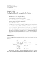
Báo cáo hóa học: " Research Article Static Object Detection Based on a Dual Background Model and a Finite-State Machine Rub´ n Heras Evangelio and Thomas Sikora e" doc
Bạn đang xem bản rút gọn của tài liệu. Xem và tải ngay bản đầy đủ của tài liệu tại đây (7.27 MB, 11 trang )
Hindawi Publishing Corporation
EURASIP Journal on Image and Video Processing
Volume 2011, Article ID 858502, 11 pages
doi:10.1155/2011/858502
Research Ar ticle
Static Object Detection B ased on a Dual
Background Model and a Finite-State Machine
Rub
´
en Heras Evangelio and Thomas Sikora
Communication Systems Group, Technical University of Berlin, D-10587 Berlin, Germany
Correspondence should be addressed to Rub
´
en Heras Evangelio,
Received 30 April 2010; Revised 11 October 2010; Accepted 13 December 2010
Academic Editor: Luigi Di Stefano
Copyright © 2011 R. Heras Evangelio and T. Sikora. This is an open access article distributed under the Creative Commons
Attribution License, which permits unrestricted use, distribution, and reproduction in any medium, provided the original work is
properly cited.
Detecting static objects in video sequences has a high relevance in many surveillance applications, such as the detection of
abandoned objects in public areas. In this paper, we present a system for the detection of static objects in crowded scenes. Based on
the detection of two background models learning at different rates, pixels are classified with the help of a finite-state machine. The
background is modelled by two mixtures of Gaussians with identical parameters except for the learning rate. The state machine
provides the meaning for the interpretation of the results obtained from background subtraction; it can be implemented as a look-
up table with negligible computational cost and it can be easily extended. Due to the definition of the states in the state machine,
the system can be used either full automatically or interactively, making it extremely suitable for real-life surveillance applications.
The system was successfully validated with several public datasets.
1. Introduction
Detecting static objects in video sequences has several
applications in surveillance systems such as the detection
of illegally parked vehicles in traffic monitoring or the
detection of abandoned objects in public safety systems and
has attracted the attention of a vast research in the field of
video surveillance. Most of the proposed techniques aiming
to detect static objects base on the detection of motion,
achieved by means of background subtraction, followed
by some kind of tracking [1]. Background subtraction
is a commonly used technique for the segmentation of
foreground regions in video sequences taken from a static
camera, which basically consists on detecting the moving
objects from the difference between the current frame and a
background model. In order to achieve good segmentation
results, the background model must be regularly kept
updated so as to adapt to the varying lighting conditions and
to stationary changes in the scene. Therefore, background
subtraction techniques often do not suffice for the detection
of stationary objects and are thus supplemented by an
additional approach.
Most of the approaches suggested in the recent literature
for the detection of static objects rely on tracking informa-
tion [1–4]. As observed by Porikli et al., [5]. these methods
can find difficulties in real-life scenes involving crowds due
the large amounts of occlusions and to the shadows casted
by moving objects, which turn the object initialization and
tracking into a hard problem to solve. Many of the appli-
cations where the detection of abandoned objects can be of
interest like safety in public environments (airports, railway
stations) impose the requirement of coping with crowds.
In order to address the limitations exhibited by tracking-
based approaches, Porikli et al. [5]. proposed a pixelwise
system which uses dual foregrounds. Therefore, they used
two background models with different learning rates, a
short-term and a long-term background model. In this way,
they were able to control how fast static objects get absorbed
by the background models and detect them as those groups
of pixels classified as background by the short-term but not
by the long-term background model.
A drawback of this system is that temporarily static
objects may also become absorbed by the long-term back-
ground model after a given time depending on its learning
2 EURASIP Journal on Image and Video Processing
rate. This would lead the system to not detect those static
objects anymore and furthermore to detect the uncovered
background regions as abandoned objects when they are
removed from the scene. To overcome this problem, the
long-term background model could be updated selectively.
The disadvantage of this approach is that incorrect update
decisions might later result in incorrect detection and that
the uncovered background could be detected as foreground
after removing static objects even if those do not get
absorbed by the long-term model if the lighting conditions
have changed notably.
The combination of the foreground masks obtained from
the subtraction of two background models was already used
by [6] in order to quickly adapt to changes in the scene
while preventing foreground objects from being absorbed
too fast by the background model. They used the intersection
of the foreground masks to selectively update the short-term
background model, obtaining a very precise segmentation
of moving objects, but they did not consider the problem
of detecting new static objects. Recently, Singh et al. [4]
proposed a system for the detection of static objects that
also bases on two background models however; it relies
on selectively updating the long-term background model,
entailing the above-mentioned problem of possibly taking
incorrect updating decisions, and on tracking information.
To solve the problem that poses static objects concerning
the updating of the long-term background model in dual
background systems, we propose a system that, based on the
results obtained from a dual background model, classifies
the pixels according to a finite-state machine. Therefore, we
can define the meaning of obtaining a given result from
background subtraction when being in a given state. Thus,
thesystemisabletodifferentiate between background and
static objects that have been absorbed by both background
models depending on the pixels history. Furthermore, by
adequately designing the states and transitions of the finite-
state machine, the system that we define can be used either
in a full automatic or in an interactive manner, making
it extremely suitable for real-life surveillance applications.
After classification, pixels are grouped according to their
class and connectivity. The content of this paper has been
partially submitted to the IEEE Workshop on Applications of
Computer Vision (WACV) 2011 [7] . In the present paper, we
provide a detailed insight into the proposed system and some
robustness and efficiency implementation issues to further
enhance it.
The rest of this paper is organized as follows In Section 2
we briefly describe the task of background subtraction, which
sets the basis of our system. Section 3 is devoted to the finite-
state machine, including some implementation remarks.
Section 4 summarizes some experimental results and the
limitations and merits of the proposed system. Section 5
concludes the paper.
2. Background Modelling
Background subtraction is a commonly used approach to
detect moving objects in video sequences taken from a static
camera. In essence, for every pixel
{x, y} at a given time t,
the probability of observing the value X
t
= I(x, y, t), given
the pixel history X
T
={X
t
, , X
t−T
},isestimated
P
(
X
t
| X
T
)
,(1)
andthepixelisclassifiedasbackgroundifthisprobability
is bigger than a given threshold or as foreground if not.
The estimated model in (1) is known as background
model and the pixel classification process as background
subtraction. The classification process depends on the pixel
history as explicitly denoted in (1). In order to obtain a
sensitive detection, the background model must be updated
regularly to adapt to varying lighting conditions. Therefore,
the background model is a statistical model containing
everything in a scene that remains static and depends on the
training set X
T
used to build it. A study of some well-known
background models can be found in [8–10] and references
therein.
As observed in [11], there are many surveillance scenarios
where the initial background contains objects that are
later removed from the scene (parked cars, static persons
thatmoveaway,etc.).Whentheseobjectsmoveaway,
they originate a foreground blob that should be correctly
classified as a removed object. Although this is an important
classification step for an autonomous system, we do not
consider this problem in this paper. We assume that, after
an initialization time, the background model only contains
static objects which do belong to the empty scene. Some
approaches on background initialization can be found in [12,
13] and references therein. In [12], the authors use multiple
hypotheses for the background at each pixel by locating
periods of stable intensity during the training sequence. The
likelihood of each hypothesis is evaluated by using optical
flow information from the neighboring pixels. The most
likely hypothesis is chosen as background model. In [13]
the background is estimated in a patch by patch manner by
selecting the most appropriate candidate patches according
to the combined frequency responses of extended versions of
candidate patches and their neighbourhood, thus exploiting
spatial correlations within small regions.
The result of a background subtraction is a foreground
mask F, which is a binary image where the pixels classified
as foreground are differentiated from those classified as
background. In the following, we use the value 1 for those
pixels classified as foreground (foreground pixels), and 0
for those classified as background (background pixels).
Foreground pixels can be grouped into blobs by means
of connectivity properties [14, 15]. Blobs are foreground
regions which can belong to one or more objects or even
to some parts of different objects in case of occlusions.
For brevity in the exposition, we will refer to the detected
foreground regions as objects. Accordingly, we will use the
term static objects instead of the more precise form static
foreground regions.
2.1. Dual Background Models. A statistical background
model as defined in (1) provides a description of the
static scene. Since the model is updated regularly, objects
EURASIP Journal on Image and Video Processing 3
Table 1: Hypotheses based on the long-term and short-term
foregroundsasin[5].
F
L
(X
t
) F
S
(X
t
)Hypothesis
11 Movingobject
1 0 Candidate abandoned object
0 1 Uncovered background
00 Scenebackground
being introduced in the scene and remaining static will
be incorporated into the model at some time. Therefore,
regulating the training set X
T
orthelearningrateusedto
build the background model, it is possible to adjust how
fast new static objects get incorporated into the background
model.
Porikli et al. [5] used this fact to detect new static
objects based on the foreground masks obtained from two
background models learning at different rates, a short-term
foreground mask F
S
, and a long-term foreground mask
F
L
.F
L
shows the pixel values corresponding to moving
objects and temporarily static objects, as well as shadows
and illumination changes that the long-term background
model fails to incorporate. F
S
contains the moving objects
and noise. Depending on the foreground masks values, they
postulate the hypotheses shown in Table 1,whereF
L
(X
t
)
and F
S
(X
t
) denote the value of the long-term and short-
term foreground mask at pixel X
t
, respectively. We use this
notation in the rest of this paper.
After a given time according to the learning rate of
the long-term background, the pixel values corresponding
to static objects will be learned by this model too, so
that, following the hypotheses in Table 1, those pixels will
be hypothesized from this time on as scene background.
Moreover, if any of those objects get removed from the scene
after their pixel values have been learned by the long-term
background, the potential background may be detected as a
static object.
In order to handle those situations, we propose in this
paper a system that, based on the foreground masks obtained
by the subtraction of two background models learning at
two different rates, hypothesizes on the pixel classification
according to the last pixel classification. This system is
formulated as a finite-state machine where the hypotheses
depend on the state of a pixel at a given time, and the condi-
tions are the results obtained from background subtraction.
As background model,we use two improved Gaussian
mixture models as described in [16] initialized with identical
parameters except for the learning rate, a short-term back-
ground model B
S
, and a long-term background model B
L
.
Actually, we could use any parametrical multimodal back-
ground model (see [17], e.g.) that do not alter the parameters
of the distribution that represents the background when a
foreground object hides it.
The background model presented in [16] is very similar
to the well-known mixture of Gaussians model proposed
in [18]. In a nutshell, each pixel is modelled as a mixture
of a maximum number N of Gaussians. Each Gaussian
distribution i is characterized by an estimated mixing weight
ω
i
, a mean value, and a variance. The Gaussian distributions
are sorted attending to their mixing weight. For every
new frame, each pixel is compared with the distributions
describing it. If there exists a distribution that explains this
pixel value, the parameters of the distribution are updated
according to a learning rate α as expressed in [16]. If not,
a new one is generated with mean value equal to the pixel
value and weight and variance set to some fixed initialization
value. The first B distributions are chosen as the background
model, where
B
= arg min
b
⎛
⎝
b≤N
i=1
ω
i
> B
⎞
⎠
,(2)
with B being a measure of the minimum portion of the data
that should be considered as background. After each update,
the components that are not supported by the data, that is,
these with negative weights, are suppressed and the weights
of the remaining components are normalized in a way that
theyadduptoone.
3. Stat ic Objects Detection
As we show in Section 2, a dual background model is not
enough to detect static objects for an arbitrarily long period
of time. Consider a pixel X
t
being part of the background
model (the pixel is thus classified as background) and the
same pixel X
t+1
atthenexttimestept + 1 being occluded
by a foreground object. The value of both foreground masks
F
S
(X
t+1
)andF
L
(X
t+1
)att + 1 will be 1. If the foreground
object stays static, it will be learned by the short-term
background model at first (let us assume at t + α, F
S
(X
t+α
) =
0andF
L
(X
t+α
) = 1) and afterwards by the long-term
background (let us assume at t + β, F
S
(X
t+β
) = 0and
F
L
(X
t+β
) = 0). This process can be graphically described as
shown in Figure 1.
If we further observe the behavior of the background
model of this pixel in time, we can transfer the meaning of
obtaining a given result from background subtraction after
a given history into pixel classification hypothesis (states)
and establish which transitions are allowed from each state
and what are the inputs needed to cause these transitions.
In this way, we can define the state transitions of a finite-
state machine, which can be used to hypothesize on the pixel
classification.
As we will see in the following subsections, there are
some states that require additional information in order to
determine what is the next state for a given input. In these
cases it is necessary to know if any of the background models
gives a description of the actual scene background and, in
affirmative case, which of them. Therefore, we keep a copy
of the last background value observed at every pixel position.
This value will be used, for example, to distinguish when a
static object is being removed or when it is being occluded by
another object. In this sense, the finite-state machine (FSM)
presented in the following can be considered as an extended
finite-state machine (EFSM), which is an FSM extended with
input and output parameters, context variables, operations
and predicates defined over context variables and input
4 EURASIP Journal on Image and Video Processing
(F
L
, F
S
) = (0, 0) (F
L
, F
S
) = (1, 1) (F
L
, F
S
) = (1, 0) (F
L
, F
S
) = (0, 0)
(F
L
, F
S
) = (1, 1)
T
= t +1
(F
L
, F
S
) = (1, 0)
T
= t + α
(F
L
, F
S
) = (0, 0)
T
= t + β
T
= tt+1<T<t+ αt+ α<T<t+ βT>t+ β
BG MP PAP AP
Figure 1: Graphical description of the states a pixel goes through when being incorporated into the background model. BG indicates a pixel
that belongs to the background model, MP a pixel that belongs to a moving object, PAP a partially absorbed pixel, and AP an absorbed pixel.
00
11
00
10 00
01
10
00
01
01
11
11, 01
10
01
11
10
00
11
00
10
01
00
00
11,10
10
01
11
11
00
11
10
00
01
11
01
01
10
10
01 and ev10
00 and ev4
00 and ev0
10 and ev9
10 and ev7
01 and
ev3
UAP
10
BG
0
MP
1
UBG
3
PAP
2
AP
4
NI
5
OULKBG
8
AI
6
ULKBG
7
PAPAP
9
Otherwise
Go to 8
(OULKBG)
Go to 6
(AI)
Go to 6
(AI)
Go to 3
Figure 2: Next state function of the proposed finite-state machine.
parameters [19]. An EFSM can be viewed as a compressed
notation of an FSM, since it is possible to unfold it into
a pure FSM, assuming that all the domains are finite [19],
which is the case in the state machine presented here. In fact,
we make use of context variables in a very limited number
of transitions. Therefore, for clarity in the presentation, we
prefer to introduce the state-machine as an FSM at first and
then remark where the EFSM features are exploited.
In the following subsection we present the FSM in its
general form. Section 3.2 outlines how the results of the FSM
can be used by higher layers in a computer vision system.
Section 3.3 presents how the FSM can be further enhanced
intermsofrobustnessandefficiency.
3.1. A Finite-State Machine for Hypothesizing on the Pixel
Classification. A finite-state machine describes the dynamic
behavior of a discrete system as a set of input symbols, a
set of possible states, transitions between those states, which
are originated by the inputs, a set of output symbols, and
sometimes actions that must be performed when entering,
leaving or staying in a given state. A given state is determined
by past states and inputs of the system. Thus, an FSM
can be considered to record information about the past of
the system it describes. Therefore, by defining a state machine
whose states are the hypothesis on the pixels and whose
inputs are the values obtained from background subtraction,
we can record information about the pixel history and
thus hypothesize on the classification of a pixel given a
background subtraction result depending on the state where
it was before.
An FSM can be defined as a 5-tuple (I, Q, Z,δ, ω)[20],
where
(i) I is the input alphabet (a finite set of input symbols),
(ii) Q is a finite set of states,
(iii) Z is the output alphabet (a finite set of output
symbols),
(iv) δ is the next-state function, a mapping of I
× Q into
Q,and
(v) ω is the output function, a mapping of I
×Q onto Z.
We d efi ne :
(a) I to be the possible combinations of the results
obtained from background subtraction. By defining
the pair (F
L
, F
S
), the input alphabet reduces to I ≡
{
(0, 0),(0,1), (1,0), (1,1)};
(b) Q to be the set of states a pixel can go through as
described below;
EURASIP Journal on Image and Video Processing 5
(c) Z to be either a set of numbers indicating the hypoth-
esis on the pixel classification Z
≡{0, 1, |Q|},with
|Q| being the cardinality of Q, or a boolean output
Z
≡{0,1} with the value 0 for pixels not belonging
to a static object and 1 for pixels belonging to a
static object. Choosing the output alphabet depends
on whether the hypotheses of the machine are to be
further interpreted or not;
(d) δ to be a next-state function as depicted in Figure 2.
(e) ω to be the output function. This can be either
a multivalued function with output values z ∈
{
0, 1, |Q|} corresponding to the state of a pixel at
a given time, or a boolean function with output 0 for
pixels not belonging to a static object and 1 for pixels
belonging to a static object.
Additionally, we keep a copy of the last background value
observed at every pixel position.
In the following, we list the states of the state machine,
their hypothetical meaning, the condition that must be met
to enter them, or to stay in them and a brief description of
their meaning:
(0) (BG), background,(F
L
, F
S
) = (0, 0). The pixel belongs
to the scene background,
(1) (MP), moving pixel,(F
L
, F
S
) = (1,1). The pixel
belongs to a moving object. This state can be reached as well
by pixels belonging to the background scene being affected by
spurious noise not characterized by the background model,
(2) (PAP), partially absorbed pixel,(F
L
, F
S
) = (1, 0). The
pixel belongs to an object that has already been absorbed by
B
S
but not by B
L
. In the following, we refer to these objects as
short-term static objects,
(3) (UBG), uncovered background,(F
L
, F
S
) = (0,1). The
pixel belongs to a background region that was occluded by a
short-term static object,
(4) (AP), absorbed pixel,(F
L
, F
S
) = (0,0). The pixel
belongs to an object that has already been absorbed by B
S
and B
L
. In the following, we refer to these objects as long-
term static objects,
(5) (NI), new indetermination,(F
L
, F
S
) = (1, 1). The pixel
cannot be classified as background neither by B
S
nor by B
L
.
It is not possible to ascertain if the pixel corresponds to a
moving object occluding a long-term static object or if a
long-term static object was removed. We do not take any
decision at this moment. If the pixel belongs to a moving
object occluding a long-term static object, the state machine
will jump back to AP when the moving object moves out.
If not, the “new” color will be learned by B
S
and the state
machine will jump to AI, where a decision will be taken,
(6) (AI), absorbed indetermination,(F
L
, F
S
) = (1, 0). The
pixel is classified as background by B
S
but not by B
L
.Given
the history of the pixel it is not possible to ascertain if any of
the background models gives a description of the actual scene
background. To solve this uncertainty, the current pixel value
is compared to the last known background value at this pixel
position. We discuss below how to obtain and update the last
known background value,
(7) (ULKBG), uncovered last known background,
(F
L
, F
S
) = (1, 0). The pixel is classified as background by
B
S
but not by B
L
and identified as belonging to the scene
background,
(8) (OULKBG), occluded uncovered last known back-
ground,(F
L
, F
S
) = (0, 1). The pixel is classified as background
by B
L
but not by B
S
,andB
S
is known to contain a
representation of the scene background. This state can be
reached when a long-term static object has been removed, the
actual scene background has been learned again by B
S
and an
object whose appearance is very similar to the removed long-
term static object occludes the background,
(9) (PAPAP), partially absorbed pixel over absorbed pixel,
(F
L
, F
S
) = (1, 0). The pixel is classified as background by
B
S
but not by B
L
and could not be identified as belonging
to the scene background. Therefore, it is classified as a pixel
belonging to a short-term static object occluding a long-term
static object,
(10) (UAP), uncovered absorbed pixel,(F
L
, F
S
) = (0, 1).
The pixel is classified as background by B
L
but not by B
S
,and
B
L
could not be interpreted to contain a representation of
the actual scene background. This state can be reached when
a short-term static object was occluding a long-term static
object and the short-term static object gets removed.
Observe that we need additional information in order
to determine the transitions from state 6. This is due to
the fact that it is not possible to ascertain if any of the
background models gives a good description of the actual
scene background. To illustrate this, let us consider two cases:
a long-term static object getting removed and a long-term
static object getting occluded by a short-term static object.
In both cases, when the long-term static object is visible
B
S
and B
L
classify it as background (state 4, (F
L
, F
S
) =
(0, 0)). Afterwards, when the long-term static object gets
removed or occluded, a “new” color is observed. The “new”
color persists at this pixel position, and it gets first learned
by B
S
(state 6, (F
L
, F
S
) = (1,0)), causing an uncertainty,
since it is impossible to distinguish if the “new” color
corresponds to the scene background or to a short-term
static object occluding the long-term static object. To solve
this uncertainty, we compare the current pixel value with
the last known background value at this pixel position. In
this state the FSM is actually behaving as an EFSM, and the
copy of the last background value observed at this position
is a context variable. Since this is the unique state where the
FSM explicitly makes use of extended features, we decided to
remark that aside in order to keep the description of the state
machine as simple as possible.
The last known background value is initialized for each
pixel after the initialization phase of the background models.
How to initialize a background model is out of the scope of
this paper. In Section 2, we give references on papers dealing
with this topic. This value is subsequently updated for every
pixel position when a transition from BG (state 1) is triggered
as follows:
if
(
F
L
, F
S
)
=
(
0, 1
)
, b
LK
(
X
)
= B
L
(
X
)
,
otherwise, b
LK
(
X
)
= B
S
(
X
)
,
(3)
where b
LK
denotes the last known background value.
6 EURASIP Journal on Image and Video Processing
MPIII
15
BG
0
MP
1
PAP
2
AP
4
PAPII
14
MPII
13
OULKBGII
11
UBGII
12
Go to AI (6)
Go to AI (6)
Go to
AI (6)
Go to
AI (6)
Go to
AI (6)
Go to UAP (10)
Go to
ULKBG (7)
UBG
3
00
10
01
00
11
00
00
10
01
10
01
11
10
00
11
10
01
1101
00
11
00
10
01
00
01, 11
10
10
00
00
11
11
01
01
10
01
10
11
Figure 3: Five additional states and six additional conditions on transitions to enhance the robustness and the efficiency of the FSM shown
in Figure 2.
The output function of the FSM can have two forms:
(i) a boolean function with output 0 for nonstatic pixels
and 1 for static pixels. In this case, it has to be
decided which subset O of Z designates a static
pixel. There are many possibilities, depending on the
desired responsiveness of the system. The lower and
higher responsiveness are achieved by O
≡{4} and
O
≡{2, 4,5,6,8,9, 10}, respectively;
(ii) A multivalued function with output values q
∈
{
0, 1, |Q|} corresponding to the state where the
pixel is at a given time.
At the moment, we use a subset of Z to classify groups
of pixels as static objects, but we used the second form in
order to provide some examples of the classification states
obtained. Furthermore, the results obtained by using a multi-
valued function can be used to feed up a second-layer group-
ing pixels by means of their hypotheses and build objects.
3.2. Grouping Pixels into Objects. The state of each pixel at a
given time t provides a rich information that can be further
processed to refine the hypothesis. Pixels can be spatially
combined depending on their states and their connectivity.
At the moment, we take those pixels in the states 4 and 5
and those that have been in the states 2 or 9 for more than
a given time threshold T and group them attending to their
connectivity. Those groups of pixels bigger than a fixed size
are then classified as static objects.
3.3. Robustness and Efficiency Issues. The FSM introduced in
Section 3.1 provides a reliable tool to hypothesize on the
meaning of the results obtained from a dual background
subtraction. However, there are some state-input sequences
where an additional computation must be done in order to
decide on the next state, namely when the state machine
arrives at the state AI (6). A state-input sequence entering the
state AI is AP-(1,1)
→ NI-(1,0) → AI, which corresponds to
a pixel of a long-term static object being removed or getting
occluded by a short-term static object. In this situation
it is necessary to disambiguate the results obtained from
background subtraction.
Therearethreemorestate-inputsequencesenteringthe
state AI, where this extra computation can be eventually
avoided. These are MP-(0,1)
→ OULKBG-(1,1) → AI,
UBG-(1,1)
→ AI, and PAP-(1,1) → AI. In fact, these
sequences enter the state AI because they can derive in a state
input where a disambiguation is necessary, given the pixel
history. Therefore, if we define known sequences starting at
the first state-input pair of the three sequences mentioned
above, we can avoid reaching AI for these known sequences.
In order to do that, we added five more states to the FSM:
(11) (OULKBGII), occluded uncovered last known back-
ground ii,(F
L
, F
S
) = (0, 1),
(12) (UBGII), uncovered background ii,(F
L
, F
S
) = (1, 0),
(13) (MPII), moving pixel ii,(F
L
, F
S
) = (1, 1),
(14) (PAPII), partially absorbed pixel ii,(F
L
, F
S
) = (1, 0),
(15) (MPIII), moving pixel iii,(F
L
, F
S
) = (1, 1).
EURASIP Journal on Image and Video Processing 7
These states are specializations of the states they inherit
their name from and have the sense of avoiding to enter
the state AI in these situations where the meaning of the
state-input sequence is non ambiguous. Therefore, we call
them known sequences. Their meaning can be inferred out
of the transitions shown in Figure 3 and of the state they
specialize. In this fashion some additional specialized states
can be defined.
Figure 3 also shows six additional conditions on six
transitions marked as an orange point on the respective
transition arrows. The reason why we introduce these
conditions here is that the tuple (F
L
(X
t
), F
S
(X
t
)) at time
step t does not really make sense if being in the state where
the transitions are conditioned. Thus, we hypothesized that
it was obtained because of noise and “stay” at the current
state. If the tuple (F
L
(X
t+1
), F
S
(X
t+1
)) in the next time step
t +1isequalto(F
L
(X
t
), F
S
(X
t
)), then the conditioned
transition is done. In practice, these additional conditions
are implemented as replica states with identical transitions
as the state being replicated except for the transition being
conditioned, which is only done in the corresponding replica
state (the replicated state transitions to the replica state). We
do not represent these replica states in the next-state function
graph for clarity.
Introducing additional states enhances the robustness
of the state machine, since there are less input sequences
deriving in state AI. Thus, there are less pixels that have
to be checked with an eventually old version of the scene
background (the last known background value is updated
when a transition leaving the state BG is). Furthermore,
because of avoiding this additional computation, we gain
in efficiency. Replica states also contribute to enhance the
performance of the system, since they filter out noisy inputs.
4. Exp erimental Results
In this section, we present results obtained with the proposed
system and with a dual background-based system that does
not use an FSM (pixels are classified by using the hypotheses
shown in Table 1 and an evidence value in a similar way
as proposed in [5]), which we use as reference system. To
abbreviate, we will refer to those systems as DBG+FSM and
DBG+T, respectively.
To test the systems, we used three public datasets: i-
LIDS, PETS2006 and CAVIAR. The sequences AB-Easy, AB-
Medium and AB-Hard from the i-LIDS dataset show a scene
in an underground station. In PETS2006, there are several
scenes from different camera views of a closed space; we
took the scene S1-T1-C-3. CAVIAR covers many different
events for scene interpretation of interest in a video surveil-
lance application (people fighting, people/groups meeting,
walking together and splitting up, or people leaving bags
behind ), taken from a high camera view; from this dataset
we took the scene LeftBag. The scenes from i-LIDS became
our major attention, since they show one of the challenges
that we tackle on this paper, namely a static object being for a
long time in the scene and then being removed. However, the
scenes AB-Medium and AB-Hard present the handicap that
the static scene cannot be learned before the static objects
come into the scene, which is a requirement for both systems
(DBG+T and DBG+FSM); therefore, we added 10 frames
showing the empty scene at the beginning of each scene,
respectively, in order to train the background models. In
PETS2006, static objects are not removed, and thus, even if
the static objects have to be detected, they do not pose the
problem of detecting when a static object has been removed.
In the CAVIAR scene LeftBag, static objects are removed
that early, that every background model can be tuned not
to absorb them without risking the responsiveness of the
background model. Thus, we do not consider these two last
sets of scenes very challenging for the task of static objects
detection. We nevertheless chose these three datasets, since
they are the most commonly used in the computer vision
community for the presentation of systems for the detection
of static objects.
As background model, we used two Gaussian mixture
models with shadow detection. A comprehensive description
of the model can be found in [16]. We set up both
background models with identical parameters except for the
learning rate. The learning rate of the short-term model B
S
is 10 times the learning rate of the long-term model B
L
.
We consciously chose a relatively large value for α
L
to force
B
L
to learn the static objects in the scene and thus being
able to prove the correct operation of the proposed system
both when static objects are learned by B
L
and when they
get removed from the scene. It is important thus to remark
that the goal of the experiments presented here is to evidence
what problems double background-based systems face on the
detection of long-term static objects and how the proposed
approach solves them. Therefore, we had to cope with objects
getting very fast classified as static. In practice, α
L
can be
drastically reduced. The rest of the parameters were chosen
as follows:
(i) σ
init
= 11,
(ii) σ
thres
= 3,
(iii) B
= 0.05, which means that only the first component
of the background model is taken as background,
where σ
init
is the initialization value for the variance of a
new distribution, and σ
thres
is the threshold value for a pixel
to be considered to match a given distribution. These are
the most commonly used values in papers reporting the
use of Gaussian mixture models for the task of background
subtraction.
The masks obtained from background subtraction were
taken without any kind of postprocessing as input for the
FSM. We let the background models learn for a period of
10 frames and, assuming that at this time the short-term
background already has a model of the scene background,
start the state machine.
The FSM was implemented as a lookup table and is
thus very low demanding in terms of computation time.
Only at state AI extra computations are needed. At this
step, we use a voting system to decide the next state for a
given input, by comparing the pixel against the last value
seen for background at this pixel and impose the condition
8 EURASIP Journal on Image and Video Processing
of obtaining a candidate state at least five times. For this
comparison, we used a context variable. Wedo not define this
comparison as an input of the state machine, since it is only
needed for pixels being in this state. Therefore, we save the
computational cost of computing a third foreground mask
based on this background model.
Pixel classification was made taking the pixels whose
FSMs were in the states AP and NI, or in the states PAP
and PAPAP for a time longer than 800 frames and building
connected components. To build connected components
we used the CvBlobsLib, available at />projects/cvblobslib/, which implements the algorithm in
[21]. Groups of pixels bigger than 200 pixels were classified as
static objects. Time and size thresholds were changed for the
LeftBag sequence, according to the geometry and challenge
of the scene. While in the PETS and iLIDS sequences a
rucksack can be bounded with a 45
× 45 pixels box, a
rucksack of the approximately same size takes because of
the frame size a box of only 20
× 20 pixels in the CAVIAR
sequences. Moreover, the LeftBag sequence of CAVIAR poses
the challenge of detecting static objects being in the scene for
385 frames, what would make no sense in a subway station
(iLIDS sequences), since almost each waiting person would
trigger an alarm.
Ta b l e 2 presents some results obtained with the proposed
system and with DBG-T. True detections indicate that an
abandoned object was detected. False detections indicate
that an abandoned object was detected where, in fact, there
was not an abandoned object (but, for example, a person).
Missed detections indicate that an abandoned object was not
detected. Lost detections indicate correctly detected static
objects that were not detected anymore after a given time
because of being absorbed by the long-term background
model. We detected successfully all static objects. While we
report some false detections in the AB-Medium and AB-
Hard sequences, these detections do correspond in every case
to static objects (persons staying static for a long time); we
rated them as false detections, since they do not correspond
to abandoned objects.
We detected successfully all static objects. The false
detections in the AB-Medium and AB-Hard sequences
correspond in every case to persons staying static for a long
time. These detections can be ignored by incorporating an
object classifier in order to discard people staying static for
a long time (this classification step will be incorporated in
future work). Furthermore, notice that we set a learning
rate for B
L
larger than needed in order to prove the correct
operation of the FSM, which is also partially the cause of
static objects being detected that fast.
Figures 4, 5 and 6 show some examples obtained for the
i-LIDS sequences. Pixels are colored according to the colors
of the states shown in Figure 2. Pixels belonging to moving
objects are painted in green, pixels belonging to short-term
static objects in yellow, and so on. The second frame of each
sequence shows how time can be used to mark short-term
static objects as static. The third frames show how long-term
static objects (in red) are still being detected (these objects get
lost by a DBG-T system if not additionally using some kind
of selective updating scheme for the long-term background
model). In the AB-Medium and AB-Hard sequences it is
also shown the robustness of the proposed system against
occlusions in crowded scenes. The fourth frames show the
starting of the disambiguation process when long-term static
objects get removed. The fifth frames show how the static
object detection stops when the scene background is again
identified as such.
The processing time needed can slightly vary depending
on the scene complexity and on the configuration of the
underlying background model. A very complex background
scene requires more components and thus more compu-
tation time. Moreover, when long-term static objects get
absorbed by the long-term background and afterwards get
removed, an indetermination state has to be solved. Beyond
that, the more static objects there are, the more the blobs
generation costs. To give an idea, what the computational
times are, we report in Table 3 the average frame processing
time in miliseconds and in frames per second for the i-
LIDS sequences AB-Easy, AB-Medium, AB-Hard and an
average over the PETS2006 dataset, running in an Intel
Core2 Extreme CPU X9650 at 3.00 GHz without threading.
Since each pixel is considered individually, the processing
described here can be easily implemented in a parallel
architecture, gaining considerably in speed. In the i-LIDS
sequences we only analyzed the platform (that means,
339.028 pixels out of 414.720). The frames of the PETS2006
dataset were taken as they are (that means a total amount of
414.720 pixels per frame). We show processing times for the
update of a double background system (DBG), for the DBG-
T system, and for the proposed system (DBG-FSM).
It is apparent that the proposed method outperforms
the DBG-T system in terms of detection accuracy while
having similar processing demands. Table 3 shows that the
computational time needed for the update of the state
machine is very low compared to the time needed for the
update of the background model. The processing time of
the proposed system was always lower when using a state
machine with the enhancements proposed in Section 3.3,but
the most important advantage of using specialized states is
that the state machine of many pixels does not go to states
in which an indetermination has to be solved, as shown in
Figure 7. The times reported show that the system can run in
real time in surveillance scenarios.
4.1. System Limitations and Merits. The system presented
here aims to detect static objects in a video sequence that
do not belong to the scene background. As such, the actual
scenebackgroundmustbeknownwhenthestatemachine
starts working, which is a realistic requirement for real-
life applications. Furthermore, we do not use any kind of
object models in order to distinguish, for instance, persons
waiting in a bank from other kind of static objects. Neither
tracking information was used to trigger “drop-off ”alarms
in a similar fashion as Guler and Farrow do in [22], which
could be coupled with our system in form of a parallel layer
in order to bring a kind of semantic for scene interpretation.
Static objects would still be detected with no need of tracking
information, while a higher layer could fuse incoming
EURASIP Journal on Image and Video Processing 9
Table 2: Detection results of the DBG-T and the proposed system (DBG-FSM).
Scene
True detections False detections Missed detections Lost detections
DBG-T DBG-FSM DBG-T DBG-FSM DBG-T DBG-FSM DBG-T DBG-FSM
AB-Easy11000010
AB-Medium11550010
AB-Hard11660010
cam3 11000010
LeftBag11000000
Figure 4: Pixel classification in five frames of the scene AB-Easy. Frame number from left to right: 1967, 3041, 4321, 4922, and 5098.
Figure 5: Pixel classification in five frames of the scene AB-Medium. Frame number from left to right: 951, 3007, 3900, 4546, and 4715.
Figure 6: Pixel classification in five frames of the scene AB-Hard. Frame number from left to right: 251, 2335, 3478, 4793, and 4920.
Table 3: Processing time needed for the update of a double
background model (DBG), for the DBG-T system, and for the
proposed system (DBG-FSM) in miliseconds (ms) and frames per
second (fps).
Scene
DBG DBG-T DBG-FSM
msfpsmsfpsmsfps
AB-Easy 59.30 16.86 62.18 16.08 63.27 15.80
AB-Medium 67.62 14.79 70.57 14.17 72.28 13.84
AB-Hard 68.30 14.64 71.23 14.04 71.87 13.91
PETS2006 60.77 16.46 63.41 15.77 64.58 15.48
information from several cues in order to make a semantic
scene interpretation. As pointed out, the system presented
here is restricted to the detection of static objects which do
not belong to the scene background.
AsshowninFigure2, the condition for the FSM to stay
at the state AP at a given pixel X
t
is that (F
L
(X
t
), F
S
(X
t
)) =
(0, 0), which is the same condition as the one to stay at
BG. That means that if a piece of the scene background
was wrongly classified as static object, an operator could
interactively correct this mistake with no need for the system
to correct any of the background models, since those are
updated regularly in a blind fashion. This could happen, for
example, if a static object has occluded the background that
long, that the last known background is not similar anymore
to the scene background when the object is removed because
of a lighting change. This is a huge advantage of our
system in comparison to other systems based on selectively
updating the background model, not only because we avoid
wrong update decisions but also because the system provides
the possibility of incorporating interactive corrections with
no need of modifying the background model. Thus, the
background model remains as a pure statistical information.
The same applies for static objects that an operator
can be considered noninteresting, which is a common
issue in open spaces, where waste containers and other
static objects are moved in the scene but do not represent
a dangerous situation. Static object detection approaches
10 EURASIP Journal on Image and Video Processing
(a) (b)
Figure 7: Detail of pixel classification when using specialized states
(a) and not (b).
Figure 8: Crop of frame nr. 4158 (i-LIDS AB-Hard).
based on selective updating of the background model do not
offer a principled way of incorporating such items into the
background model. Since our background model is updated
in a blind fashion, these objects do get incorporated into
the background model. Only the state of the FSM has to be
changed. This kind of interaction can be defined as well with
other layers in a complex computer vision system.
A further extension of the system can be to use infor-
mation of neighboring pixels to discard some detected static
objects. Based on the observation that the inner pixels of
slightly moving objects are learned by B
L
and B
S
faster
than the outer pixels (especially by uniform colored objects),
it can be differentiated between static objects and slightly
moving objects by grouping neighboring pixels. This can be
implementedasasecondlayerwhichresultscanevenbe
feedback as an additional input in order to help solving some
indeterminations at state AI. Figure 8 shows a detected static
object that can be discarded following this criterion.
5. Conclusions
In this paper we presented a robust system for the detection
of static objects in crowded scenes without the need of any
tracking information. By transferring the meaning of obtain-
ing a given result from background subtraction after a given
history into transitions in a finite-state machine, we obtain a
rich information that we use for the pixel classification. The
state machine can be implemented as a lookup table with
negligible computational cost, it can be easily extended to
accept more inputs and can also be coupled with parallel
layers in order to extract semantic information in video
sequences. In fact, the proposed method outperforms the
reference system in terms of detection accuracy while having
similar processing demands. Due to the condition imposed
for a pixel to remain classified as static in a long-term basis,
the system can be interactively corrected by an operator
without need for the system to modify anything in the back-
ground models, what alleviates the system from persistent
false classification originated by incorrect update decisions
in contrast to selective updating-based systems. The system
was successfully validated with several public datasets.
References
[1] A. Bayona, J. C. SanMiguel, and J. M. Mart
´
ınez, “Compar-
ative evaluation of stationary foreground object detection
algorithms based on background subtraction techniques,”
in Proceedings of the 6th IEEE International Conference on
Advanced Video and Signal Based Surveillance (AVSS ’09),pp.
25–30, September 2009.
[2]S.Guler,J.A.Silverstein,andI.H.Pushee,“Stationary
objects in multiple object tracking,” in Proceedings of the IEEE
Conference on Advanced Video and Signal Based Surveillance
(AVSS ’07), pp. 248–253, September 2007.
[3] P. L. Venetianer, Z. Zhang, W. Yin, and A. J. Lipton, “Stationary
target detection using the object video surveillance system,”
in Proceedings of IEEE Conference on Advanced Video and
Signal Based Surveillance (AVSS ’07), pp. 242–247, London,
UK, September 2007.
[4]A.Singh,S.Sawan,M.Hanmandlu,V.K.Madasu,andB.
C. Lovell, “An abandoned object detection system based on
dual background segmentation,” in Pr oceedings of the 6th IEEE
International Conference on Advanced Video and Signal Based
Surveillance (AVSS ’09), pp. 352–357, September 2009.
[5] F. Porikli, Y. Ivanov, and T. Haga, “Robust abandoned object
detection using dual foregrounds,” EURASIP Journal on
Advances in Signal Processing, vol. 2008, Article ID 197875, 11
pages, 2008.
[6] A. Elgammal, D. Harwood, and L. S. Davis, “Non-parametric
model for background subtraction,” in Proceedings of the 6th
European Conferenceon Computer Vision, 2000.
[7] R. Heras Evangelio and T. Sikora, “Detection of static objects
for the task of video surveillance,” in Proceedings of the IEEE
Workshop on Applications of Computer Vision (WACV ’11),pp.
534–540, Kona, Hawaii, USA, January 2011.
EURASIP Journal on Image and Video Processing 11
[8] M. Karaman, L. Goldmann, D. Yu, and T. Sikora, “Compar-
ison of static background segmentation methods,” in Visual
Communications and Image Processing, vol. 5960 of Proceedings
of SPIE, pp. 2140–2151, Beijing, China, July 2005.
[9] D. H. Parks and S. S. Fels, “Evaluation of background
subtraction algorithms with post-processing,” in Proceedings
of the 5th IEEE International Conference on Advanced Video and
Signal Based Surveillance (AVSS ’08), pp. 192–199, September
2008.
[10] M. Piccardi, “Background subtraction techniques: a review,”
in Pr oceedings of the IEEE International Conference on Systems,
Man and Cybernetics (SMC ’04), vol. 4, pp. 3099–3104,
October 2004.
[11] Y.Tian,R.S.Feris,andA.Hampapur,“Real-timedetectionof
abandoned and removed objects in complex environments,”
in Proceedings of the IEEE International Workshop on Visual
Surveillance, Marseille, France, 2008.
[12] D. Gutchess, M. Trajkovi
´
c, E. Cohen-Solal, D. Lyons, and A. K.
Jain, “A background model initialization algorithm for video
surveillance,” in Proceedings of the 8th International Conference
on Computer Vision (ICCV ’01), pp. 733–740, July 2001.
[13] V. Reddy, C. Sanderson, and B. C. Lovell, “An efficient and
robust sequential algorithm for background estimation in
video surveillance,” in Proceedings of 16th IEEE International
Conference on Image Processing (ICIP ’09), pp. 1109–1112,
IEEE Press, Cairo, Egypt, November 2009.
[14] A. Rosenfeld, “Connectivity in digital pictures,” Journal of the
Associationfor Computing Machinery, vol. 17, no. 1, pp. 146–
160, 1970.
[15] R. M. Haralick and L. G. Shapiro, Computer and Robot Vision,
Vol um e I , Addison-Wesley, Reading, Mass, USA, 1992.
[16] Z. Zivkovic and F. van der Heijden, “Efficient adaptive
density estimation per image pixel for the task of background
subtraction,” Pattern Recognition Letters,vol.27,no.7,pp.
773–780, 2006.
[17] F. Porikli and O. Tuzel, “Bayesian background modeling
for foreground detection,” in Proceedings of the 3rd ACM
International Workshop on Video Surveillance and Sensor
Networks, pp. 55–58, ACM, New York, NY, USA, 2005.
[18] C. Stauffer and W. Grimson, “Adaptive background mixture
models forreal-time tracking,” in Proceedings of the I EEE
Conference on Computer V ision and Pattern R ecognition,vol.
2, pp. 246–252, Fort Collins, Colo, USA, June 1999.
[19] A. Petrenko, S. Boroday, and R. Groz, “Confirming configu-
rations inefsm,” in Proceedings of the IFIP Joint International
Conference FORTE/PSTV, pp. 5–24, Kluwer, 1999.
[20] T. L. Booth, Sequential Machines and Automata Theory,Wiley,
New York, NY, USA, 1967.
[21]FU.Chang,C.J.Chen,andC.J.Lu,“Alinear-time
component-labeling algorithm using contour tracing tech-
nique,” Computer Vision and Image Understanding, vol. 93, no.
2, pp. 206–220, 2004.
[22] S. Guler and M. K. Farrow, “Abandoned object detection in
crowded places,” in Proceedings of the 9th IEEE International
Wor k shop on Performance Evaluation in Tracking and Sur veil-
lance (PETS ’06), pp. 99–106, New York, NY, USA, June 2006.