Currency Strategy A Practitioner s Guide To Currency Investing Hedging And Forecasting Wiley_4 ppt
Bạn đang xem bản rút gọn của tài liệu. Xem và tải ngay bản đầy đủ của tài liệu tại đây (361.44 KB, 24 trang )
80 Currency Strategy
Figure 3.5 Euro-zone capital in flows
of an improving flow story for the Euro in the second half of 2001. This does not definitively
suggest on its own that the Euro should appreciate against its major currency counterparts. It
does appear to suggest however that the Euro should at the least be more stable — and this is
more or less what happened, excluding the specific volatility caused by the tragic events of
September 11.
The IMF Quarterly Report on Emerging Market Financing
Within the emerging markets, the International Monetary Fund produces a quarterly report
on asset market-related flows, which is available on the IMF website. As an example of this,
we can take a look at the Q3, 2001 report,
6
which appeared to confirm that the events of
September 11 significantly increased investor uncertainty and reduced risk tolerance at a time
when market concerns were already high about global slowing, emerging market fundamentals
and the potential for credit events in particular emerging markets. There was an across-the-
board sell off of emerging market assets and at least initially an ensuing drought in new bond
issuance.
In terms of the flow trends at work, the major symptoms were a broad-based sell off in
emerging market assets, thus increasing the correlation between individual market returns and a
general “flight to quality” among investors within the credit spectrum. Treasuries outperformed
credit product for this reason. Some credit or spread products outperformed others, suggesting
6
IMF quarterly report on Emerging Market Financing, Q3, 2001.
@Team-FLY
Flow 81
5
6
EMU Fixed Income Inflow (Bonds & Notes) Surges
EMU Portfolio investment, debt instruments, bonds & notes
00
01
−30
−20
−10
0
10
20
EUR (billions)
5
6
7
99
J F M A M J J A S O N D J F M A M J J A S O N D J F M A M J J A S O
Figure 3.6 Euro-zone fixed income inflows
that the sell off was not entirely panic-driven and that some degree of differentiation was
made. Not surprisingly, financing by the emerging markets on international capital markets
fell sharply in Q3 to issuance levels not seen since the Russian crisis in the autumn of 1998.
More specifically, bond issuance more than halved from levels seen in Q2.
The Emerging Market Financing report examined in depth two issues:
r
The report examined in detail the investor selection and discrimination process within emerg-
ing fixed income markets. The sharp fall in investor risk tolerance was found to be a crucial
determining factor in the parallel decline in bond issuance.
r
The report suggested that, based on trends through the end of Q3, net capital flows to the
emerging markets were set to turn negative for 2001 as a whole for the first time in more
than 10 years, and then goes on to look at whether the rise in private sector capital inflows to
the emerging markets in the 1990s was a cyclical phenomenon or due to temporary factors,
the end of which may or may not have been signalled by the fact of negative inflows in
2001.
These are the kinds of issues that the IMF’s quarterly review of Emerging Market Financing
deals with. It is an excellent and exhaustive report, which shows the medium-term trends in
equity, fixed income and lending flows for the emerging markets. It is useful not so much for
short-term traders, but rather for corporations or institutional investors who require a detailed
medium-term flow picture before making their investment decision, or alternatively require
information that will help in deciding whether or not to hedge or reduce currency exposure.
82 Currency Strategy
Table 3.3 25 delta risk reversals
EUR– USD– GBP– EUR– EUR– USD– AUD– USD– EUR– EUR– GBP– USD–
USD JPY USD JPY GBP CHF USD CAD SEK CHF JPY PLN
1M 0.15 0.7 0.4 0.2 0.2 0.15 0.5 0.5 0.3 0.7 0.35 1.8
EUR JPY GBP EUR around CHF AUD USD EUR EUR GBP USD
call put put call call put call call put put call
3M 0.25 0.5 0.2 0.2 0.25 0.25
EUR JPY GBP EUR EUR CHF
call put put call put call
6M 0.25 0.4 0.35 0.2 0.15 0.3
EUR JPY GBP EUR EUR CHF
call put put call put call
1Y 0.25 0.35 0.35 0.2 0.25 0.2
EUR JPY GBP EUR EUR CHF
call put put call put call
3.1.3 Option Flow/Sentiment Models
Risk Reversals
In addition to flow indicators, there are also sentiment indicators. These do not reflect flows
directly going through the currency market, but more indirectly by representing the market’s
bias towards exchange rates. A very useful indicator of market sentiment or “skew” is the
option risk reversal. This is the premium or discount of the implied volatility of a same delta
currency call over the put. For instance, a dollar–Polish zloty three-month risk reversal may
be 3 vols, which means that the implied volatility on the 25 delta three-month US dollar call
costs 3 vols more than the 25 delta dollar put against the Polish zloty.
Table 3.3 looks at the risk reversals for the major exchange rates and the US dollar–zloty
exchange rate. Given that it provides risk reversals across tenors, this produces in effect a risk
reversal “curve”. How do we interpret this information? Clearly, the best way of doing so is
by comparing current to historic levels. In this case, one should compare the current levels of
option risk reversals as expressed by the table results to a historic measure of risk reversals for
those same currency pairs.
Options are priced off forwards and through this option risk reversals are priced off interest
rate differentials. How do we price interest rate differentials? A key determinant for both the
level and trend of interest rates is the current account. A current account surplus results in
greatly increased liquidity, which in turn pushes interest rates lower. Equally, a current account
deficit is an important factor in pushing interest rates higher. From this, we can say that term
currencies with current account surpluses usually have the risk reversal in their favour. Thus,
the dollar–Swiss franc exchange rate risk reversal should usually be in favour of Swiss franc
calls. In other words, Swiss franc calls should be more expensive than Swiss franc puts. Equally,
the same should usually be the case for dollar–yen risk reversals. If at any one time they are
not, then this may represent a profitable trading or hedging opportunity.
Looking at Table 3.3, we see that Euro–dollar risk reversals are bid for Euro calls, which
should be the case given relative interest rate differentials and current accounts. However,
comparing this situation with how Euro–dollar risk reversals traded in the prior weeks before
this report, a picture emerges of the options’ market gradually reducing its bias in favour of Euro
Flow 83
calls. The risk reversal was substantially more in favour of Euro calls and has been reduced.
Thus, it is important not just to look at current risk reversal levels, but also to compare them
with where they have been in the past. Historically, the one-month dollar–yen risk reversal has
usually been around 0.4 in favour of yen calls given the interest rate differential and Japan’s
structurally high current account surplus. In 2001, Japan saw its current account surplus decline
from USD12.6 billion to USD9 billion, or from 2.5% of GDP to 1.8%. As a result, “fair value”
for the dollar–yen one-month risk reversal probably fell to around 0.3 for yen calls. Note
however that in the table the entire risk reversal curve is bid for yen puts. Hence, the options
market seems temporarily out of line and may at some stage revert to mean — through yen
appreciation and the risk reversal swinging back in favour of the yen. This is the kind of
information that one can gain from the risk reversal table.
3.2 SPECULATIVE AND NON-SPECULATIVE FLOWS
While these flow and sentiment models vary, both in terms of the time span they focus on and the
kind of information they look at, the basic premise behind them is the same — exchange rates
are determined by the supply and demand for currencies, in other words by “order flow”. Over
time, economic fundamentals will dictate the order flow and therefore the exchange rate itself.
However, currency market practitioners do not necessarily have that long to wait. Therefore,
it is necessary to study order flow separately and independently from the fundamentals, and
moreover it is necessary to study the drivers of that order flow. That is what we have attempted
here in this chapter.
The key distinction between a speculative and a non-speculative capital flow, keeping to the
definition that we are using for speculation — which is that speculation involves the buying
and selling of currencies with no underlying attached asset — is the exchange rate itself. For
a speculator, the exchange rate is the primary incentive for investing, using this definition.
However, for an asset manager, the exchange rate is not the primary consideration, which is
the total return available in the local markets. As the barriers to capital have broken down
and as currencies have been de-pegged and allowed to float freely, so both speculative and
non-speculative capital flows have grown exponentially. There remains a dynamic tension
between the two, allowing one or other to be more important in terms of total flows at any one
time.
Generalizing somewhat, one can say that speculative flows dominate short-term exchange
rate moves, while non-speculative flows that are attracted by long-term fundamental shifts in
the economy dominate long-term exchange rate moves. This is a nice, cosy definition of the
dynamics affecting exchange rates, however there is a problem. Financial bubbles are seen
as essentially speculative creations, yet they are generated not by short-term exchange rate or
asset market moves but by long-term and increasingly self-perpetuating shifts. The essential
lesson behind this is that it is in fact exceptionally difficult to differentiate the speculative from
the non-speculative. It is easier to focus on the incentive rather than the result. The primary
incentive behind speculative flow, using our definition of speculation, is that it is mainly driven
by the exchange rate not the interest rate. If it were the latter, neither the Japanese yen nor
the Swiss franc would ever have risen. Yet, since the 1971–1973 break-up of the Bretton
Woods exchange rate system, both have trended higher against the US dollar (and most other
currencies). Expectations about the exchange rate are the primary motive and incentive behind
speculative capital flow. This is a lesson that many economists have yet to learn, largely because
many of their theoretical ideas of how exchange rates should behave do not work in practice.
84 Currency Strategy
Perception and outcome are intrinsically linked in the currency markets; they are both cause
and effect. This creates a self-fulfilling and self-reinforcing phenomenon, which becomes more
speculative the longer it lasts, until it becomes unsustainable and the bubble bursts.
Free floating exchange rates tend to trade and trend in cycles, and flows are both cause and
effect in this regard. Such currency cycles are not of necessity timed with the economic cycle.
It depends why they start. After the bubble bursts, there is usually a period of consolidation
and reversal; the longer the initial trend or cycle, the longer in turn the reversal. Thus, we saw
a weakening trend for the US dollar in the 1970s, followed by a strengthening in the early
1980s, followed by renewed weakening from 1985 to 1987, which again was reversed towards
the end of that decade. The 1990s saw a similar pattern, with the US dollar weak from 1991 to
1995, which was followed by a broad strengthening trend that has lasted from 1995 through
2001. This suggests that at some point the US dollar strength cycle will end and be reversed.
Trying to determine the top is for the most part impossible. It is more important to be able to
understand the cyclical nature of the currency markets and to be able to plan accordingly ahead
of that cycle ending. To prove the point, towards the end of 2001 the US dollar was continuing
to strengthen despite the fact that the Fed funds’ target interest rate was at 1.75%, while the
European Central Bank’s repo rate was at 3.25%. Nominal interest rates are not the primary
incentive for speculative capital flow, never have been and never will be. The exchange rate
itself is the incentive. This is an important realization.
3.3 SUMMARY
In this chapter, we have attempted to examine how “flows” interact with price action. The
assumption of the efficient market hypothesis is that flows cannot affect price because of
perfect information availability, yet as we have seen this assumption is clearly and manifestly
wrong. Testimony to that fact is the subsequent growth of and interest in flow analysis, whether
of the short-term kind as practiced by commercial and investment banks in looking at their
own client flows, or of a more medium-term kind in the form of the US or Euro area capital
flow reports. Just as flow analysis has become relatively sophisticated in analysing developed
market exchange rate flow, so it is increasingly becoming so within the emerging markets. At
this stage, data availability is the only thing holding it back, but this barrier will also fall in
time. In sum, flow analysis is a very important and useful tool for currency market practitioners
in the making of their currency investment or exposure decisions. The tracking of capital flows
of necessity involves looking for apparent patterns in flow movement. Linked in with this idea
is the discipline of tracking patterns in price. This discipline is that of technical analysis, which
we shall look at in the next chapter.
4
Technical Analysis:
The Art of Charting
Technical analysis has much in common with the major principles at work in flow analysis.
Both focus on behavioural patterns within financial markets. Both claim that market behaviour
can indeed impact future prices. In addition, both reflect a belief that markets must move and
traders must trade irrespective of whether or not there are changes in economic fundamentals.
In this sense, if flow and technical analysis did not exist, they would have to be invented.
Demand will eventually result in supply!
In this chapter, we take a look at the core ideas behind the fascinating and controversial field
of technical analysis, its origins, how it works and its main analytical building blocks. For those
looking to study this field in more depth, I provide useful references in the footnotes. Whereas
flow analysis focuses on price trends that are created by order flow, technical analysis focuses
on price patterns within those trends. Technical analysis remains a controversial subject for
many people. Despite such controversy, its origins are rooted in mathematics and it has been
around in one form or another for a very long time indeed.
4.1 ORIGINS AND BASIC CONCEPTS
At least in its modern version, technical analysis is generally seen as emanating from the
“Dow Theory” established by Charles Dow at the start of the twentieth century. The core
original ideas of technical analysis focused on the trending nature of prices, the idea of support
and resistance and the concept of volume mirroring changes in price. Though we only touch
on it here, the contribution of Charles Dow to modern-day technical analysis should not be
underestimated. His focus on the basics of security price movement helped to give rise to a
completely new method of analysing financial markets in general.
The basic premise behind this is that the price of a security represents a consensus. At the
individual level, it is the price at which one person is willing to buy and another to sell. At
the market level, it is the price at which the sum of market participants is willing to transact. The
willingness to buy or sell depends on the price expectations of individual market participants.
Because human expectations are relatively unpredictable, so the same must be said for their
price expectations. If we were all totally logical and could separate our emotions from our
investment decisions, one should assume that classic fundamental analysis would be a better
predictor of future prices than it currently is. Prices would only reflect fundamental valuations.
The fact that this is not the case suggests that other forces may be at work. Indeed, investor
expectations also play a part, both at the individual level and also as a group.
Technical analysis is the process of analysing a currency or financial security’s historical
price in an attempt to determine its future price direction. It is founded in the belief that there
are consistent patterns within price action, which in turn have predictable results in terms of
future price action. In contrast to economics, technical analysis requires that financial markets
are not perfectly efficient, that there is no such thing as perfect knowledge or perfect information
@Team-FLY
86 Currency Strategy
availability or usage, and also that in the absence of other information market participants will
look to past price action as a determinant of future prices. For precisely this reason, the
economics profession generally has dismissed technical analysis as irrational. However, just
as we have already seen that financial markets are not perfectly efficient, so substantial research
has shown conclusively both that technical analysis is widely practiced by market participants
and perhaps more importantly that it has yielded substantially positive results. Traders who have
used technical analysis have frequently made consistently high excess returns. Furthermore,
in the context of the currency markets, technical analysis has a particularly good track record
in predicting short-term exchange rate moves. How can this be so? Simply put, nature abhors
a vacuum and thus in the vacuum left by classic economic analysis, in its inability to predict
exchange rates over the short term, came technical analysis.
4.2 THE CHALLENGE OF TECHNICAL ANALYSIS
Technical analysis has posed a challenge to economic analysis in its ability to predict exchange
rates. As a result, considerable research has been undertaken by the economic community on
how technical analysis works, both in practice and in theory. It is not for here to go through this
research or literature in detail. Rather, we look at one such study as symptomatic of a general
enquiry by the economics profession into the workings of technical analysis. More specifically,
no less than the Federal Reserve undertook to examine this phenomenon, apparent confirmation
of an ongoing change in the way both private and public institutions are approaching the field of
technical analysis. Indeed, the reader can find no more useful and detailed investigation of the
subject matter, starting from a macroeconomic perspective, than two reports by Carol L. Osler of
the Federal Reserve Bank of New York, which examine how technical analysis is able to predict
exchange rates.
1
These papers go a substantial way in explaining how technical analysis works
and are particularly useful as they undertake this investigation from an economic perspective.
In line with work done on studying order flow, which we looked at in Chapter 3, they suggest
customer orders “cluster” around certain price levels and that such “clustering” creates specific
price patterns depending on whether or not those levels hold. To a technician, this makes perfect
sense given that a price represents the consensus of market supply and demand at any one time.
Below the price, there should be “support” levels at which demand is expected to exceed supply
and conversely above the price there may be “resistance” levels, where supply may exceed
demand. From my perspective, I would suggest the following reasons why technical analysis
has gradually taken on a more prominent and important role in predicting exchange rates:
r
Over the short term, the currency market is essentially trend-following.
r
The majority of market participants are speculative, that is they undertake currency transac-
tions that have no underlying trade or investment transaction behind them.
r
Nature abhors a vacuum — currency market participants have to trade off something whether
or not there has been any change in macroeconomic fundamentals.
r
Traditional exchange rate models have had relatively poor results, therefore another analyt-
ical discipline was needed that was able to achieve better results.
r
Exchange rate supply and demand create price patterns, which in the absence of other
stimulus may provide clues for future exchange rate moves.
1
Carol L. Osler, Currency Orders and Exchange Rate Dynamics: Explaining the Success of Technical Analysis, Federal Reserve
Bank of New York Staff Report No. 125, April 2001; “Support for resistance: technical analysis and intraday exchange rates”, Economic
Policy Review, 6(2) (July 2000).
Technical Analysis 87
There does appear to be a crucial self-fulfilling aspect to technical analysis, which is to say that
because a large number of people see a particular price level as important, therefore de facto it
becomes important. Needless to say, this is an aspect that critics of technical analysis regularly
seize on. While this may be the case to an extent, it does not answer the obvious question of
why such a number of people find those levels important in the first place. Technical analysis
is the discovery of patterns within price action, patterns which can be used to predict future
prices. The predictive results of technical analysis consistently exceed those suggested by a
random walk theory.
2
Indeed, such have been the results achieved that there is now a sizeable
and ever growing community of traders and leveraged funds that trade solely on the back of
technical analysis signals. In short, technical analysis “works” to the extent that it produces
results consistently for market participants who are trying to predict short-term exchange rate
moves. If this is the case, what precisely is technical analysis and how can one use it?
4.3 THE ART OF CHARTING
Technical analysis is founded on the principle of “charting”, which relates to creating charts
to reflect price patterns. Once again, this is best explained by the use of a chart. In Figure 4.1,
we are looking at the Euro–dollar exchange rate from April 1998 to October 2001. At this
most basic stage, there are few clear patterns, apart from the one dominant pattern, which is
that the Euro has been in a downtrend for some time! Clearly, in order to try and interpret this
chart, we have to have a set of tools at our disposal, which provide some degree of unbiased,
objective analysis as to likely trends and direction. To start this off, we look at the two most
important building blocks of technical analysis:
r
Support
r
Resistance
4.3.1 Currency Order Dynamics and Technical Levels
Sceptics may suggest that support or resistance levels can just as easily be randomly picked.
The evidence however does not support such scepticism. Indeed, on the contrary, both academic
and institutional research suggests exchange rate trends are interrupted or reversed at published
support and resistance levels much more frequently than is the case at randomly picked levels.
Such levels are therefore seen as statistically important, most likely because of the clustering
effect mentioned earlier. Customer orders are placed just above or just below previous highs
or lows. As a result, this clustering can have the effect either of pausing or accelerating the
short-term price trend at any one time. This link between capital flows and technical chart
levels can be expressed in the following way:
r
“Support” reflects a concentration of demand sufficient to pause the prevailing trend
r
“Resistance” equally reflects a similar concentration of supply
2
While there are a number of studies on the results achieved through technical analysis, readers may find particularly useful that
done by Richard M. Levich and Lee R. Thomas, “The significance of technical trading-rule profits in the foreign exchange market:
a bootstrap approach”, as published in the Journal of International Money and Finance, October 1993 and also in Andrew W. Gitlin
(editor), Strategic Currency Investing: Trading and Hedging in the Foreign Exchange Market, Probus Publishing Company, 1993.
88 Currency Strategy
EUR=, Close(Bid) [Line] Daily
25Mar98 - 31Oct01
Apr98 May Jun Jul
Aug Sep Oct Nov De
c Jan99 Feb Mar Apr
May Jun Jul Aug S
ep Oct Nov Dec Jan00
Feb Mar Apr May
Jun Jul Aug Sep O
ct Nov Dec Jan01 Feb
Mar Apr May Jun
Jul Aug Sep Oct
Pr
USD
0.82
0.84
0.86
0.88
0.9
0.92
0.94
0.96
0.98
1
1.02
1.04
1.06
1.08
1.1
1.12
1.14
1.16
1.18
1.2
EUR= , Close(Bid), Line
05Oct01 0.9183
Figure 4.1
Example of a chart
Source:
Reuters. Copyright Reuters Limited, 1999, 2002.
Technical Analysis 89
However, this clustering effect on prices can be further broken down into two specific types of
customer order:
r
Take profit
r
Stop loss
There are important differences in the way that these two specific types of customer order
tend to cluster. For instance, take profit orders tend to cluster in front of important support
or resistance levels and thus tend to have the habit of causing the trend to reverse — thus
reinforcing that support or resistance — if they are sufficient in number. By contrast, stop loss
orders tend to be clustered behind important support or resistance levels, thus accelerating
and intensifying the prevailing trend if triggered. Academic research has found that take profit
and stop loss customer orders, which impose some degree of conditionality on the order, can
make up between 10 and 15% of total order flow. As a result, they can have an important
effect on trading conditions and therefore on price patterns. During calm market conditions,
they can further restrict price action. Conversely, during volatile market conditions, they can
exacerbate price volatility when such orders are triggered. Thus, both in calm and volatile
market conditions, they re-emphasize the original importance of the support and resistance
levels.
So far, we have been looking at “spot” foreign exchange orders, that is conditional customer
orders to be executed for spot (T + 2) delivery. However, conditional orders left in the options
market can also impact spot currency price action. More specifically, “knock-in” and “knock-
out” levels for exotic options, allowing a client to be knocked-in to the underlying structure or
conversely knocked-out of it, can and do trigger specific spot currency price activity. Knock-in
and knock-out levels are usually chosen based on previously important highs and lows. In other
words, they are chosen based on technical support or resistance levels. As a result, there can
be — and frequently is — both spot and option customer order clustering around such levels,
further impacting price action.
It is not only customers that place conditional orders in the market. In order to limit a bank’s
balance sheet exposure to overnight price swings in exchange rates, interbank dealers either
close out their positions at the end of the day or alternatively themselves leave take profit or stop
loss orders with their dealing counterparts within the bank in the next time zone. Thus, a dealer
in Singapore may pass on their customers’ conditional orders as well as their own to London
and London may in turn pass on such orders to New York and so on round the time zones, either
until such orders are filled or conversely are cancelled. If there is a self-fulfilling aspect to this
whole idea, it concerns therefore the very microstructure of the currency market itself. Broadly
speaking, currency interbank dealers follow technical analysis more closely than the customer
base of the bank, in part because they have a much shorter time frame than their customers
and in part because they have to trade in order to make a living irrespective of whether or not
there have been changes in economic fundamentals. Currency interbank dealers and short-term
traders follow technical analysis, and because they make up the majority of currency market
participants the levels and types of analysis that they follow automatically become important.
Thus, structural aspects within the currency market may help explain to some degree the success
of technical analysis. What it does not explain however is the superior degree of that success
relative to classic economic analysis or alternatively to random walk theory in predicting short-
term exchange rate moves. Given that take profit orders cause price trends to pause, while stop
loss orders extend such trends, the logical conclusion is that the balance between such orders
in the market place is an important real-time determinant of exchange rates.
90 Currency Strategy
4.3.2 The Study of Trends
At its heart, technical analysis represents the study of price trends (or anticipated trends). In
price terms, at their most basic, these can be divided into uptrends and downtrends. Within such
trends, we see points where little price action occurs and conversely other points reflecting
substantial price action and market tension. The idea behind support and resistance is that if
the price action fails to exceed a certain level, then that level becomes important. Thus, if a
price fails to exceed a high and falls back, we call that high a resistance. Equally, if the price
action fails to get below a low price level, then that low price level becomes support. Price
trends reflecting a number of support and resistance levels are reflected by trend-lines (see
Figure 4.2).
Resistance or support can be formed around such a trend-line. Note that at the bottom right
of Figure 4.2, the price of the Euro–dollar exchange rate breaks up through the trend-line.
From this, we can say that it has broken trend-line resistance. Thus, we can describe support
and resistance levels as levels where a trend may be interrupted or reversed. Because such
levels can determine the continuation or the cessation of a trend, they are seen as important by
market participants. In this example, market participants may well have left stop loss orders to
buy Euro and sell dollars above the trend-line resistance on the view that if such a level broke
it would signal a short-term end to the downtrend. Of course, if enough people leave orders
to buy (sell) above (below) trend-line resistance (support), then the reversal of the previous
trend could well be accelerated. Furthermore, speculative elements could discover such orders
and try to target them in order to cause what might become a self-fulfilling move, allowing for
potential profits.
To identify support and resistance levels, technical analysts use a variety of information
inputs, including but not exclusive to chart analysis and numerical rules based on previous
price performance. The rule with support and resistance is that they are important until they
are broken. This may seem like just stating the obvious, but the key thing to note is that there
is no particular time limit to their importance.
4.3.3 Psychological Levels
In addition to the types of support and resistance that are identified by previous price action
and thus previous lows and highs, there are also other sorts that focus instead on psychological
factors or instead on flow dynamics specific to that particular exchange rate. In the first, market
participants frequently focus on round numbers — such as 0.9400 for the Euro–dollar exchange
rate — hence such levels are termed psychological support or resistance. They are important
not because they represent of necessity a previous low or high, but instead because they reflect
the expectation of a future move if they are breached. In the second, there can exist within
specific exchange rates support or resistance levels reflecting anticipated flow dynamics. For
instance, in the dollar–yen exchange rate, some Japanese exporters may prefer also to sell their
receivables forward (selling dollars and buying yen) to achieve a round number. Thus, one
anticipates this by adding the forward points. For instance, if the spot dollar–yen exchange
rate is 120.45/55 and the three-month forward points are −73/−72.5, one might expect some
exporter sales to occur at 120.73 (which would allow an outright level of 120.00 to be achieved).
Consequently, one might see 120.73 as one type of resistance. Of course, the difficulty with
this particular type of approach is that as the spot exchange rate and the interest rate differential
move, so the forward resistance point moves.
@Team-FLY
Technical Analysis 91
EUR=, Close(Bid) [Line] Daily
25Mar98 - 31Oct01
Apr98May Jun Jul A
ug Sep Oct Nov Dec Jan99
Feb Mar Apr May Jun
Jul Aug Sep Oct Nov
Dec Jan00 Feb Mar A
pr May Jun Jul Aug
Sep Oct Nov Dec Jan01
Feb Mar Apr May Ju
n Ju
l Aug Sep Oct
Pr
USD
0.82
0.84
0.88
0.9
0.92
0.94
0.96
0.98
1
1.02
1.04
1.06
1.08
1.1
1.12
1.14
1.16
1.18
1.2
EUR= , Close(Bid), Line
05Oct01 0.9183
0.86
Figure 4.2
Example of a trend-line
Source: Reuters. Copyright Reuters Limited, 1999, 2002.
92 Currency Strategy
A further complication within technical analysis is that there are various ways in which
charts can be drawn. In Figures 4.3–4.5, we look at the three main types:
r
Line
r
Candlestick
r
Bar
The basic chart, which is a simple line chart (Figure 4.3), is as the title suggests formed
from a single line. Of necessity that line must be formed by a series of highs, lows, open or
closing levels. Thus, it is an approximation of the price action over a given time, reflecting
more the overall trend rather than the intraday price action. Yet, highs and lows can be just as
important as that trend, hence the bar chart (Figure 4.4) is also useful. Sometimes, for the
same instrument, security or exchange rate, the line and bar charts can show quite different
support and resistance levels. Yet, it can also be important when precisely those highs and lows
occurred. For instance, the implication of price action on any given day may be quite different
if the high in price action occurs at the start or at the end of a move. For this reason, analysis
using a candlestick chart (Figure 4.5) can be useful.
These are the three most basic types of chart. For all three, we can use a number of tech-
nical tools and schools of thought to try and develop predictive knowledge from past price
patterns. Before we go on to some of the more complex tools, it is probably worth having
another look at support and resistance, accompanied by another building block — the moving
average. As the name suggests, this is the average of the exchange rate values over a set time
period. Because that exchange rate is constantly moving, so is the average rate of necessity.
Moving averages can be studied according to periods of any length, but the most widely used
and thus most important are the 20-, 55- and 200-day and the 55- and 200-week moving aver-
ages. Thus armed with the initial building blocks of support, resistance and moving averages,
let’s try to do some technical analysis, using the chart of the Euro–dollar exchange rate in
Figure 4.6.
Here, we have our Euro–dollar exchange rate with the following technical tools:
r
A trend-line
r
A trend-channel (two parallel trend-lines)
r
55-day moving average
r
200-day moving average
So, what can we tell from this chart? A layman might not be able to tell much apart from
the fact that Euro–dollar has been in a downtrend. Sometimes, such basic observations, made
either by a layman or by a practising technical analyst, are the most important ones. However,
a “technician” should be armed with a skill set that at least allows for the possibility of a more
complex and sophisticated analysis. Looking at the chart again, we can identify the following
points accordingly:
r
Euro–dollar has traded within a long-term downward sloping trend-channel.
r
It has only broken that channel on a sustained basis to the downside up until July of 2001
when it broke through and held above channel resistance.
r
Before that, in December 2000, Euro–dollar briefly managed to exceed that trend-channel
resistance and made a major high of 0.9595. Major highs and lows usually reflect the
Technical Analysis 93
EUR=, Close(Bid) [Line] Daily
25Mar98 - 31Oct01
Apr98 May Jun Jul
Aug Sep Oct Nov De
c Jan99 Feb Mar Apr
May Jun Jul Aug
Sep Oct Nov Dec Jan00
Feb Mar Apr May
Jun Jul Aug Sep
Oct Nov Dec Jan01 Feb
Mar Apr May Jun
Jul Aug Sep Oct
Pr
USD
0.82
0.84
0.86
0.88
0.9
0.92
0.94
0.96
0.98
1
1.02
1.04
1.06
1.08
1.1
1.12
1.14
1.16
1.18
1.2
EUR= , Close(Bid), Line
05Oct01 0.9183
Figure 4.3
Simple line chart
Source:
Reuters. Copyright Reuters Limited, 1999, 2002.
94 Currency Strategy
EUR=, Bid [Candle] Weekly
26Jan98 - 11Nov01
Feb98 Apr May J
un Jul Aug Sep Oct
Nov Dec
Jan99 Feb Mar Apr M
ay Jun Jul Aug Sep
Oct Nov Dec
Jan00 Feb Mar Apr
May Jun Jul Aug Se
p Oct Nov Dec
Jan01 Feb Mar Apr
May Jun Jul Aug S
ep Oct Nov
Pr
USD
0.82
0.84
0.86
0.88
0.9
0.92
0.94
0.96
0.98
1
1.02
1.04
1.06
1.08
1.1
1.12
1.14
1.16
1.18
1.2
1.22
EUR= , Bid, Candle
07Oct01 0.9100 0.9235 0.9057 0.9185
Figure 4.4
Candlestick chart
Source:
Reuters. Copyright Reuters Limited, 1999, 2002.
Technical Analysis 95
EUR=, Bid [O/H/L/C Bar] Weekly
26Jan98 - 11Nov01
Feb98 Apr May Jun Jul Aug Sep Oct Nov Dec Jan99 Feb Mar Apr May Jun Jul Aug Sep Oct Nov Dec Jan00 Feb Mar Apr May Jun Jul Aug Sep Oct Nov Dec Jan01 Feb Mar Apr May Jun Jul Aug Sep Oct Nov
Pr
USD
0.82
0.84
0.86
0.88
0.9
0.92
0.94
0.96
0.98
1
1.02
1.04
1.06
1.08
1.1
1.12
1.14
1.16
1.18
1.2
1.22
EUR= , Bid, O/H/L/C Bar
07Oct01 0.9100 0.9235 0.9057 0.9185
Figure 4.5 Bar chart
Source: Reuters. Copyright Reuters Limited, 1999, 2002.
@Team-FLY
96 Currency Strategy
EUR=, Close(Bid) [Line][MA 200][MA 55] Daily
25Mar98 - 01Nov01
Apr98 May Jun Jul
Aug Sep Oct Nov D
ec Jan99 Feb Mar Apr
May Jun Jul Aug
Sep Oct Nov Dec Jan00
Feb Mar Apr May Ju
n Jul Aug Sep Oct
Nov Dec Jan01 Feb
Mar Apr May Jun J
ul Aug Sep Oct Nov
Pr
USD
0.82
0.84
0.86
0.88
0.9
0.92
0.94
0.96
0.98
1
1.02
1.04
1.06
1.08
1.1
1.12
1.14
1.16
1.18
1.2
EUR= , Close(Bid), Line
08Oct01 0.9181
EUR= , Close(Bid), MA 200
55-day MA
200-day MA
08Oct01 0.8965
EUR= , Close(Bid), MA 55
08Oct01 0.9048
Figure 4.6
Trend-lines and moving averages
Source:
Reuters. Copyright Reuters Limited, 1999, 2002.
Technical Analysis 97
ultimate extension of a trend reversal. Thus, 0.9595 needs to be exceeded for the medium-
term downward trend to be negated.
r
The fact that a shorter-term moving average has broken up through the longer-term coun-
terpart would appear to validate the view that Euro–dollar trades higher in the short term,
whether or not it actually manages to breach that level of 0.9595.
r
More specifically, however, the fact that the 55-day moving average has broken up through
the 200-day moving average is potentially very significant. Why? As we noted above, certain
moving averages are seen as more equal than others. Notably, the break of a 200-day by a
55-day MA usually can potentially lead to impulsive moves and signal a short-term trend
reversal. Here, the 55-day MA has broken up through the 200-day MA, which we call a
“golden cross”, arguing for potentially dramatic gains. Conversely, if the 55-day MA were
to break down through the 200-day MA, that would be termed a “death cross” and be
correspondingly bearish as the name might suggest.
One could go on, but I hope from this that the reader gets a picture of charts being able
to reflect substantial amounts of potentially important information, information that in the
absence of major changes in fundamentals may be the primary reason for subsequent, future
price action. Along with support, resistance and moving averages, there is another technical
tool that is useful in determining short-term moves in exchange rates — the relative strength
index (RSI). The aim of this indicator is to discover overbought or oversold levels, against
which the index is measured. The time period for RSI is usually 14 days and overbought and
oversold levels are usually taken as 70 and 30 for the index. Thus, we return to our Euro–dollar
chart in Figure 4.7, including this time a reading of 14-day RSI.
The two dotted lines indicate the 30 and 70 oversold and overbought levels for 14-day RSI.
Hence, we can note from this that according to the chart the RSI reading is currently roughly in
the middle of its range. Combining this with the underlying chart, we note that at the same time
as the RSI reading is in the middle of its bands, Euro–dollar has broken to the upside of a trend
channel and the 55-day moving average has broken up through the 200-day moving average.
We can potentially conclude from this that the benign RSI indicator may suggest there is more
upside to come. Note that the RSI reading usually exceeds its 70 or 30 overbought or oversold
levels before the peak or trough in the spot exchange rate. RSI analysis can be particularly
useful when comparing divergences between it and the spot price action. For instance, if a spot
exchange rate is making new highs while the RSI reading has already peaked, it may suggest
that the spot exchange rate is itself about to peak and subsequently head lower.
RSI is one type of technical indicator. More generally, technical indicators reflect a math-
ematical calculation that can be applied to either an exchange rate’s price or its volume. The
result is of course a value, which is then used to try and predict future prices. By this defini-
tion, both RSI and moving averages are technical indicators. Another widely used technical
indicator is the moving average convergence divergence (MACD) indicator. The MACD is
usually calculated by subtracting a 26-day moving average of an exchange rate from its 12-day
moving average. The result is an oscillator that reflects the convergence or divergence between
these moving averages. In Figure 4.8, we again compare the standard Euro–dollar price chart
with the 12/26-day MACD.
Here, we get a somewhat different picture than shown by the RSI comparison. While that
appeared to suggest the Euro–dollar exchange rate may have been about to make further gains
given the benign RSI reading relative to the move higher in price, this MACD comparison
appears to be suggesting the opposite. For just at the time the Euro–dollar exchange rate is
98 Currency Strategy
EUR=, Close(Bid) [Line][MA 200][MA 55][RSI 14] Daily
25Mar98 - 01Nov01
Apr98 May Jun Jul
Aug Sep Oct Nov D
ec Jan99 Feb Mar Apr
May Jun Jul Aug
Sep Oct Nov Dec Jan00
Feb Mar Apr May Ju
n Jul Aug Sep Oct
Nov Dec Jan01 Feb
Mar Apr May Jun Ju
l Aug Sep Oct Nov
Pr
USD
0.85
0.9
0.95
1
1.05
1.1
1.15
1.2
EUR= , Close(Bid), Line
08Oct01 0.9199
EUR= , Close(Bid), MA 200
08Oct01 0.8965
EUR= , Close(Bid), MA 55
08Oct01 0.9048
RSI
USD
0
10
20
30
40
50
60
70
80
90
EUR= , Close(Bid), RSI 14
08Oct01 55.085
Figure 4.7
14-Day RSI
Source:
Reuters. Copyright Reuters Limited, 1999, 2002.
Technical Analysis 99
EUR=, Close(Bid) [Line][MA 200][MA 55][MACD 12, 26, 9] Daily
25Mar98 - 01Nov01
Apr98 May Jun Jul
Aug Sep Oct Nov D
ec Jan99 Feb Mar Apr
May Jun Jul Aug
Sep Oct Nov Dec Jan00
Feb Mar Apr May Ju
n Jul Aug Sep Oct
Nov Dec Jan01 Feb
Mar Apr May Jun J
ul Aug Sep Oct Nov
Pr
USD
0.85
0.9
0.95
1
1.05
1.1
1.15
1.2
EUR= , Close(Bid), Line
08Oct01 0.9199
EUR= , Close(Bid), MA 200
08Oct01 0.8965
EUR= , Close(Bid), MA 55
08Oct01 0.9048
MACD
USD
−0.016
−0.014
−
0.012
−0.01
−0.008
−0.006
−0.004
−
0.002
0
0.002
0.004
0.006
0.008
0.01
0.012
0.014
0.016
0.018
EUR= , Close(Bid), Signal 12, 26, 9
08Oct01 0.00429
EUR= , Close(Bid), MACD 12, 26
08Oct01 0.00335
Figure 4.8
12/26-Day MACD
Source:
Reuters. Copyright Reuters Limited, 1999, 2002.
100 Currency Strategy
making gains, the MACD reading has clearly failed well ahead of its previous high and is
heading lower. This suggests bearish divergence on MACD and a potentially bearish signal
as well for the Euro–dollar exchange rate. MACD oscillates above and below a zero level.
When it is above zero, it means the 12-day moving average is higher than the 26-day moving
average, which is potentially bullish as it suggests that “current” expectations (as reflected by
the 12-day moving average) are more bullish than those expectations made prior to the 12-day
moving average. Equally, when the MACD falls below zero, it suggests a bearish divergence
between the moving averages. In our example, the MACD reading is still above zero, but it is
heading lower towards that level.
Moving averages and MACD are examples of lagging technical indicators as they reflect
previous price action and are particularly useful when an exchange rate trends over a long
period of time. On the other hand, leading technical indicators give some indication of a price
being overbought or oversold, thus RSI is an example of a leading indicator. Divergence occurs
when the exchange rate trend does not agree with the trend of the technical indicator of that
exchange rate. Hence, Figure 4.8 shows a clear example of bearish divergence using MACD.
4.4 SCHOOLS OF (TECHNICAL) THOUGHT
Having gone through the basic building blocks of technical analysis and the technical indicators
that are used, we will now look at the major technical schools of thought that have dominated
the way technical analysts and traders look at price patterns. The first one to focus on is the
Fibonacci school of thought, named after Leonardo Fibonacci, an Italian mathematician born
in 1170. Fibonacci discovered a series of numbers such that each number is the sum of the two
previous numbers:
1, 1, 2, 3, 5, 8, 13, 21, 34, 55, 89, 144, 233 and so on . . .
To some, these numbers may seem more or less random. In fact, they are actually far from
random, containing important interrelationships, and they are found in a surprising number of
real-life examples. Indeed, it is not too much of an exaggeration to suggest that these numbers
represent the mathematical building blocks of life. For a start, note that any given number is
roughly 1.618 times the previous one. Equally, any number is 0.618 times the following number.
As it stands, this does not answer the question of how Fibonacci happened to found, albeit
inadvertently, a type of technical analysis. For this, we have to look first at Fibonacci’s so-called
“rabbit problem”, which relates to his attempt to demonstrate the application of Hindu–Arabic
numerals through the example of rabbits. The mathematical problem that Fibonacci posed is
that if two rabbits were put in an isolated place, how many pairs of rabbits could be produced
from that pair in a year if every month each pair produces a new pair, which itself from the
second month also becomes reproductive? At the start of the first month, there would only be
the first pair. By the start of the second month, there would be the original pair plus one new
pair, resulting in two pairs of rabbits. However, during that second month, the original pair
will again produce another pair while the second pair is maturing. Thus, at the start of the third
month, there should be three pairs, which brings us back to the Fibonacci number series. In
terms of a mathematical formula, this can be expressed as:
X
n+1
= X
n
+ X
n−1
where X
n
is the number of pairs of rabbits after n months.
@Team-FLY
Technical Analysis 101
This became known as the Fibonacci sequence, as coined by the French mathematician
Edouard Lucas (1842–1891). As the Fibonacci sequence progresses, a clear relationship be-
tween the numbers becomes apparent, as reflected by the 0.618 and 1.618 ratios mentioned
above. The very fact that there can be a consistent ratio between numbers is itself “statistically
significant”, confirming that there is more in this than just a random series of numbers. Note
also that if you take any number and divide it by the number two higher in the sequence the
ratio comes to 0.382. Not coincidentally, 38.2% and 61.8% are major Fibonacci retracement
levels within the Fibonacci school of technical analysis.
While we look to Fibonacci and Lucas as the founders of modern-day Fibonacci analysis, it
appears that long before them the importance of this sequence of numbers and ratios was well
known and appreciated. Indeed, these ratios appear to have been used in the construction of
both the Great Pyramid of Giza in Egypt and the Parthenon in Greece. The 0.618 or 1.618 ratio,
also known as the Golden ratio, is commonly viewed in mathematics as one of the building
blocks of natural growth patterns — in geometry as in life. Even the human body can be shown
to contain elements of the Golden ratio, measuring the distance from the feet to the navel and
in turn from the navel to the top of the head as a ratio. The basic building blocks of human
beings, the DNA double helix, also contains the Golden ratio.
The link between Fibonacci and financial markets comes through another school of thought
for technical analysis, Elliott Wave Theory, named after Ralph Nelson Elliott (1871–1948).
Elliott first made the connection between his Wave Theory and the Fibonacci sequence of
numbers in his book Nature’s Law — The Secret of the Universe (1946). Elliott Wave Theory
suggests financial markets move in five waves of progression followed by three waves of
regression. As such a 5–3 wave move completes a wave cycle. The five “up” waves are
labelled 1–5, while the three “down” waves are labelled a–c. Of necessity, waves 1, 3 and 5
are seen as impulsive waves while waves 2 and 4 are seen as corrective.
Remembering the Fibonacci sequence, it should be immediately obvious that 1, 3 and 5 are
Fibonacci numbers. Furthermore, if we break each wave down into sub-waves, we notice two
things, firstly that each sub-wave conforms to the 5–3 wave pattern and secondly that when
we add up these sub-waves we come to 21 impulsive and 13 corrective waves, making 34 in
total. Once again, 13, 21 and 34 are all Fibonacci sequence numbers.
Fibonacci sequence numbers are also used in other technical indicators, such as in moving
averages — e.g. 5, 13 and 21 moving averages, 21, 34 and 55 or 31, 55 and 144. Within the
financial markets, the most widely used application of the Golden ratio is through the Fibonacci
retracement, which relates to the fact that corrective waves have retraced the previous wave by
38.2%, 50% or 61.8%. Fibonacci fan lines provide key support or resistance corresponding to
the Fibonacci retracement levels. Once such a Fibonacci fan line support or resistance has been
broken, this tends to suggest the extension of a correction and thus a potential wave reversal.
In sum, Fibonacci levels can provide crucial tops and bottoms in the market and are widely
watched by both short- and medium-term currency market participants.
A final school of thought is Gann Theory, created by W.D. Gann (1878–1955), which
seeks to predict future prices using specific geometric angles. Gann angles or Gann lines can
be created by graphing price against time. The basic Gann angle or line is created by assuming
an increase in one unit for both price and time, resulting in a line which is at a 45
◦
angle to both
axes. Because of the price and time increases involved, this is called a 1 × 1 angle. Gann lines
are drawn off major price tops and bottoms. If the price is above the 1 × 1 line, this signals a
bullish trend and conversely if it breaks below the line this signals a bearish reversal. Including
the 1 × 1 angle, Gann identified nine significant angles or lines relating to price and time:
102 Currency Strategy
r
1 × 8 — 82.5 degrees
r
1 × 4 — 75 degrees
r
1 × 3 — 71.25 degrees
r
1 × 2 — 63.75 degrees
r
1 × 1 — 45 degrees
r
2 × 1 — 26.25 degrees
r
3 × 1 — 18.75 degrees
r
4 × 1 — 15 degrees
r
8 × 1 — 7.5 degrees
Each of the angles or lines can provide a support or resistance depending on the trend. Generally
speaking, the 1 × 1 angle as reflected by a trend-line is not sustainable given the steepness of
the angle involved. Prices cannot continue appreciating at a 45
◦
angle forever. The 3 × 1 angle
is generally viewed as more sustainable in terms of price trends over the long term.
4.5 TECHNICAL ANALYSIS AND CURRENCY
MARKET PRACTITIONERS
The various techniques of technical analysis, which we have only briefly touched on here, have
been widely practiced by traders for a very long time — centuries rather than years. The first
futures market was created in Japan in the early 1800s and the Japanese candlestick charting
theory is seen as having emerged on the back of this. The very fact that we can chart US
Treasuries back to the American Civil War confirms that the art of charting is also hardly a
new phenomenon in the US either. While currency, equity and fixed income traders have long
followed technical signals, corporations and asset managers have on the whole been somewhat
more reticent to do so, either because of scepticism as to the merits of technical analysis or
a lack of knowledge of how it works — or both. The best advance of any type of analytical
discipline is that it actually works in practice; that it is capable of predicting exchange rates in
this case and therefore using it one can generate excess returns. As Osler shows in her piece
“Support for resistance: technical analysis and intraday exchange rates”,
3
empirical evidence
demonstrates that technical analysis can help in exchange rate prediction over and above the
results available by simply using a random walk theory. Simply put, there is something to this.
Looking at a slightly longer time frame, can a corporate Treasurer or an investor use technical
analysis as part of their currency risk decision? The answer in this case is also, yes they can.
While the primary focus of technical analysis is short term, it is fully capable of predicting
multi-month of even multi-year moves. As an example, at the end of 1999, when the dollar–rand
exchange rate was trading at around 6, the CitiFX Technicals team put out a buy signal, based
on a combination of Elliott Wave Theory and the “golden cross” between the 55- and 200-day
moving averages, with a multi-year target of 9.
4
The exchange rate hit 9.00 on September
27, 2001. Again, the sceptical may see this as coincidence. However the fact is that skilful
application of technical analysis principles correctly forecasts a move in the exchange rate
that no interpretation of the “fundamentals” would have provided. At the very least, technical
3
Carol L. Osler, “Support for resistance: technical analysis and intraday exchange rates”, Economic Policy Review, 6(2) (July
2000). For other studies of technical analysis, look at Helen Allen and Mark Taylor, “The use of technical analysis in the foreign
exchange market”, Journal of International Money and Finance, June 1992; Kevin Chang and Carol Osler, “Methodical madness:
technical analysis and the irrationality of exchange rate forecasts”, Economic Journal, October 1998; John Murphy, Technical Analysis
of the Futures Market: A Comprehensive Guide to Trading Methods, Prentice Hall, 1986.
4
Martin Armitage-Smith/Tom Fitzpatrick, CitiFX Technicals Bulletin.
Technical Analysis 103
analysis should be a consideration for all types of currency market practitioner. Short-term
traders are likely to use it as their primary analytical tool ahead of fundamental analysis
because it is better suited to predicting short-term exchange rate moves than the traditional
fundamental exchange rate models. Corporations and asset managers can use it as a cross-
check of their fundamental views and also in terms of timing their hedging activity. The fact
that traders watch technical levels and that traders make up the majority of currency market
participants automatically makes those levels important.
What we have attempted in this chapter is to look at the basic principles and schools of
thought within technical analysis, along with how and why it works. Having looked at pricing
patterns, it is also important to look at the structural dynamics that determine that price. That
is to say, one can look at a chart of an exchange rate, but it is also important to know how
that price has been created and under what circumstances. Indeed, the type of exchange rate
regime can render virtually worthless for periods of time most types of analysis, distorting
both the fundamental and the technical signals that might otherwise be read. Thus, in the next
chapter we take a look at the types of exchange rate regime and how each type might impact
the exchange rate itself.