Báo cáo hóa học: " Research Article AUTO GMM-SAMT: An Automatic Object Tracking System for Video Surveillance in Traffic Scenarios" pot

Hindawi Publishing Corporation
EURASIP Journal on Image and Video Processing
Volume 2011, Article ID 814285, 14 pages
doi:10.1155/2011/814285
Research Ar ticle
AUTO GMM-SAMT: An Automatic Object Tracking System for
Video Surveillance in Traffic Scenarios
Katharina Quast (EURASIP Member) and Andr
´
eKaup(EURASIPMember)
Multimedia Communications and Signal Processing, University of Erlangen-Nuremberg, Cauerstr. 7, 91058 Erlangen, Germany
Correspondence should be addressed to Katharina Quast,
Received 1 April 2010; Revised 30 July 2010; Accepted 26 October 2010
Academic Editor: Carlo Regazzoni
Copyright © 2011 K. Quast and A. Kaup. This is an open access article distributed under the Creative Commons Attribution
License, which permits unrestricted use, distribution, and reproduction in any medium, provided the original work is properly
cited.
A complete video surveillance system for automatically tracking shape and position of objects in traffic scenarios is presented.
The system, called Auto GMM-SAMT, consists of a detection and a tracking unit. The detection unit is composed of a Gaussian
mixture model- (GMM-) based moving foreground detection method followed by a method for determining reliable objects
among the detected foreground regions using a projective transformation. Unlike the standard GMM detection the proposed
detection method considers spatial and temporal dependencies as well as a limitation of the standard deviation leading to a faster
update of the mixture model and to smoother binary masks. The binary masks are transformed in such a way that the object size
can be used for a simple but fast classification. The core of the tracking unit, named GMM-SAMT, is a shape adaptive mean shift-
(SAMT-) based tracking technique, which uses Gaussian mixture models to adapt the kernel to the object shape. GMM-SAMT
returns not only the precise object position but also the current shape of the object. Thus, Auto GMM-SAMT achieves good
tracking results even if the object is performing out-of-plane rotations.
1. Introduction
Moving object detection and object tracking are important
and challenging tasks not only in video surveillance applica-
tions but also in all kinds of multimedia technologies. A lot

of research has been performed on these topics giving rise to
numerous detection and tracking methods. A good survey of
detection as well as tracking methods can be found in [1].
Typically, an automatic object tracking system consists of a
moving object detection and the actual tracking algorithm
[2, 3].
In this paper, we propose Auto GMM-SAMT, an
automatic object detection and tracking system for video
surveillance of traffic scenarios. We assume that the traffic
scenario is recorded diagonally from above, such that moving
objects on the ground (reference plane) can be considered
as flat on the reference plane. Since the objects in traffic
scenarios are mainly three-dimensional rigid objects like cars
or airplanes, we take advantage of the fact that even at
low frame rates the shape of the 2D mapping of a three-
dimensional rigid object changes less than the mapping of
a three-dimensional nonrigid object. Although Auto GMM-
SAMT was primarily desgined for visual monitoring of
airport aprons, it can also be applied for similar scenarios
like traffic control or video surveillance of streets and parking
lots as long as the above mentioned assumptions of the traffic
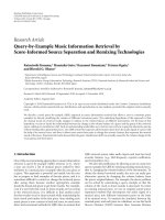
scenario are valid. As can be seen in Figure 1 the surveillance
system combines a detection unit and a tracking unit using a
method for determining and matching reliable objects based
on a projective transformation.
The aim of the detection unit is to detect moving
foreground regions and store the detection result in a binary
mask. A very common solution for moving foreground
detection is background subtraction. In background sub-
traction a reference background image is subtracted from

each frame of the sequence and binary masks with the
moving foreground objects are obtained by thresholding the
resulting difference images. The key problem in background
subtraction is to find a good background model. Commonly
a mixture of Gaussian distributions is used for modeling
the color values of a particular pixel over time [4–6].
Hence, the background can be modeled by a Gaussian
2 EURASIP Journal on Image and Video Processing
mixture model (GMM). Once the pixelwise GMM likelihood
is obtained, the final binary mask is either generated by
thresholding [4, 6, 7] or according to more sophisticated
decision rules [8–10]. Although the Gaussian mixture model
technique is quite successful, the obtained binary masks
are often noisy and irregular. The main reason for this is
that spatial and temporal dependencies are neglected in
most approaches. Thus, the method of our detection unit
improves the standard GMM method by regarding spatial
and temporal dependencies and integrating a limitation of
the standard deviation into the traditional method. While
the spatial dependency and the limitation of the standard
deviation lead to clear and noiseless object boundaries,
false positive detections caused by shadows and uncovered
background regions so called ghosts can be reduced due to
the consideration of the temporal dependency. By combining
this improved detection method with a fast shadow removal
technique, which is inspired by the technique of [3], the
quality of the detection result is further enhanced and good
binary masks are obtained without adding any complex and
computational expensive extensions to the method.
Once an object is detected and classified as reliable,

the actual tracking algorithm can be initialized. In [1]
tracking methods are divided into three main categories:
point tracking, kernel tacking, and silhouette tracking. Due
to its ease of implementation, computational speed, and
robust tracking performance, we decided to use a mean
shift-based tracking algorithm [11], which belongs to the
kernel tracking category. In spite of its advantages traditional
mean shift has two main drawbacks. The first problem is the
fixed scale of the kernel or the constant kernel bandwidth.
In order to achieve a reliable tracking result of an object
with changing size, an adaptive kernel scale is necessary.
Theseconddrawbackistheuseofaradialsymmetric
kernel. Since most objects are of anisotropic shapes, a
symmetric kernel with its isotropic shape is not a good
representation of the object shape. In fact if not specially
treated, the symmetric kernel shape may lead to an inclusion
of background information into the target model, which
can even cause tracking failures. An intuitive approach of
solving the first problem is to run the algorithm with three
different kernel bandwidths, former bandwidth and former
bandwidth
±10%, and to choose the kernel bandwidth which
maximizes the appearance similarity (
±10% method) [12].
A more sophisticated method using difference of Gaussian
mean shift kernel in scale space has been proposed in
[13]. The method provides good tracking results but is
computationally very expensive. And both methods are not
able to adapt to the orientation or the shape of the object.
Mean shift-based methods which are not only adapting

the kernel scale but also the orientation of the kernel
are presented in [14–17]. The method of [14] focuses on
face tracking and uses ellipses as basic face models; thus
it cannot easily be generalized for tracking other objects
since adequate models are required. Like in [15]scaleand
orientation of a kernel can be obtained by estimating the
second-order moments of the object silhouette, but that is
of high computational costs. In [16] mean shift is combined
with adaptive filtering to obtain kernel scale and orientation.
The estimations of kernel scale and orientation are good,
but since a symmetric kernel is used, no adaptation to the
actual object shape can be performed. Therefore, in [17]
asymmetric kernels are generated using implicit level set
functions. Since the search space is extended by a scale,
and an orientation dimension, the method simultaneously
estimates the new object position, scale, and orientation.
However the method can only estimate the objects orien-
tation for in-plane rotations. In case of 3D or out-of-plane
rotations none of the mentioned algorithms is able to adapt
to the shape of the object.
Therefore, for the tracking unit of Auto GMM-SAMT
we developed GMM-SAMT, a mean shift-based tracking
method which is able to adapt to the object contour no mat-
ter what kind of 3D rotation the object is performing. During
initialization the tracking unit generates an asymmetric and
shape-adapted kernel from the object mask delivered by the
previous units of Auto GMM-SAMT. During the tracking
the kernel scale is first adapted to the current object size
by running the mean shift iterations in an extended search
space. The scale-adapted kernel is then fully adapted to the

current contour of the object by a segmentation process
based on a maximum a posteriori estimation considering the
GMMs of the object and the background histogram. Thus, a
good fit of the object shape is retrieved even if the object is
performing out-of-plane rotations.
The paper is organzied as follows. In Section 2 the
detection of moving foreground regions is explained while
Section 3 describes the determination of reliable objects
among the detected foreground regions. GMM-SAMT, the
core of Auto GMM-SAMT, is presented in Section 4.The
whole system (Figure 1)isevaluatedinSection 5 and finally
conclusions are drawn in Section 6.
2. Moving Foreground Detection
2.1. GMM-Based Background Subtraction. As proposed in
[4] the probability of a certain pixel x in frame t having the
color value c is given by the weighted mixture of k
= 1 ···K
Gaussian distributions:
P
(
c
t
)
=
K

k=1
ω
k,t
·

1
(
2π
)
n/2
|Σ
k
|
1/2
e
(−1/2)(c−µ
k
)
T
Σ
−1
k
(c−µ
k
)
,
(1)
where c is the color vector and ω
k
the weight for the
respective Gaussian distribution. Σ is an n-by-n covariance
matrix of the form Σ
k
= σ
2

k
I, because it is assumed that the
RGB color channels have the same standard deviation and
are independent from each other. While the latter is certainly
not the case, by this assumption a costly matrix inversion can
be avoided at the expense of some accuracy. To update the
model for a new frame it is checked if the new pixel color
matches one of the existing K Gaussian distributions. A pixel
x with color c matches a Gaussian k if



c −µ
k



<d·σ
k
,(2)
EURASIP Journal on Image and Video Processing 3
Reliable
object
determination
Match
objects
New object
No
Ye s
Kernel

generation
from mask
Target model GMM-SAMT
Object contour
Object position
Monitor
Video signal
Shadow
removal
thresholding
for mask
generation
Background
model
Video signal
+
−
Camera
Figure 1: Auto GMM-SAMT: a video surveillance system for visual monitoring of traffic scenarios based on GMM-SAMT.
where d is a user-defined parameter. If c matches a distribu-
tion, the model parameters are adjusted as follows:
ω
k,t
=
(
1
−α
)
ω
k,t−1

+ α,
µ
k,t
=

1 −ρ
k,t

µ
k,t−1
+ ρ
k,t
c
t
,
σ
k,t
=


1 −ρ
k,t

σ
2
k,t
−1
+ ρ
k,t





c
t
−µ
k,t




2
,
(3)
where α is the learning rate and ρ
k,t
= α/ω
k,t
according to
[6]. For unmatched distributions only a new ω
k,t
has to be
computed following (4):
ω
k,t
=
(
1
−α
)

ω
k,t−1
.
(4)
The other parameters remain the same. The Gaussians
are now ordered by the value of the reliability measure
ω
k,t
/σ
k,t
in such a way that with increasing subscript k
the reliability decreases. If a pixel matches more than one
Gaussian distribution, the one with the highest reliability is
chosen. If the constraint in (2) is not fulfilled and a color
value cannot be assigned to any of the K distributions, the
least probable distribution is replaced by a distribution with
the current value as its mean value, a low prior weight, and
an initially high standard deviation and ω
k,t
is rescaled.
A color value is regarded to be background with higher
probability (lower k)ifitoccursfrequently(highω
k
)and
does not vary much (low σ
k
). To determine the B background
distributions a user-defined prior probability T is used:
B
= arg min

b
⎛
⎝
b

k=1
w
k
>T
⎞
⎠
. (5)
The rest K
−B distributions are foreground.
2.2. Temporal Dependency. The traditional method takes
into account only the mean temporal frequency of the color
values of the sequence. The more often a pixel has a certain
color value, the greater is the probability of occurrence
of the corresponding Gaussian distribution. But the direct
temporal dependency is not taken into account.
To detect the static background regions and to enhance
adaptation of the model to these regions, a parameter u is
introduced to measure the number of cases where the color
of a certain pixel was matched to the same distribution in
subsequent frames:
u
t
=
⎧
⎨

⎩
u
t−1
+1, ifk
t
= k
t−1
,
0, else,
(6)
where k
t−1
is the distribution which matched the pixel
color in the previous frame and k
t
is the current Gaussian
distribution. If u exceeds a threshold u
min
,thefactorα is
multiplied by a constant s>1:
α
t
=
⎧
⎨
⎩
α
0
·s,ifu
t

>u
min
,
α
0
,else.
(7)
The factor α
t
is now temporal dependent and α
0
is the
initial user-defined α. In regions with static image content
the model is now faster updated as background. Since the
method does not depend on the parameters σ and ω,the
detection is also ensured in uncovered regions. In the top row
of Figure 2 the original frame of sequence Parking
lot and
the corresponding background estimated using GMMs com-
bined with the proposed temporal dependency approach is
shown. The detection results of the standard GMM method
with different values of α are shown in the bottom row of
Figure 2. While the standard method detects a lot of either
false positives or false negatives, the method considering
temporal dependency obtains quite a good mask.
2.3. Spatial Dependency. In the standard GMM method, each
pixel is treated separately and spatial dependency between
adjacent pixels is not considered. Therefore, false positives
4 EURASIP Journal on Image and Video Processing
(a) (b)

(c) (d)
Figure 2: A frame of sequence Parking lot and the correspond-
ing detection results of the proposed method compared to the
traditional method. First row: original frame (a) and background
estimated by the proposed method with temporal dependency
(α
0
= 0.001, s = 10, u
min
= 15) (b). Bottom row: standard method
with α
= 0.001 (c) and α = 0.01 (d).
caused by noise-based exceedance of d · σ
k
in (2)orslight
lighting changes are obtained. Since the false positives of the
first type are small and isolated image regions, the ones of
the second type cover larger adjacent regions as they mostly
appear at the border of shadows, the so-called penumbra.
Through spatial dependency both kinds of false positives can
be eliminated.
Since in the case of false positives the color value c of
x is very close to the mean of one of the B distributions,
at least for one distribution k
∈ [1 ···B] a small value
is obtained for
|c − µ
k
|. In general this is not the case for
true foreground pixels. Instead of generating a binary mask

we create a mask M with weighted foreground pixels. For
each pixel x
= (x, y) its weighted mask value is estimated
according to the following equation:
M
(
x
)
=
⎧
⎪
⎨
⎪
⎩
0, if k
(
x
)
∈
[
1
···B
]
,
min
k=[1···B]





c −µ
k




,else.
(8)
The background pixels are still weighted with zero while the
foreground pixels are weighted according to the minimum
distance between the pixel and the mean of the background
distributions. Thus, foreground pixels with a larger distance
to the background distributions get a higher weight. To use
the spatial dependency as in [18], where the neighborhood
of each pixel is considered, the sum of the weights in a
square window W is computed. By using a threshold M
min
the number of false positives is reduced and a binary mask
BM is estimated from the weighted mask M according to
BM
(
x
)
=
⎧
⎪
⎨
⎪
⎩
1, if


W
M
(
x
)
>M
min
,
0, else.
(9)
(a) (b)
Figure 3: Detection result of the proposed method with temporal
dependency (a) compared to the proposed method with temporal
and spatial dependencies (b) for sequence Parking
lot (M
min
= 500
and W
= 5 ×5).
0
10
20
30
40
50
60
Standard deviation σ
20 40 60 80 100 120 140
Frame number

σ
max
σ
mean
σ
min
σ
0
Figure 4: Maximum, mean, and minimum standard deviation of
all Gaussian distribution of all pixels for the first 150 frames of
sequence Street.
In Figure 3(b) part of a binary mask for sequence
Parking
lot obtained by GMM method considering temporal
as well as spatial dependency is shown.
2.4. Background Quality Enhancement. If a pixel in a new
frame is not described very well by the current model, the
standard deviation of a Gaussian distribution modelling the
foreground might increase enourmously. This happens most
notably when the pixel’s color value deviates tremendously
from the mean of the distribution and large values of c
−
µ
k
are obtained during the model update. The larger σ
k
gets, the more color values can be matched to the Gaussian
distribution. Again this increases the probability of large
values of c
−µ

k
.
Figure 4 illustrates the changes of the standard deviation
over time for the first 150 frames of sequence Street modeled
by 3 Gaussians. The minimum, mean, and maximum
standard deviations of all Gaussian distributions for all
pixels are shown (dashed lines). The maximum standard
deviation increases over time and reaches high values. Hence,
all pixels which are not assigned to one of the other two
distributions will be matched to the distribution with the
large σ value. The probability of occurrence increases and
EURASIP Journal on Image and Video Processing 5
(a) (b)
Figure 5: Background estimated for sequence Street without (a)
and with limited standard deviation σ
0
= 10 (b). Ellipse marks
region, where detection artefacts are very likely to occur.
the distribution k will be considered as a background
distribution. Therefore, even foreground colors are easily but
falsely identified as background colors. Thus, we suggest to
limit the standard deviation to the initial standard deviation
value σ
0
as demonstrated in Figure 4 by the continuous red
line. In Figure 5 the traditional method (left background)
is compared to the one where the standard deviation is
restricted to the initial value σ
0
= 10 (right background). By

examining the two backgrounds it is clearly visible that the
limitation of the standard deviation improves the quality of
the background model, as the dark dots and regions in the
left background are not contained in the right background.
2.5. Single Step Shadow Removal. Even though the consid-
eration of spatial dependency can avert the detection of
most penumbra pixels, the pixels of the deepest shadow,
the so-called umbra, might still be detected as foreground
objects. Thus, we combined our detection method with a
fast shadow removal scheme inspired by the method of [3].
Since a shadow has no affect on the hue but changes the
saturation and decreases the luminance, possible shadow
pixels can be determined as follows. To find the true shadow
pixels, the luminance change h is determined in the RGB
space by projecting the color vector c onto the background
color value b. The projection can be written as h
=

c, b/|b|. A luminance ratio is defined as r =|b|/h to
measure the luminance difference between b and c while the
angle φ
= arccos(h/c) between the color vector c and the
background color value b measures the saturation difference.
Each foreground pixel is classified as a shadow pixel if the
following two terms are both statisfied:
r
1
<r<r
2
, φ<

φ
2
−φ
1
r
2
−r
1
·
(
r
−r
1
)
+ φ
1
, (10)
where r
1
is the maximum allowed darkness, r
2
is the
maximum allowed brightness, and φ
1
and φ
2
are the max-
imum allowed angle separation for penumbra and umbra.
Compared to the shadow removal scheme described in [3],
the proposed technique supresses penumbra and umbra

simultaneously while the method of [3]hastoberuntwice.
More details can be found in [19].
3. Determination of Reliable Objects
After the GMM-based background subtraction it has to be
decided which of the detected foreground pixels in the binary
mask represent true and reliable object regions. In spite of
its good performance the background subtraction unit still
needs a few frames to adjust when an object, which has not
been moving for a long time, suddenly starts to move. During
this period uncovered background regions, also referred to as
ghosts,canbedetectedasforeground.Toavoidatrackingof
these wrong detection results we have to distinguish between
reliable (true objects) and nonreliable objects (uncovered
background). Since it does not make sense to track objects
which only appear in the scene for a few frames, these objects
are also considered as nonreliabel objects.
The unit for determining reliable objects among the
detected foreground regions consists mainly of a connected
component analysis (CCA) and a matching process, which
performs a projective transformation to be able to incor-
porate the size information as a useful matching criterion.
Connected component analysis (CCA) is applied on the
binary masks to determine connected foreground regions, to
fill small holes of the foreground regions, and to compute
the centroid of each detected foreground region. CCA can
also be used to compute the area size of each foreground
region. In general size is an important feature to descriminate
different objects. But since the size of moving objects changes
while the object moves towards or away from the camera,
the size information obtained from the binary masks is not

very useful. Especially in video surveillance systems which
are operating with low frame rates like 3 to 5 fps the size
of a moving object might change drastically. Therefore, we
transform the binary masks as if they were estimated from a
sequence which has been recorded by a camera with top view.
Figure 6 shows the original and the transformed versions of
two images and their corresponding binary masks.
According to a projective transformation each pixel x
1,i
oftheoriginalviewisprojectedontotheimageplaneofa
virtual camera with a top view of the recorded scene. The
direct link between a pixel x
1,i
in the original camera plane
I
1
and its corresponding pixel x
2,i
= [x
2,i
, y
2,i
, w
2,i
]
T
in the
camera plane of the virtual camera is given by
x
2,i

= H ·x
1,i
=
⎡
⎢
⎢
⎢
⎣
h
T
1
·x
1,i
h
T
2
·x
1,i
h
T
3
·x
1,i
⎤
⎥
⎥
⎥
⎦
, (11)
where H is the transformation or homography matrix and h

T
j
is the jth row of H . To perform the projective transformation
which is also called homography the according homography
matrix H is needed. The homography matrix can be
estimated either based on extrinsic and intrinsic camera
parameters and three point correspondences or based on
at least four point correpondences. We worked with point
correspondences only, which were chosen manually between
one frame of the surveillance sequence and a satellite imagery
6 EURASIP Journal on Image and Video Processing
(a)
(b)
Figure 6: Original frames and binary masks of sequence Airport (a) and the transformed versions (b). In the orginial binary masks the object
size changes according to the movement of the objects, while in the transformed binary masks the object sizes stay more or less constant and
the ratio of the object sizes is kept.
of the scene. By estimating the vector product x
2,i
× H · x
1,i
and regarding that h
T
j
· x
1,i
= x
T
1,i
· h
j

we get a system of
equations of the form A
i
h = 0,whereA
i
is a 3×9matrixand
h
= (h
1
, h
2
, h
3
)
T
;see[20] for details. Since only two linear
independent equations exist in A
i
, A
i
can be reduced to a 2×9
matrix and the following equation is obtained:
A
i
h=
⎡
⎣
0
T
−w

2,i
·x
1,i
y
2,i
·x
1,i
w
2,i
·x
1,i
0
T
−x
2,i
·x
1,i
⎤
⎦
⎡
⎢
⎢
⎢
⎣
h
T
1
h
T
2

h
T
3
⎤
⎥
⎥
⎥
⎦
=
0. (12)
If four point correspondences are known, the matrix H can
be estimated from (12) except for a scaling factor. To avoid
the trivial solution the scaling factor is set to the norm
h=1. Since in our case always more than four point
correspondences are known, one can again use the norm
h=1 as an additional condition and use the basic direct
linear transformation (DLT) algorithm [20] for estimating
H or the set of equations in (12) has to be turned into an
inhomogeneous set of linear equations. For the latter one
entry of h has to be chosen such that h
j
= 1. For example,
with h
9
= 1 we obtain the following equations from (12):
⎡
⎣
000−x
1,i
w

2,i
−y
1,i
w
2,i
−w
1,i
w
2,i
x
1,i
y
2,i
y
1,i
y
2,i
x
1,i
w
2,i
y
1,i
w
2,i
w
1,i
w
2,i
000−x

1,i
x
2,i
−y
1,i
x
2,i
⎤
⎦

h =
⎛
⎝
−
w
1,i
y
2,i
w
1,i
x
2,i
⎞
⎠
, (13)
EURASIP Journal on Image and Video Processing 7
where

h is an 8-dimensional vector consisting of the first 8
elements of h. Concatenating the equations from more than

four point correspondences a linear set of equations of the
form of M

h = b is obtained which can be solved by a least
squares technique.
In case of airport apron surveillance or other surveillance
scenarios where the scene is captured from a (slanted) top
view position, moving objects on the ground can be con-
sidered as flat compared to the reference plane. Thus, in the
transformed binary masks the size of the detected foreground
regions almost does not change over the sequence, compare
masks in Figure 6.Hence,wecannowusethesizefor
detecting reliable objects. Since airplanes and vehicles are the
most interesting objects on the airport apron, we only keep
detected regions which are bigger than a certain size A
min
in
the transformed binary image. In most cases A
min
can also
be used to distinguish between airplanes and other vehicles.
After removing all foreground regions which are smaller than
A
min
, the binary mask is transformed back into the original
view. All remaining foreground regions in two subsequent
frames are then matched by estimating the shortest distance
between the centroids. We define a foreground region as a
reliable object, if the region is detected and matched in n
= 5

subsequent frames.
The detection result of a reliable object already being
tracked is compared to the tracking result of GMM-SAMT
to check if the detection result is still valid; see Figure 1.
The comparison is also used as a final refinement step
for the GMM-SAMT results. In case of very similar object
and background color the tracking result might miss small
object segments at the border of the object, which might be
identified as object regions during the detection step and can
be added to the object shape. Also small object segments
at the border of the object, which are actually background
regions, can be identified and corrected by comparing the
tracking result with the detection result. For objects, which
are considered as realiable for the first time, the mask of
the object is used to build the shape adaptive kernel and
to estimate the color histogram of the object for generating
the target model as described in Sections 4.1 and 4.2.After
the adaptive kernel and target model are estimated, GMM-
SAMT can be initialized.
4. Object Tracking Using GMM-SAMT
4.1. Mean Shift Tracking Overview. Mean shift tracking
discriminates between a target model in frame n and a
candidate model in frame n+1. The target model is estimated
from the discrete density of the objects color histogram
q(
x) ={q
u
(x)}
u=1···m
(whereas


m
u
=1
q
u
(x) = 1). The
probability of a certain color belonging to the object with
the centroid
x is expressed as q
u
(x), which is the probability
of the feature u
= 1 ···m occuring in the target model.
The candidate model p(
x
new
) is defined analogous to the
target model; for more details see [21, 22]. The core of the
mean shift method is the computation of the offset from an
old object position
x to a new position x
new
= x + Δx by
(a) (b)
0
0.5
1
(c)
Figure 7: Object in image (a), object mask (b), and asymmetric

object kernel retrieved from object mask (c).
estimating the mean shift vector:
Δx
=

i
K
(
x
i
− x
)
ω
(
x
i
)(
x
i
− x
)

i
K
(
x
i
− x
)
ω

(
x
i
)
,
(14)
where K(
·) is a symmetric kernel with bandwidth h defining
the object area and ω(x
i
) is the weight of x
i
which is defined
as
ω
(
x
i
)
=
m

u=1
δ
[
b
(
x
i
)

−u
]



q
u
(
x
)
p
u
(
x
new
)
,
(15)
where b(
·) is the histogram bin index function and δ(·)
is the impulse function. The similarity between target and
candidate model is measured by the discrete formulation of
the Bhattacharya coefficient:
ρ

p
(
x
new
)

, q
(
x
)

=
m

u=1

p
u
(
x
new
)
q
u
(
x
)
.
(16)
The aim is to minimize the distance between the two color
distributions d(
x
new
) =

1 −ρ[p(x

new
), q(x)] as a function
of
x
new
in the neighborhood of a given position x
0
.This
can be achieved using the mean shift algorithm. By running
this algorithm the kernel is recursively moved from
x
0
to x
1
according to the mean shift vector.
4.2. Asymmetric Kernel Selection. Standard mean shift track-
ing is working with a symmetric kernel. But an object
shape cannot be described properly by a symmetric kernel.
Therefore, the use of isotropic or symmetric kernels will
always cause an influence of background information on the
target model, which can even lead to tracking errors. To
overcome these difficulties we are using an asymmetric and
anisotropic kernel [17, 21, 23]. Based on the object mask
generated by the detection unit of Auto GMM-SAMT an
asymmetric kernel is constructed by estimating for each pixel
8 EURASIP Journal on Image and Video Processing
0
0.018
p(c
g

)
0 100 200
c
g
(a)
0
0.018
p(c
g
)
0 100 200
c
g
(b)
Figure 8: Modeling the histogram of the green color channel of the car in sequence Parking lot with K = 5 (a) and K = 8 Gaussians (b).
inside the mask x
i
= (x, y) its normalized distance to the
object boundary:
K
s
(
x
i
)
=
d
(
x
i

)
d
max
, (17)
where the distance from the boundary is estimated by
iteratively eroding the outer boundary of the object shape
and adding the remaining object area to the former object
area. In Figure 7 an object, its mask, and the mask-based
asymmetric kernel are shown.
4.3. Mean Shift Tracking in Spat ial-Scale-Space. Instead of
running the algorithm only in the local space the mean shift
iterations are performed in an extended search space Ω
=
(x, y, σ) consisting of the image coordinates (x, y)andascale
dimension σ as described in [17]. Thus, the object’s changes
in position and scale can be evaluated through the mean shift
iterations simultaneously. To run the mean shift iterations in
the joint search space a 3D kernel consisting of the product of
the spatial object-based kernel from Section 4.2 and a kernel
for the scale dimension
K

x, y, σ
i

=
K

x, y


K
(
σ
)
(18)
is defined. The kernel for the scale dimension is a 1D
Epanechnikov kernel with the kernel profile k(z)
= 1 −|z|
if |z| < 1and0otherwise,wherez = (σ
i
− σ)/h
σ
.Themean
shift vector given in (14) can now be computed in the joint
space as
ΔΩ
=

i
K

Ω
i
−

Ω

ω
(
x

i
)

Ω
i
−

Ω


i
K

Ω
i
−

Ω

ω
(
x
i
)
(19)
with ΔΩ
= (Δx, Δy, Δσ), where Δσ is the scale update.
Given the object mask for the initial frame the object
centroid
x and the target model are computed. To make

the target model more robust the histogram of a specified
neighborhood of the object is also estimated and bins of
the neighborhood histogram are set to zero in the target
histogram to eliminate the influence of colors which are
contained in the object as well as in the background. In
case of an object mask with a slightly different shape than
the object shape too many object colors might be supressed
in the target model, if the direct neighbored pixels are
considered. Therefore, the directly neighbored pixels are not
included in the considered neighborhood. The mean shift
iterations are then performed as described in [17, 23]and
the new position of the object as well as a scaled object shape
will be determined, where the latter can be considered as a
first shape estimate.
4.4. Shape Adaptation Using GMMs. After the mean shift
iterations have converged, the final shape of the object is
evaluated from the first estimate of the scaled object shape.
Thus, the image is segmented using the mean shift method
according to [22]. For each segment being only partly
included in the found object area we have to decide if it still
belongs to the object shape or to the background. Therefore,
we learn two Gaussian mixture models, one modeling the
color histogram of the background and one the histogram
of the object. The GMMs are learned at the beginning of
the tracking based on the corresponding object binary mask.
Since we are working in RGB color space, the multivariate
normal density distribution of a color value c
= (c
r
, c

g
, c
b
)
T
is given by
p

c | µ
k
, Σ
k

=
1
(
2π
)
3/2
|Σ
k
|
1/2
e
−(1/2)(c−µ
k
)
T
Σ
−1

k
(c−µ
k
)
,
(20)
where µ
k
is the mean and Σ is a 3 ×3 covariance matrix. The
Gaussian mixture model for an image area is given by
P
(
c
)
=
K

k=1
P
k
· p

c | µ
k
, Σ
k

,
(21)
where P

k
is the a priori probability of distribution k,which
can also be interpreted as the weight for the respective
Gaussian distribution. To fit the Gaussians of the mixture
model to the corresponding color histogram the parameters
EURASIP Journal on Image and Video Processing 9
Table 1: Recall and Precision and F
1
measure of standard GMM and of improved GMM method of the Auto GMM-SAMT detection unit.
Sequence Ground truth frames
Standard GMM Detection unit of Auto GMM-SAMT
Recall Precision F
1
score Recall Precision F
1
score ΔF
1
Parking lot 30 0.91 0.47 0.62 0.95 0.77 0.85 0.23
Shopping
mall 20 0.88 0.47 0.62 0.83 0.77 0.80 0.18
Airport
hall 20 0.67 0.53 0.60 0.70 0.67 0.68 0.08
Airport 15 0.57 0.24 0.34 0.60 0.33 0.43 0.09
PETS 2000 15 0.99 0.45 0.61 0.99 0.72 0.83 0.22
(a)
(b)
Figure 9: Input frame, ground truth, and detection results of standard GMM method and of the Auto GMM-SAMT detection unit are
shown from left to right for sequence Shopping
Mall (a) and for sequence Airport Hall (b).
Θ

k
={P
k
, μ
k
, Σ
k
} are estimated using the expectation max-
imization (EM) algorithm [24]. During the EM iterations,
first the probability (at iteration step t)ofallN data samples
c
n
to belong to the kth Gaussian distribution is calculated by
Bayes’ theorem:
p
(
k
| c
n
, Θ
)
=
P
k,t
p

c
n
| k, µ
k,t

, Σ
k,t


K
k
=1
P
k,t
p

c
n
| k, µ
k,t
, Σ
k,t

, (22)
which is known as the expectation step. In the subsequent
maximization step the likelihood of the complete data is
maximized by re-estimating the parameters Θ:
P
k,t+1
=
1
N
N

n=1

p
(
k | c
n
, Θ
)
,
µ
k,t+1
=
1
NP
k,t+1
N

n=1
p
(
k | c
n
, Θ
)
c
n
,
Σ
k,t+1
=
1
NP

k,t+1
N

n=1
p
(
k | c
n
, Θ
)

c
n
−μ
t+1

c
n
−μ
t+1

T
.
(23)
The updated parameter set is then used in the next iteration
step t +1. The EM algorithm iterates between these two steps
and converges to a local maximum of the likelihood. Thus,
after convergence the GMM will be fitted to the discrete
data giving a nice representation of the histogram; see
Figure 8. Since the visualization of a GMM modeling a three-

dimensional histogram is rather difficult to understand,
Figure 8 shows two GMMs modeling only the histogram of
the green color channel of the car in sequence Parking
lot.
The accuracy of a GMM depends on the number of Gaus-
sians. Hence, the GMM with K
= 8 Gaussian distributions
models the histogram more accurate than the model with
K
= 5 Gaussians. Of course, depending on the histogram
in some cases a GMM with a higher number of Gaussian
distributions might be necessary, but for our purpose a
GMM with K
= 5 Gaussians showed to be a good trade-off
between modeling accuracy and parameter estimation.
To decide for each pixel if it belongs to the GMM of
the object P
obj
(c) = P(c | α = 1) or to the background
GMM P
bg
(c) = P(c | α = 0) we use maximum a posteriori
(MAP) estimation. Using log-likelihoods the typical form of
the MAP estimate is given by
α = arg max
α

ln p
(
α

)
+lnP
(
c | α
)

,
(24)
10 EURASIP Journal on Image and Video Processing
(a)
(b)
(c)
Figure 10: Input frame, ground truth, and detection results of standard GMM method and of the Auto GMM-SAMT detection unit are
shown from left to right for sequences Parking
lot (a), Airport (b), and PETS 2000 (c).
Table 2: Learning rate and shadow removal parameters.
Scenario α
0
r
1
r
2
φ
1
φ
2
Indoor 0.002 1 2.3 1 4
Outdoor 0.001 1 1.7 4 6
where α ∈ [0, 1] indicates that a pixel, or more precise
its color value c, belongs to the object (

α = 1) or the
background class (
α = 0), and p(α)isthecorrespondinga
priori probability. To set p(α) to an appropriate value object
and background area of the initial mask are considered.
Based on the number of its object and background
pixels, a segment is assigned as an object or background
segment. If more than 50% of the pixels of a segment belong
to the object class, the segment is assigned as an object
segment; otherwise the segment is considered to belong to
the background. The tracking result is then compared to the
according detection result of the GMM-based background
subtraction method. Segments of the GMM-SAMT result,
which match the detected moving foreground region, are
considered as true moving object segments. But segments
which are not at least partly included in the moving
foreground region of the background subtraction result are
discarded, since they are most likely wrongly assigned as
object segments due to errors in the MAP estimation caused
by very similar foreground and background colors. Hence,
the final object shape consists only of segments complying
with the constraints of the background subtraction as well
as the constraints of the GMM-SAMT procedure. Thus, we
obtain quite a trustworthy representation of the final object
shape from which the next object-based kernel is generated.
Finally, the next mean shift iterations of GMM-SAMT can be
initialiezed.
5. Exp erimental Results
The performance of Auto GMM-SAMT was tested on
several sequences showing typical traffic scenarios recorded

outside. To show that the detection method itself is also
applicable for other surveillance scenarios, it was also tested
on indoor surveillance sequences. In particular, the detection
method was tested on two indoor sequences provided by
[9] and three outdoor sequences, while the tracking and
overall performance of Auto GMM-SAMT was tested on five
outdoor sequences. For each sequence at least 15 ground
truth frames were either manually labeled or taken from [9].
Overall the performance of Auto GMM-SAMT was evaluated
on a total of 200 sample frames.
After parameter testing the GMM methods achieved
good detection results for all sequences with K
= 3
Gaussians, T
= 0.7, d = 2.5, and σ
0
= 10, whereas the
parameters for temporal dependency u
min
= 15 and s = 10
and for spatial dependency were set to M
min
= 500 and
W
= 5 ×5. Due to the very different illumination conditions
in the indoor and outdoor scenarios, the learning rate α
0
and
the shadow removal parameters were chosen separately for
indoor sequences and outdoor sequences; see Ta b l e 2 .

Detection results for the indoor sequences Shopping
Mall
and Ai rport
Hall can be seen in Figure 9 while detection
EURASIP Journal on Image and Video Processing 11
Figure 11: Mask of a car in sequence Parking lot generated by the Auto GMM-SAMT detection unit, mask after removing foreground
regions of uninteresting size, initialization of the Auto GMM-SAMT tracking unit for tracking the car, and the corresponding tracking result
for the next frame (shown from left to right).
(a)
(b)
Figure 12: Tracking results of Auto GMM-SAMT for sequence Parking lot (a) and for sequence PETS 2000 (b).
results for outdoor scenarios are shown in Figure 10.In
particular, the images shown from left to right in each
row of Figure 9 and of Figure 10 are the input frame, the
ground truth, the standard GMM result, and the result
of the Auto GMM-SAMT detection unit. By comparing
the results, one can clearly see that for both scenarios
the detection unit of Auto GMM-SAMT achieves much
better binary masks than the standard GMM method. To
further evaluate the detection performance the information
retrieval measurements Recall and Precision were computed
by comparing the detection results to the ground truth as
follows:
Recall
=
Number of correctly detected object pixels
Number of object pixels in the ground truth
,
Precision
=

Number of correctly detected object pixels
Number of all detected pixels
.
(25)
For sequences Shopping
Mall and Airport Hall the ground
truths of [9] were taken, while for all other sequences
the ground truths were manually labeled. The Recall and
Precision scores given in Tab l e 1 confirm the impression of
the visual inspection, since for all test sequences the detection
unit of Auto GMM-SAMT achieves better results as the
standard GMM method. In addition to the information
retrieval measurements, we also calculated the even more
significant F
1
measure:
F
1
= 2 ·
Recall · Precision
Recall + Precision
.
(26)
Again the visual impression is confirmed. The F
1
scores of
the standard GMM method and of the Auto GMM-SAMT
detection unit are compared in the last column of Tab l e 1.
To determine reliable objects among the detected fore-
ground regions the obtained binary masks are transformed

using the corresponding homography matrix. The homog-
raphy matrix is estimated only once at the beginning of a
sequence and can then be used for the whole sequence. A
recalculation of the homography matrix is not necessary.
Thus, the homography estimation can be considered as a
calibration step of the surveillance system, which does not
influence the computational performance of Auto GMM-
SAMT at all. In the transformed mask only foreground
regions of interesting size A (e.g., A
≥ A
min
)arekeptand
considered as possible object regions. For our purpose A
min
was set to 2000 pixels for detecting cars and to 75000 pixels
for airplanes.
After possible object regions are estimated in the trans-
formed binary mask, the mask is transformed back into the
original view. All possible object regions, which could be
matched in n
= 5 subsequent frames, are considered as
reliabel objects. For each reliable detected object the masked-
based kernel is generated. Each object kernel is then used for
12 EURASIP Journal on Image and Video Processing
(a)
(b)
Figure 13: Tracking results using the standard mean shift tracker combined with the ±10% method (The result of the standard mean
shift tracker indicated by the red dotted ellipses is hard to see. Can you please enhance the visibility of the red dotted ellipses?) and Auto
GMM-SAMT (green solid contour) for tracking an airplane and a car in sequences Airplane (a) and F ollow
me (b), respectively.

Table 3: Recall and Precision and F
1
measure of standard mean shift tracking and GMM-SAMT.
Sequence Ground truth frames
Standard mean shift GMM-SAMT
t
err
Recall Precision F
1
score t
err
Recall Precision F
1
score ΔF
1
Parking 30 9 0.96 0.52 0.68 3 0.98 0.86 0.92 0.24
Follow
me 20 88 0.23 0.14 0.60 3 0.99 0.83 0.90 0.30
Airplane 20 11 0.33 0.77 0.46 8 0.63 0.81 0.71 0.25
Airport 15 32 0.75 0.25 0.37 4 0.84 0.76 0.80 0.43
PETS 2000 15 8 0.80 0.79 0.80 1 0.97 0.91 0.94 0.14
computing the weighted histogram in the RGB space with
32
×32 ×32 bins. For the scale dimension the Epanechnikov
kernel with a bandwidth of h
σ
= 0.4isused.Formeanshift
segmentation a multivariate kernel defined according to (35)
in [22] as the product of two Epanechnikov kernels, one for
the spatial domain (pixel coordinates) and one for the range

domain (color), is used. The bandwidth of the Epanechnikov
kernel in range domain was set to h
r
= 4, and the bandwidth
of the one in spatial domain to h
s
= 5. The minimal segment
size was set to 5 pixels. Since the colors of an object and the
surrounding background do not change to drastically in the
considered scenarios, while the object is being tracked, the
object and background GMMs for the MAP decision are only
estimated at the beginning of the tracking by running the
EM algorithm until convergence or for a maximum number
of 30 iterations. Since Auto GMM-SAMT is developed for
video surveillance of traffic scenarios, which are recorded
diagonally from above such that the homography leads to
reasonable results, the tracking performance was tested on
five outdoor sequences containing mainly three-dimensional
rigid objects.
In Figure 11 the performance of Auto-GMM-SAMT
after initialization with a suboptimal object mask is illus-
trated. The first two images in Figure 11 show a binary
mask for sequence Parking
lot before and after removing
foreground regions of uninteresting size, while the initial-
ization of the Auto GMM-SAMT tracking unit using the
refined mask is given in the third image. The tracking
result for the subsequent frame of sequence Parking
lot
is provided in the fourth image of Figure 11.Despite

the uncovered background contained in the initializa-
tion mask, Auto GMM-SAMT immediately recovers from
this weak initialization. More tracking results of Auto
GMM-SAMT for sequences Parking
lot and PETS 2000
( can be seen in
Figure 12. In both cases Auto GMM-SAMT is able to track
the contour of the cars, even though the cars are performing
out-of-plane rotations.
In Figure 13 the tracking results of Auto GMM-SAMT
(green solid contour) are compared to the results of the
standard mean shift tracker combined with the
±10%
method (red dotted ellipse). While Auto GMM-SAMT is able
to adapt to the shape of the turning airplane, the standard
method even fails to fit the scale and the position of the
ellipse to the size and location of the airplane; see top row
of Figure 13. Beside that, standard mean shift tracking also
tends to track only a part of the object. This typical behaviour
of the standard mean shift can even lead to tracking failure
as, for instance, in the case of the turning car in sequence
Follow
me (bottom row of Figure 13).
The visual evaluation of the tracking results already
shows that Auto GMM-SAMT clearly outperforms the
standard mean shift algorithm. To further evaluate the
tracking result the tracking error t
err
in pixels is estimated
by computing the averaged euclidean distance of the tracked

centroids to the ground truth centroids, see Tables 3 and 4.
EURASIP Journal on Image and Video Processing 13
Table 4: Recall, Precision, and F
1
score of Auto GMM-SAMT.
Sequence Ground truth frames
Auto GMM-SAMT ΔF
1
compared to
t
err
Recall Precision F
1
score Standard mean shift GMM-SAMT
Parking lot 35 3 0.99 0.83 0.90 0.22 −0.02
Follow
me 20 2 0.99 0.86 0.92 0.32 0.02
Airplane 20 3 0.91 0.78 0.84 0.38 0.13
Airport 15 4 0.88 0.75 0.81 0.44 0.01
PETS 2000 15 3 0.98 0.86 0.92 0.12
−0.02
Since the standard method failes to track the follow-me car,
the tracking error is extremly high in that case and does
not represent the general performance of the standard mean
shift tracker. However, GMM-SAMT and Auto GMM-SAMT
also outperform the standard mean shift tracking in all other
cases. Recall and Precision as well as the F
1
measure were
also computed for the tracking results by comparing the

number of (correctly) tracked object pixels to the tracking
ground truths. The Recall and Precision scores confirm the
impression of the visual inspection since for all test sequences
Auto GMM-SAMT exceeds the standard mean shift method;
see Tables 3 and 4. By taking a look at the F
1
scores in
Ta b l e s 3 and 4, one also recognizes that Auto GMM-SAMT
keeps up with the stand alone implementation of GMM-
SAMT. This is indeed quite a nice matter of fact, since the
stand alone GMM-SAMT is initialized by the user with very
precise initial masks, while the automatic estimated masks
of the Auto GMM-SAMT detection unit are likely to be less
precise; compare Figure 11. Despite Auto GMM-SAMT does
not suffer from a loss of quality, for some sequences Auto
GMM-SAMT achieves even higher F
1
scores.
The performance of the detection unit (implemented in
C++) is about 29 fps for 480
× 270 image resolution on a
2.83 GHz Intel Core 2 Q9550. By using multithreading the
performance is further enhanced up to 60.16 fps using 4
threads. Since the tracking unit is implemented in Matlab,
it does not perform in real-time yet. But our modifications
do not add any computational expensive routines to the
mean shift method and the EM-algorithm is only run at
the beginning of the tracking. Thus, a good computational
performance should also be possible for a C/C++ implemen-
tation of the tracking unit.

6. Conclusions
The presented Auto GMM-SAMT video surveillance system
shows that the GMM-SAMT algorithm could succesfully
be combined with our improved GMM-based background
subtraction method. Thus, an automatic object tracking for
video surveillance is achieved.
On the one hand Auto GMM-SAMT takes adavantage
of GMM-SAMT, which extends the standard mean shift
algorithm to track the contour of objects of changing shape
without the help of any predefined shape model. Since
the tracking unit works with object mask-based kernels,
the influence of background colors on the target model is
avoided. Thus, the Auto GMM-SAMT tracking unit is much
more robust than standard mean shift tracking. Because of
adapting the kernel to the current object shape in each frame,
Auto GMM-SAMT is able to track the shape of an object even
if the object is performing out-of-plane rotations.
On the other hand Auto GMM-SAMT automates the
initialization of the tracking algorithm using our improved
GMM-based detection algorithm. Because of the limitation
of the standard deviation and the consideration of temporal
and spatial dependencies in the detection unit, the Auto
GMM-SAMT system obtains good binary masks. Even
uncovered background regions are relatively fast classified
as background due to the spatiotemporal adaptive detec-
tion method. Despite this fast adaptation to uncovered
background areas, for a few frames false positives caused
by uncovered background regions might be contained in
the masks. But it is shown that the GMM-SAMT track-
ing method can also achieve good tracking result when

initialized with binary masks of moderate quality as long
as the color of object and (uncovered) background is not
too similar. Otherwise Auto GMM-SAMT will deliver the
first correct object contours after the uncovered background
is correctly identified as such by the detection unit. Nev-
ertheless, Auto GMM-SAMT can keep up with the stand
alone implementation of GMM-SAMT. In some cases Auto
GMM-SAMT performs even better than GMM-SAMT due
to the final shape refinement when comparing the tracking
results with the background subtraction results. However, in
the case of very similar foreground and background colors
detection and tracking problems can occur.
In addition, the projective transformation of Auto
GMM-SAMT can be considered only as a fast but very simple
object classification. Since the classification is not reliable
enough for a robust surveillance system, we will focus on
otherobjectfeaturesaswellasonalternativeclassification
techniques in our future work. The consideration of other
object features could also help to improve the detection
and tracking performance in case of very similar object and
background colors. Besides we also plan to investigate the
automation of the homography estimation to remove the
manual calibration step.
Acknowledgments
This work has been supported by Gesellschaft f
¨
ur Informatik,
Automatisierung und Datenverarbeitung (iAd) and the Bun-
desministerium f
¨

ur Wirtschaft und Technologie (BMWi), ID
20V0801I.
14 EURASIP Journal on Image and Video Processing
References
[1] A.Yilmaz,O.Javed,andM.Shah,“Objecttracking:asurvey,”
ACM Computing Surveys, vol. 38, no. 4, pp. 1–45, 2006.
[2]M.Borg,D.Thirde,J.Ferrymanetal.,“Videosurveillance
for aircraft activity monitoring,” in Proceedings of the IEEE
International Conference on Advanced Video and Signal-Based
Surveillance (AV SS ’05), pp. 16–21, Como, Italy, 2005.
[3]F.PorikliandO.Tuzel,“Humanbodytrackingbyadaptive
background models and mean-shift analysis,” in Proceedings
of the IEEE International Workshop on Performance Evaluation
of Tracking and Surveillance (PETS-ICVS ’03), Graz, Austria,
2003.
[4] C. StaufferandW.E.L.Grimson,“Adaptivebackground
mixture models for real-time tracking,” in Proceedings of the
IEEE Computer Society Conference on Computer Vision and
Pattern Recognition (CVPR ’99), vol. 2, pp. 252–258, Miami,
Fla, USA, 1999.
[5] C. Stauffer and W. E. L. Grimson, “Learning patterns of
activity using real-time tracking,” IEEE Transactions on Pattern
Analysis and Machine Intelligence, vol. 22, no. 8, pp. 747–757,
2000.
[6] P.W.PowerandJ.A.Schoonees,“Understandingbackground
mixture models for foreground segmentation,” in Proceedings
of the Image and Vision Computing (IVCNZ ’02), pp. 267–271,
Auckland, New Zealand, November 2002.
[7] P. KaewTraKulPong and R. Bowden, “An improved adap-
tive background mixture model for real-time tracking with

shadow detection,” in Proceedings of the 2nd European Work-
shop Advanced Video Based Surveillance Systems (AVBS ’01),
vol. 1, Kingston upon Thames, UK, 2001.
[8] L. Carminati and J. Benois-Pineau, “Gaussian mixture classifi-
cation for moving object detection in video surveillance envi-
ronment,” in Proceedings of the IEEE International Conference
on Image Processing (ICIP ’05), vol. 3, pp. 113–116, Genoa,
Italy, 2005.
[9] L. Li, W. Huang, I. Y H. Gu, and Q. Tian, “Statistical modeling
of complex backgrounds for foreground object detection,”
IEEE Transactions on Image Processing, vol. 13, no. 11, pp.
1459–1472, 2004.
[10] S. Y. Yang and C. T. Hsu, “Background modeling from gmm
likelihood combined with spatial and color coherency,” in
Proceedings of the IEEE International Conference on Image
Processing (ICIP ’06), pp. 2801–2804, Atlanta, Ga, USA, 2006.
[11] D. Comaniciu, V. Ramesh, and P. Meer, “Real-time tracking
of non-rigid objects using mean shift,” in Proceedings of the
IEEE Conference on Computer Vision and Pattern Recognition,
pp. 142–149, Hilton Head, SC, USA, 2000.
[12] D. Comaniciu, V. Ramesh, and P. Meer, “Kernel-based object
tracking,” IEEE Transactions on Pattern Analysis and Machine
Intelligence, vol. 25, no. 5, pp. 564–577, 2003.
[13] R. T. Collins, “Mean-shift blob tracking through scale space,”
in Proceedings of the IEEE Conference on Computer Vision and
Pattern Recognition (CVPR ’03), vol. 2, pp. 234–240, Madison,
Wis, USA, 2003.
[14] V. Vilaplana and F. Marques, “Region-based mean shift
tracking: application to face tracking,” in Proceedings of the
15th IEEE International Conference on Image Processing (ICIP

’08), pp. 2712–2715, San Diego, Calif, USA, 2008.
[15] G. R. Bradski, “Computer vision face tracking for use in a
perceptual user interface,” Intel Technology Journal,vol.2,pp.
12–21, 1998.
[16] Q. Qiao, D. Zhang, and Y. Peng, “An adaptive selection
of the scale and orientation in kernel based tracking,” in
Proceedings of the 3rd International IEEE Conference on Signal-
Image Technologies and Internet-Based System (SITIS ’07),vol.
1, pp. 659–664, Shanghai, China, 2007.
[17] A. Yilmaz, “Object tracking by asymmetric kernel mean shift
with automatic scale and orientation selection,” in Proceedings
of the IEEE Conference on Computer V ision and Pattern
Recognition (CVPR ’07), pp. 1–6, Minneapolis, Minn, USA,
2007.
[18] T. Aach and A. Kaup, “Bayesian algorithms for adaptive change
detection in image sequences using Markov random fields,”
Signal Processing, vol. 7, no. 2, pp. 147–160, 1995.
[19] K. Quast and A. Kaup, “Real-time moving object detection
in video sequences using spatio-temporal adaptive gaussian
mixture models,” in Proceedings of the International Conference
on Computer Vision Theory and Applications (VISAPP ’10),
Angers, France, 2010.
[20] R. I. Hartley and A. Zisserman, Multiple View Geometry in
Computer Vision, Cambridge University Press, New York, NY,
USA, 2000.
[21] K. Quast and A. Kaup, “Scale and shape adaptive mean shift
object tracking in video sequences,” in Proceedings of the 17th
European Signal Processing Conference (EUSIPCO ’09),pp.
1513–1517, Glasgow, Scotland, 2009.
[22] D. Comaniciu and P. Meer, “Mean shift: a robust approach

toward feature space analysis,” IEEE Transactions on Pattern
Analysis and Machine Intelligence, vol. 24, no. 5, pp. 603–619,
2002.
[23] K. Quast and A. Kaup, “Shape adaptive mean shift object
tracking using gaussian mixture models,” in Proceedings of
the IEEE 11th International Workshop on Image Analysis for
Multimedia Interactive Services (WIAMIS ’10), Desenzano,
Italy, 2010.
[24]A.P.Dempster,N.M.Laird,D.B.Rubinetal.,“Maximum
likelihood from incomplete data via the EM algorithm,”
Journal of the Royal Statistical Socie ty. Series B, vol. 39, no. 1,
pp. 1–38, 1977.