Báo cáo hóa học: " Research Article Integrating the Projective Transform with Particle Filtering for Visual Tracking" potx

Hindawi Publishing Corporation
EURASIP Journal on Image and Video Processing
Volume 2011, Article ID 839412, 11 pages
doi:10.1155/2011/839412
Research Ar ticle
Integrating the Projective Transform with
Particle Filtering for Visual Tracking
P. L. M. Bouttefroy,
1
A. Bouzerdoum,
1
S. L. Phung,
1
and A. Beghdadi
2
1
School of Electrical, Computer & Telecom. Engineering, University of Wollongong, Wollongong, NSW 2522, Australia
2
L2TI, Institut Galil´ee, Universit´e Paris 13, 93430 Villetaneuse, France
Correspondence should be addressed to P. L. M. Bouttefroy,
Received 9 April 2010; Accepted 26 October 2010
Academic Editor: Carlo Regazzoni
Copyright © 2011 P. L. M. Bouttefroy et al. This is an open access article distributed under the Creative Commons Attribution
License, which permits unrestricted use, distribution, and reproduction in any medium, provided the original work is properly
cited.
This paper presents the projective particle filter, a Bayesian filtering technique integrating the projective transform, which describes
the distortion of vehicle trajectories on the camera plane. The characteristics inherent to traffic monitoring, and in particular the
projective transform, are integrated in the particle filtering framework in order to improve the tracking robustness and accuracy.
It is shown that the projective transform can be fully described by three parameters, namely, the angle of view, the height of the
camera, and the ground distance to the first point of capture. This information is integrated in the importance density so as to
explore the feature space more accurately. By providing a fine distribution of the samples in the feature space, the projective particle

filter outperforms the standard particle filter on different tracking measures. First, the resampling frequency is reduced due to a
better fit of the importance density for the estimation of the posterior density. Second, the mean squared error between the feature
vector estimate and the true state is reduced compared to the estimate provided by the standard particle filter. Third, the tracking
rate is improved for the projective particle filter, hence decreasing track loss.
1. Introduction and Motivations
Vehicle tracking has been an active field of research within
the past decade due to the increase in computational power
and the development of video surveillance infrastructure.
The area of Intelligent Transportation Systems (ITSs) is in
need for robust tracking algorithms to ensure that top-end
decisions such as automatic traffic control and regulation,
automatic video surveillance and abnormal event detection
are made with a high level of confidence. Accurate trajectory
extraction provides essential statistics for traffic control, such
as speed monitoring, vehicle count, and average vehicle flow.
Therefore, as a low-level task at the bottom-end of ITS,
vehicle tracking must provide accurate and robust informa-
tion to higher-level modules making intelligent decisions.
In this sense, intelligent transportation systems are a major
breakthrough since they alleviate the need for devices that
can be prohibitively costly or simply unpractical to imple-
ment. For instance, the installation of inductive loop sensors
generates traffic perturbations that cannot always be afforded
in dense traffic areas. Also, robust video tracking enables new
applications such as vehicle identification and customized
statistics that are not available with current technologies, for
example, suspect vehicle tracking or differentiated vehicle
speed limits. At the top-end of the system are high level-tasks
such as event detection (e.g., accident and animal crossing)
or traffic regulation (e.g., dynamic adaptation and lane

allocation). Robust vehicle tracking is therefore necessary to
ensure effective performance.
Several techniques have been developed for vehicle
tracking over the past two decades. The most common
ones rely on Bayesian filtering, and Kalman and particle
filters in particular. Kalman filter-based tracking usually
relies on background subtraction followed by segmentation
[1, 2], although some techniques implement spatial features
such as corners and edges [3, 4] or use Bayesian energy
minimization [5]. Exhaustive search techniques involving
template matching [6] or occlusion reasoning [7]have
also been used for tracking vehicles. Particle filtering is
preferred when the hypothesis of multimodality is necessary,
2 EURASIP Journal on Image and Video Processing
for example, in case of severe occlusion [8, 9]. Particle
filters offer the advantage of relaxing the Gaussian and
linearity constraints imposed upon the Kalman filter. On
the downside, particle filters only provide a suboptimal
solution, which converges in a statistical sense to the
optimal solution. The convergence is of the order O(

N
S
),
where N
S
is the number of particles; consequently, they are
computation-intensive algorithms. For this reason, particle
filtering techniques for visual tracking have been developed
only recently with the widespread of powerful computers.

Particle filters for visual object tracking have first been
introduced by Isard and Blake, part of the CONDENSATION
algorithm [10, 11], and Doucet [12]. Arulampalam et al.
provide a more general introduction to Bayesian filtering,
encompassing particle filter implementations [13]. Within
the last decade, the interest in particle filters has been
growing exponentially. Early contributions were based on
the Kalman filter models; for instance, Van Der Merwe et
al. discussed an extended particle filter (EPF) and proposed
an unscented particle filter (UPF), using the unscented
transform to capture second order nonlinearities [14]. Later,
a Gaussian sum particle filter was introduced to reduce
the computational complexity [15]. There has also been a
plethora of theoretic improvements to the original algorithm
such as the kernel particle filter [16, 17], the iterated
extended Kalman particle filter [18], the adaptive sample
size particle filter [19, 20], and the augmented particle filter
[21]. As far as applications are concerned, particle filters
are widely used in a variety of tracking tasks: head tracking
via active contours [22, 23], edge and color histogram
tracking [24, 25], sonar [26], and phase [27]tracking,to
name few. Particle filters have also been used for object
detection and segmentation [28, 29], and for audiovisual
fusion [30].
Many vehicle tracking systems have been proposed that
integrate features of the object, such as the traditional
kinematic model parameters [2, 7, 31–33]orscale[1],
in the tracking model. However, these techniques seldom
integrate information specific to the vehicle tracking prob-
lem, which is key to the improvement of track extraction;

rather, they are general estimators disregarding the particular
traffic surveillance context. Since particle filters require a
large number of samples in order to achieve accurate and
robust tracking, information pertaining to the behavior of
the vehicle is instrumental in drawing samples from the
importance density. To this end, the projective fractional
transform is used to map the vehicle position in the real
world to its position on the camera plane. In [35], Bouttefroy
et al. proposed the projective Kalman filter (PKF), which
integrates the projective transform into the Kalman tracker
to improve its performance. However, the PKF tracker differs
from the proposed particle filter tracker in that the former
relies on background subtraction to extract the objects,
whereas the latter uses color information to track the objects.
The aim of this paper is to study the performance of
a particle filter integrating vehicle characteristics in order
to decrease the size of the particle set for a given error
rate. In this framework, the task of vehicle tracking can be
approached as a specific application of object tracking in
a constrained environment. Indeed, vehicles do not evolve
freely in their environment but follow particular trajecto-
ries. The most notable constraints imposed upon vehicle
trajectories in traffic video surveillance are summarized
below.
Low Definition and Highly Compressed Videos. Tr afficmon-
itoring video sequences are often of poor quality because
of the inadequate infrastructure of the acquisition and
transport system. Therefore, the size of the sample set (N
S
)

necessary for vehicle tracking must be large to ensure robust
and accurate estimates.
Slowly-Varying Vehicle Speed. A common assumption in
vehicle tracking is the uniformity of the vehicle speed. The
narrow angle of view of the scene and the short period of
time a vehicle is in the field of view justify this assumption,
especially when tracking vehicles on a highway.
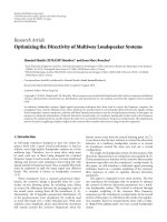
Constrained Real-World Vehicle Trajectory. Normal driving
rules impose a particular trajectory on the vehicle. Indeed,
the curvature of the road and the different lanes constrain
the position of the vehicle. Figure 1 illustrates the pattern of
vehicle trajectories resulting from projective constraints that
can be exploited in vehicle tracking.
Projection of Vehicle Trajectory on the Camera Plane. The
trajectory of a vehicle on the camera plane undergoes severe
distortion due to the low elevation of the traffic surveillance
camera. The curve described by the position of the vehicle
converges asymptotically to the vanishing point.
We propose here to integrate these characteristics to
obtain a finer estimate of the vehicle feature vector. More
specifically, the mapping of real-world vehicle trajectory
through a fractional transform enables a better estimate of
the posterior density. A particle filter is thus implemented,
which integrate cues of the projection in the importance
density, resulting in a better exploration of the state space
and a reduction of the variance in the trajectory estimation.
Preliminary results of this work have been presented in [34];
this paper develops the work further. Its main contribu-
tions are: (i) a complete description of the homographic
projection problem for vehicle tracking and a review of

the solutions proposed to date; (ii) an evaluation of the
projective particle filter tracking rate on a comprehensive
dataset comprising around 2,600 vehicles; (iii) an evaluation
of the resampling accuracy for the projective particle filter;
(iv) a comparison of the performance of the projective
particle filter and the standard particle filter using three
different measures, namely, the sampling frequency, the
mean squared error and tracking drift. The rest of the
paper is organized as follows. Section 2 introduces the
general particle filtering framework. Section 3 develops
theproposedProjectiveParticleFilter(PPF).Ananaly-
sis of the PPF performance versus the standard parti-
cle filter is presented in Section 4 before concluding in
Section 5.
EURASIP Journal on Image and Video Processing 3
(a)
0
20
40
60
80
100
120
140
Position on the image (x)
0 50 100 150 200 250 300 350 400 450 500
Ground distance from the camera (r)
(b)
Figure 1: Examples of vehicle trajectories from a traffic monitoring video sequence. Most vehicles follow a predetermined path: (a) vehicle
trajectories in the image; (b) vehicle positions in the image w.r.t. the distance from the monitoring camera.

2. Bayesian and Part icle Filtering
This section presents a brief review of Bayesian and particle
filtering. Bayesian filtering provides a convenient framework
for object tracking due to the weak assumptions on the
state space model and the first-order Markov chain recursive
properties. Without loss of generality, let us consider a system
with state x of dimension n and observation z of dimension
m.Letx
1:k
{x
1
, , x
k
} and z
1:k
{z
1
, , z
k
} denote,
respectively, the set of states and the set of observations prior
to and including time instant t
k
. The state space model can
be expressed as
x
k
= f
(
x

k−1
)
+ v
k−1
,(1)
z
k
= h
(
x
k
)
+ n
k
,(2)
when the process and observation noises, v
k−1
and n
k
,
respectively, are assumed to be additive. The vector-valued
functions f and h are the process and observation functions,
respectively. Bayesian filtering aims to estimate the posterior
probability density function (pdf) of the state x given the
observation z as p(x
k
| z
k
). The probability density function
is estimated recursively, in two steps: prediction and update.

First, let us denote by p(x
k−1
| z
k−1
)theposterior pdf at time
t
k−1
, and let us assume it is known. The prediction stage relies
on the Chapman-Kolmogorov equation to estimate the prior
pdf p(x
k
| z
k−1
):
p
(
x
k
| z
k−1
)
=

p
(
x
k
| x
k−1
)

p
(
x
k−1
| z
k−1
)
dx
k−1
. (3)
When a new observation becomes available, the prior is
updated as follows:
p
(
x
k
| z
k
)
= λ
k
p
(
z
k
| x
k
)
p
(

x
k
| z
k−1
)
,(4)
where p(z
k
| x
k
) is the likelihood function and λ
k
is a
normalizing constant, λ
k
=

p(z
k
| x
k
)p(x
k
| z
k−1
)dx
k
.
As the posterior probability density function p(x
k

| z
k
)is
recursively estimated through (3)and(4), only the initial
density p(x
0
| z
0
)istobeknown.
Monte Carlo methods and more specifically particle
filters have been extensively employed to tackle the Bayesian
problem represented by (3)and(4)[36, 37]. Multimodality
enables the system to evolve in time with several hypotheses
on the state in parallel. This property is practical to corrobo-
rate or reject an eventual track after several frames. However,
the Bayesian problem then cannot be solved in closed form,
as in the Kalman filter, due to the complex density shapes
involved. Particle filters rely on Sequential Monte Carlo
(SMC) simulations, as a numerical method, to circumvent
the direct evaluation of the Chapman-Kolmogorov equation
(3). Let us assume that a large number of samples
{x
i
k
, i =
1 ···N
S
} are drawn from the posterior distribution p(x
k
|

z
k
). It follows from the law of large numbers that
p
(
x
k
| z
k
)
≈
N
S

i=1
w
i
k
δ

x
k
− x
i
k

,(5)
where w
i
k

are positive weights, satisfying

w
i
k
= 1, and
δ(
·) is the Kronecker delta function. However, because it
is often difficult to draw samples from the posterior pdf,
an importance density q(
·) is used to generate the samples
x
i
k
. It can then be shown that the recursive estimate of the
posterior density via (3)and(4) can be carried out by the set
of particles, provided that the weights are updated as follows
[13]:
w
i
k
∝ w
i
k−1
p

z
k
| x
i

k

p

x
i
k
| x
i
k−1

q

x
i
k
| x
i
k−1
, z
k

=
w
i
k−1
γ
k
p


z
k
| x
i
k

.
(6)
The choice of the importance density q(x
i
k
| x
i
k−1
, z
k
)is
crucial in order to obtain a good estimate of the posterior
pdf. It has been shown that the set of particles and associated
weights
{x
i
k
, w
i
k
} will eventually degenerate, that is, most of
the weights will be carried by a small number of samples
4 EURASIP Journal on Image and Video Processing
H

θ/2
D
x
o
r
αβ
d
X
vp
d
p

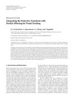
Figure 2: Projection of the vehicle on a plane parallel to the image
plane of the camera. The graph shows a cross-section of the scene
along the direction d (tangential to the road).
and a large number of samples will have negligible weight
[38]. In such a case, and because samples are not drawn
from the true posterior, the degeneracy problem cannot be
avoided and resampling of the set needs to be performed.
Nevertheless, the closer the importance density is from
the true posterior density, the slower the set
{x
i
k
, w
i
k
} will
degenerate; a good choice of importance density reduces the
need for resampling. In this paper, we propose to model the

fractional transform mapping the real world space onto the
cameraplaneandtointegratetheprojectionintheparticle
filter through the importance density q(x
i
k
| x
i
k−1
, z
k
).
3. Projective Particle Filter
TheparticlefilterdevelopedisnamedProjectiveParticle
Filter (PPF) because the vehicle position is projected on the
camera plane and used as an inference to diffuse the particles
in the feature space. One of the particularities of the PPF
is to differentiate between the importance density and the
transition prior pdf, whilst the SIR (Sampling Importance
Resampling) filter, also called standard particle filter, does
not. Therefore, we need to define the importance density
from the fractional transform as well as the transition prior
p(x
k
| x
k−1
) and the likelihood p(z
k
| x
k
) in order to update

the weights in (6).
3.1. Linear Fractional Transformation. The fractional trans-
form is used to estimate the position of the object on the
camera plane (x) from its position on the road (r). The
physical trajectory is projected onto the camera plane as
shown in Figure 2. The distortion of the object trajectory
happens along the direction d, tangential to the road. The
axis d
p
is parallel to the camera plane; the projection x of the
vehicle position on d
p
is thus proportional to the position of
the vehicle on the camera plane. The value of
x is scaled by
X
vp
, the projection of the vanishing point on d
p
,toobtain
the position of the vehicle in terms of pixels. For practical
implementation,itisusefultoexpresstheprojectionalong
the tangential direction d onto the d
p
axis in terms of video
footage parameters that are easily accessible, namely:
(i) angle of view (θ),
(ii) height of the camera (H),
(iii) ground distance (D) between the camera and the first
location captured by the camera.

It can be inferred from Figure 2, after applying the law of
cosines, that
x
2
= r
2
+ 
2
− 2r cos
(
α
)
,(7)

2
=

x
2
+ r
2
− 2rx cos

β

,(8)
where cosα
= (D + r)/

H

2
+(D + r)
2
and β =
arctan(D/H)+θ/2. After squaring and substituting 
2
in (7),
we obtain
r
2


x
2
+ r
2
− 2rx cos β

cos
2
α =

r
2
− rx cos β

2
. (9)
Grouping the terms in
x to get a quadratic form leads to

x
2

cos
2
α − cos
2
β

+2xr

1 − cos
2
α

cos β
+ r
2

cos
2
α − 1

=
0.
(10)
After discarding the nonphysically acceptable solution, one
gets
x
(

r
)
=
rH
(
D + r
)
sin β + H cos β
. (11)
However, because D
 H and θ is small in practice (see
Ta b l e 1), the angle β is approximately equal to π/2and,
consequently, (11) simplifies to
x = rH/(D + r). Note that
this result can be verified using the triangle proportionality
theorem. Finally, we scale
x with the position of the vanishing
point X
vp
in the image to find the position of the vehicle in
terms of pixel location, which yields
x
=
X
vp
lim
r →∞
x
(
r

)
x
(
r
)
=
X
vp
H
x
(
r
)
. (12)
(The position of the vanishing point can either be approx-
imated manually or estimated automatically [39]. In our
experiments, the position of the vanishing point is estimated
manually). The projected speed and the observed size of the
object on the camera plane are also important variables for
the problem of tracking, and hence it is necessary to derive
them. Let v
= dr/dt and
˙
x = dx/dt.Differentiating (12),
after substituting for
x (x = rH/(D + r)) and eliminating r,
yields the observed speed of the vehicle on the camera plane:
˙
x
= f

˙
x
(
x
)
=

X
vp
− x

2
v
X
vp
D
, (13)
Theobservedsizeofthevehicleb can also be derived from
the position x if the real size of the vehicle s is known. If the
center of the vehicle is x, its extremities are located at x + s/2
and x
−s/2. Therefore, applying the fractional transformation
yields
b
= f
b
(
x
)
=

sDX
vp

DX
vp
/(X
vp
− x)

2
−
(
s/2
)
2
. (14)
EURASIP Journal on Image and Video Processing 5
Table 1: Video sequences used for the evaluation of the algorithm performance along with the duration, the number of vehicles, and the
setting parameters, namely, the height (H), the angle of view (θ) and the distance to field of view (D).
Video sequence Duration No. of vehicles Camera height (H)Angleofview(θ)DistancetoFOV(D)
Video 001 199 s 74 6 m 8.5 ± 0.10 deg 48 m
Video
002 360 s 115 5.5 m 15.7 ± 0.12 deg 75 m
Video
003 480 s 252 5.5 m 15.7 ± 0.12 deg 75 m
Video
004 367 s 132 6 m 19.2 ± 0.12 deg 29 m
Video
005 140 s 33 5.5 m 12.5 ± 0.15 deg 80 m
Video

006 312 s 83 5.5 m 19.2 ± 0.2deg 57m
Video
007 302 s 84 5.5 m 19.2 ± 0.2deg 57m
Video
008 310 s 89 5.5 m 19.2 ± 0.2deg 57m
Video
009 80 s 42 5.5 m 19.2 ± 0.2deg 57m
Video
010 495 s 503 7.5 m 6.9 ± 0.15 deg 135 m
Video
011 297 s 286 7.5 m 6.9 ± 0.15 deg 80 m
Video
012 358 s 183 8 m 21.3 ± 0.2deg 43m
Video
013 377 s 188 8 m 21.3 ± 0.2deg 43m
Video
014 278 s 264 6 m 18.5 ± 0.18 deg 64 m
Video
015 269 s 267 6 m 18.5 ± 0.18 deg 64 m
3.2. Importance Density and Transition Prior. The projective
particle filter integrates the fractional transform into the
importance density q(x
i
k
| x
i
k
−1
, z
k

). The state vector x is
modeled with the position, the speed and the size of the
vehicle in the image:
x
=
⎛
⎜
⎜
⎜
⎜
⎜
⎜
⎜
⎜
⎜
⎝
x
y
˙
x
˙
y
b
⎞
⎟
⎟
⎟
⎟
⎟
⎟

⎟
⎟
⎟
⎠
, (15)
where x and y are the Cartesian coordinates of the vehicle,
˙
x and
˙
y are the respective speeds and b is the apparent size
of the vehicle; more precisely, b is the radius of the circle
best fitting the vehicle shape. Object tracking is traditionally
performed using a standard kinematic model (Newton’s
Laws), taking into account the position, the speed and
the size of the object (The size of the object is essentially
maintained for the purpose of likelihood estimation). In this
paper, the kinematic model is refined with the estimation
of the speed and the object size through the fractional
transform along the distorted direction d. Therefore, the
process function f,definedin(1), is given by
f
(
x
k−1
)
=
⎡
⎢
⎢
⎢

⎢
⎢
⎢
⎢
⎢
⎢
⎣
x
k−1
+ f
˙
x
(
x
k−1
)
y
k−1
+
˙
y
k−1
f
˙
x
(
x
k−1
)
˙

y
k−1
f
b
(
x
k−1
)
⎤
⎥
⎥
⎥
⎥
⎥
⎥
⎥
⎥
⎥
⎦
. (16)
It is important to note that since the fractional transform
is along the x-axis, the function f
˙
x
provides a better estimate
than a simple kinematic model taking into account the
speed of the vehicle. On the other hand, the distortion
along the y-axisismuchweakerandsuchanestimation
is not necessary. One novel aspect of this paper is the
estimation of the vehicle position along the x axis and its

size through f
˙
x
and f
b
(x), respectively. It is worthwhile
noting that the standard kinematic model of the vehicle is
recovered when f
˙
x
(x
k−1
) =
˙
x
k−1
and f
b
(x) = b
k−1
.The
vector-valued function g(x
k−1
) ={f(x
k−1
) | f
˙
x
(x
k−1

) =
˙
x
k−1
, f
b
(x) = b
k−1
} denotes the standard kinematic model
in the sequel. The samples of the PPF are drawn from the
importance density q(x
k
| x
k−1
, z
k
) = N (x
k
, f(x
k−1
), Σ
q
)and
the standard kinematic model is used in the prior density
p(x
k
| x
k−1
) = N (x
k

, g(x
k−1
), Σ
p
), where N (·, µ,Σ) denotes
the normal distribution of covariance matrix Σ centered on
µ. The distributions are considered Gaussian and isotropic to
evenly spread the samples around the estimated state vector
at time step k.
3.3. Likelihood Estimation. The estimation of the likelihood
p(z
k
| x
i
k
) is based on the distance between color his-
tograms, as in [40]. Let us define an M-bin histogram
H
= {H[u]}
u=1···M
, representing the distribution of J color
pixel values c, as follows:
H
[
u
]
=
1
J
J


i=1
δ

κ

c
i

−
u

, (17)
where u is the set of bins regularly spaced on the interval
[1, M], κ is a linear binning function providing the bin index
of pixel value c
i
,andδ(·) is the Kronecker delta function.
The pixels c
i
are selected from a circle of radius b centered
on (x, y). Indeed, after projection on the camera plane, the
circle is the standard shape that delineates the vehicle best.
Let us denote the target and the candidate histograms by
6 EURASIP Journal on Image and Video Processing
H
t
and H
x
, respectively. The Bhattacharyya distance between

two histograms is defined as
Δ
(
x
)
=
⎛
⎝
1 −
M

u=1

H
t
[
u
]
H
x
[
u
]
⎞
⎠
. (18)
Finally, the likelihood p(z
k
| x
i

k
)iscalculatedas
p

z
k
| x
i
k

∝
exp

−
Δ

x
i
k

. (19)
3.4. Projective Particle Filter Implementation. Because most
approaches to tracking take the prior density as importance
density, the samples x
i
k
are directly drawn from the standard
kinematic model. In this paper, we differentiate between
the prior and the importance density to obtain a better
distribution of the samples. The initial state x

0
is chosen
as x
0
= [x
0
, y
0
, 10,0,20]
T
where x
0
and y
0
are the initial
coordinates of the object. The parameters are selected to
cater for the majority of vehicles. The position of the vehicles
(x
0
, y
0
) is estimated either manually or with an automatic
procedure (see Section 4.2). The speed along the x-axis
corresponds to the average pixel displacement for a speed
of 90 km
·h
−1
and the apparent size b is set so that the
elliptical region for histogram tracking encompasses at least
the vehicle. The size is overestimated to fit all cars and most

standard trucks at initialization: the size is then adjusted
through tracking by the particle filters. The value x
0
is used
to draw the set of samples x
i
0
: q(x
0
| z
0
) = N (x
i
0
, f(x
0
), Σ
q
).
The transition prior p(x
k
| x
k−1
) and the importance
density q(x
k
| x
k−1
, z
k

) are both modeled with normal
distributions. The prior covariance matrix and mean are
initialized as Σ
p
= diag([6 1 1 1 4]) and µ
p
= g(x
0
),
respectively, and Σ
q
= diag([1 1 0.514])andµ
q
= f(x
0
),
for the importance density. These initializations represent the
physical constraints on the vehicle speed.
A resampling scheme is necessary to avoid the degeneracy
of the particle set. Systematic sampling [41] is performed
when the variance of the weight set is too large, that is, when
the number of the effective samples N
eff
falls below a given
threshold N, arbitrarily set to 0.6N
S
in the implementation.
The number of effective samples N
eff
is evaluated as

N
eff
=
1

N
S
i=1

w
i
k

2
. (20)
The implementation of the projective particle filter algorithm
is summarized in Algorithm 1.
4. Experiments and Results
In this section, the performances of the standard and the
projective particle filters are evaluated on traffic surveillance
data. Since the two vehicle tracking algorithms possess
the same architecture, the difference in performance can
be attributed to the distribution of particles through the
importance density integrating the projective transform. The
experimental results presented in this section aim to evaluate
Require: x
i
0
∼ q(x
0

| z
0
)andw
i
0
= 1/N
S
for i = 1toN
S
do
Compute f(x
i
k
−1
)from(16)
Draw x
i
k
∼ q(x
i
k
| x
i
k
−1
, z
k
) = N (x
i
k

, f(x
i
k
−1
), Σ
q
)
Compute the ratio γ
k
= p(x
i
k
| x
i
k
−1
)/q(x
i
k
| x
i
k
−1
, z
k
)
Update weights w
i
k
= w

i
k
−1
× γ
k
p(z
k
| x
k
)
end for
Normalize w
i
k
ifN
eff
<N then
l
= 0
for i
= 1toN
S
do
σ
i
= cumsum(w
i
k
)
while

l
N
S
<σ
i
do
x
l
k
= x
i
k
w
l
k
= 1/N
S
l = l +1
end while
end for
end if
Algorithm 1: Projective particle filter algorithm.
(1) the improvement in sample distribution with the
implementation of the projective transform,
(2) the improvement in the position error of the vehicle
bytheprojectiveparticlefilter,
(3) the robustness of vehicle tracking (in terms of an
increase in tracking rate) due to the fine distribution
of the particles in the feature space.
The algorithm is tested on 15 traffic monitoring video

sequences, labeled Video
001 to Video 015 in Algorithm 1.
The number of vehicles, and the duration of the video
sequences as well as the parameters of the projective
transform are summarized in Table 1. Around 2,600 moving
vehicles are recorded in the set of video sequences. The videos
range from clear weather to cloudy with weak illumination
conditions. The camera was positioned above highways at
a height ranging from 5.5 m to 8 m. Although the camera
was placed at the center of the highways, a shift in the
position has no effect on the performance, be it only for
the earlier detection of vehicles and the length of the vehicle
path. On the other hand, the rotation of the camera would
affect the value of D and the position of the vanishing
point X
vp
. The video sequences are low-definition (128 ×
160) to comply with the characteristics of traffic monitoring
sequences. The video sequences are footage of vehicles
traveling on a highway. Although the roads are straight in
the dataset, the algorithm can be applied to curved roads
with approximation of the parameters over short distances
because the projection tends to linearize the curves in the
image plane.
4.1. Distribution of Samples. An evaluation of the impor-
tance density can be performed by comparing the distribu-
tion of the samples in the feature space for the standard
and the projective particle filters. Since the degeneracy of
EURASIP Journal on Image and Video Processing 7
the particle set indicates the degree of fitting of the

importance density through the number of effective sam-
ples N
eff
(see (20)), the frequency of particle resampling
is an indicator of the similarity between the posterior
and the importance density. Ideally, the importance density
should be the posterior. This is not possible in practice
because the posterior is unknown; if the posterior were
known, tracking would not be required.
First, the mean squared error (MSE) between the true
state of the feature vector and the set of particles is presented
without resampling in order to compare the tracking accu-
racy of the projective and standard particle filters based solely
on the performance of the importance and prior densities,
respectively. Consequently, the fit of the importance density
to the vehicle tracking problem is evaluated. Furthermore,
computing the MSE provides a quantitative estimate of
the error. Since there is no resampling, a large number of
particlesisrequiredinthisexperiment:wechoseN
S
=
300. Figure 3 shows the position MSE for the standard
and the projective particle filters for 80 trajectories in
Video
008 sequence; the average MSEs are 1.10 and 0.58,
respectively.
Second, the resampling frequencies for the projective
and the standard particle filters are evaluated on the entire
dataset. A decrease in the resampling frequency is the result
of a better (i.e., closer to the posterior density) modeling

of the density from which the samples are drawn. The
resampling frequencies are expressed as the percentage of
resampling compared to the direct sampling at each time
step k.Figure4 displays the resampling frequencies across
the entire dataset for each particle filter. On average, the
projective particle filter resamples 14.9% of the time and the
standard particle filter 19.4%, that is, an increase of 30%
between the former and the latter.
For the problem of vehicle tracking, the importance
density q used in the projective particle filter is therefore
more suitable for drawing samples, compared to the prior
density used in the standard particle filter. An accurate
importance density is beneficial not only from a compu-
tational perspective since the resampling procedure is less
frequently called, but also for tracking performance, as the
particles provide a better fit to the true posterior density.
Subsequently,thetrackerislesspronetodistractionincase
of occlusion or similarity between vehicles.
4.2. Trajectory Error Evaluation. An important measure in
vehicle tracking is the variance of the trajectory. Indeed,
high-level tasks, such as abnormal behavior or DUI (driving
under the influence) detection, require an accurate tracking
of the vehicle and, in particular, a low MSE for the position.
Figure 5 displays a track estimated with the projective particle
filter and the standard particle filter. It can be inferred
qualitatively that the PPF achieves better results than the
standard particle filter. Two experiments are conducted to
evaluate the performance in terms of position variance: one
with semiautomatic variance estimation and the other one
with ground truth labeling to evaluate the influence of the

number of particles.
0
0.5
1
1.5
2
2.5
3
3.5
Mean squared error
0 1020304050607080
Track index
Mean squared error for 300 samples without resampling
Projective particle filter
Standard particle filter
Figure 3: Position mean squared error for the standard (solid) and
the projective (dashed) particle filter without resampling step.
0
5
10
15
20
25
30
35
40
45
(%)
M2U00010
M2U00012

M2U00012b
M2U00015
M2U00145
M2U00149
M2U00150
M2U00151
M2U00152
M2U00158
M2U00159
M2U00160
M2U00161
M2U00186
M2U00187
Percentage of resampling
Standard particle filter
Projective particle filter
Figure 4: Resampling frequency for the 15 videos of the dataset.
The resampling frequency is the ratio between the number of
resampling and the number of particle filter iteration. The average
resampling frequency for the projective particle filter is 14.9%, and
19.4% for the standard particle filter.
In the first experiment, the performance of each tracker
is evaluated in terms of MSE. In order to avoid the tedious
task of manually extracting the groundtruth of every track,
a synthetic track is generated automatically based on the
parameters of the real world projection of the vehicle
trajectory on the camera plane. Figure 6 shows that the
theoretic and the manually extracted tracks match almost
perfectly. The initialization of the tracks is performed as in
[35]. However, because the initial position of the vehicle

when tracking starts may differ from one track to another,
it is necessary to align the theoretic and the extracted tracks
in order to cancel the bias in the estimation of the MSE.
Furthermore, the variance estimation is semiautomatic since
the match between the generated and the extracted tracks is
visually assessed. It was found that Video
005, Video 006,
and Video
008 sequences provide the best matches over-
all. The 205 vehicle tracks contained in the 3 sequences
8 EURASIP Journal on Image and Video Processing
120
100
80
60
40
20
20 40 60 80 100 120 140 160
(a) Standard
120
100
80
60
40
20
20 40 60 80 100 120 140 160
(b) Projective
Figure 5: Vehicle track for (a) the standard and (b) the projective particle filter. The projective particle filter exhibits a lower variance in the
position estimation.
20

40
60
80
100
120
Pixel value along the d-axis
0 50 100 150 200 250
Time
Theoretic and ground truth track after alignment
Theoretic track
Ground truth track
Figure 6: Alignment of theoretic and extracted trajectories along
the d-axis. The difference between the two tracks represents error in
the estimation of the trajectory.
Table 2: MSE for the standard and the projective particle filters with
100 samples.
Video sequence Video 005 Video 006 Video 008
Avg. MSE Std PF 2.26 0.99 1.07
Avg. MSE Proj. PF 1.89 0.83 1.02
are matched against their respective generated tracks and
visually inspected to ensure adequate correspondence. The
average MSEs for each video sequence are presented in
Ta b l e 2 for a sample set size of 100. It can be inferred from
Ta b l e 2 that the PPF consistently outperforms the standard
particle filter. It is also worth noting that the higher MSE in
this experiment, compared to the one presented in Figure 5
for Video
008, is due to the smaller number of particles—
even with resampling, the particle filters do not reach the
accuracy achieved with 300 particles.

1
2
3
4
5
6
Mean squared error
0 50 100 150 200 250 300
Number of particles (N
S
)
Position MSE for standard and projective particle filters
Projective particle filter
Standard particle filter
Figure 7: Position mean squared error versus number of particles
for the standard and the projective particle filter.
In the second experiment, we evaluate the performance
of the two tracking algorithms w.r.t. the number of par-
ticles. Here, the ground truth is manually labeled in the
video sequence. This experiment serves as validation to
the semiautomatic procedure described above as well as an
evaluation of the effect of particle set size on the performance
of both the PPF and the standard particle filter. To ensure
the impartiality of the evaluation, we arbitrarily decided
to extract the ground truth for the first 5 trajectories in
Video
001 sequence. Figure 7 displays the average MSE over
10 epochs for the first trajectory and for different values of
N
S

.Figure8 presents the average MSE for 10 epochs on
the 5 ground truth tracks for N
S
= 20 and N
S
= 100.
The experiments are run with several epochs to increase
the confidence in the results due to the stochastic nature
of particle filters. It is clear that the projective particle filter
outperforms the standard particle filter in terms of MSE.
The higher accuracy of the PPF, with all parameters being
EURASIP Journal on Image and Video Processing 9
2
4
6
8
Mean squared error
12345
Track index
Position MSE for 20 particles and 5 different tracks
Projective particle filter
Standard particle filter
(a)
1
2
3
4
Mean squared error
12345
Track index

Position MSE for 100 particles and 5 different tracks
Projective particle filter
Standard particle filter
(b)
Figure 8: Position mean squared error for 5 ground truth labeled vehicles using the standard and the projective particle filter. (a) with 20
particles; (b) with 100 particles.
0
10
20
30
40
50
60
70
80
90
100
Video 001
Video
002
Video
003
Video
004
Video
005
Video
006
Video
007

Video
008
Video
009
Video
0010
Video
0011
Video
0012
Video
0013
Video
0014
Video
0015
Vehicle tracking performance
Standard particle filter
Projective particle filter
Figure 9: Tracking rate for the projective and standard particle
filters on the traffic surveillance dataset.
identical in the comparison, is due to the finer estimation of
the sample distribution by the importance density and the
consequent adjustment of the weights.
4.3. Tracking Rate Evaluation. An important problem
encountered in vehicle tracking is the phenomenon of
tracker drift. We propose here to estimate the robustness of
the tracking by introducing a tracking rate based on drift
measure and to estimate the percentage of vehicles tracked
withoutseveredrift,thatis,forwhichthetrackisnot

lost. The tracking rate primarily aims to detect the loss of
vehicle track and, therefore, evaluates the robustness of the
tracker. Robustness is differentiated from accuracy in that
the former is a qualitative measure of tracking performance
while the latter is a quantitative measure, based on an error
measure as in Section 4.2,forinstance.Thedriftmeasurefor
vehicle tracking is based on the observation that vehicles are
converging to the vanishing point; therefore, the trajectory
of the vehicle along the tangential axis is monotonically
decreasing. As a consequence, we propose to measure the
number of steps where the vehicle position decreases (p
d
)
and the number of steps where the vehicle position increases
or is constant (p
i
), which is characteristic of drift of a
tracker. Note that horizontal drift is seldom observed since
thedistortionalongthisaxisisweak.Therateofvehicles
tracked without severe drift is then calculated as
Tr ac ki ng Ra te
=
p
d
p
d
+ p
i
. (21)
The tracking rate is evaluated for the projective and

standard particle filters. Figure 9 displays the results for the
entire traffic surveillance dataset. It shows that the projective
particle filter yields better tracking rate than the standard
particle filter across the entire dataset. The projective particle
filter improves the tracking rate compared to the standard
particle filter. Figure 9 also shows that the difference between
the tracking rates is not as important as the difference in
MSE because the second one already performs well on vehicle
tracking. At a high-level, the projective particle filter still
yields a reduction in the drift of the tracker.
4.4. Discussion. The experiments show that the projective
particle filter performs better than the standard particle filter
in terms of sample distribution, tracking error and tracking
rate. The improvement is due to the integration of the pro-
jective transform in the importance density. Furthermore,
the implementation of the projective transform requires
very simple calculations under simplifying assumptions (12).
Overall, since the projective particle filter requires fewer
samples than the standard particle filter to achieve better
tracking performance, the increase in computation due
totheprojectivetransformisoffset by the reduction in
sample set size. More specifically, the projective particle
filter requires the computation of the vector-valued process
function and the ratio γ
k
for each sample. For the process
function, (13)and(14), representing f
˙
x
(x)and f

b
(x),
respectively, must be computed. The computation burden is
low assuming that constant terms can be precomputed. On
the other hand, the projective particle filter yields a gain in
the sample set size since less particles are required for a given
error and the resampling is 30% more efficient.
10 EURASIP Journal on Image and Video Processing
The projective particle filter performs better on the
three different measures. The projective transform leads to
a reduction in resampling frequency since the distribution
of the particles carries accurately the posterior and, con-
sequently, the degeneracy of the particle set is slower. The
mean squared error is reduced since the particles focus
around the actual position and size of the vehicle. The
driftratebenefitsfromtheprojectivetransformsincethe
tracker is less distracted by similar objects or by occlusion.
The improvement is beneficial for applications that require
vehicle “locking” such as vehicle counts or other applications
for which performance is not based on the MSE. It is
worthwhile noting here that the MSE and the tracking rate
are independent: it can be observed from Figure 9 that the
tracking rate is almost the same for Video
005, Video 006,
and Video
008, but there is a factor of 2 between the MSE’s
of Video
005 and Video 008 (see Table 2).
5. Conclusion
A plethora of algorithms for object tracking based on

Bayesian filtering are available. However, these systems fail
to take advantage of traffic monitoring characteristics, in
particular slow-varying vehicle speed, constrained real-world
vehicle trajectory and projective transform of vehicles onto
the camera plane. This paper proposed a new particle filter,
namely, the projective particle filter, which integrates these
characteristics into the importance density. The projective
fractional transform, which maps the real world position of a
vehicle onto the camera plane, provides a better distribution
of the samples in the feature space. However, since the prior
is not used for sampling, the weights of the projective particle
filter have to be readjusted. The standard and the projective
particle filters have been evaluated on traffic surveillance
videos using three different measures representing robust
and accurate vehicle tracking: (i) the degeneracy of the
sample set is reduced when the fractional transform is
integrated within the importance density; (ii) the tracking
rate, measured through drift evaluation, shows an improve-
ment in robustness of the tracker; (iii) the MSE on the
vehicle trajectory is reduced with the projective particle
filter. Furthermore, the proposed technique outperforms the
standard particle filter in terms of MSE even with a fewer
number of particles.
References
[1] Y.K.JungandYO.S.Ho,“Traffic parameter extraction using
video-based vehicle tracking,” in Proceedings of IEEE/IEEJ/JSAI
International Conference on Intelligent Transportation Systems,
pp. 764–769, October 1999.
[2] J. M
´

elo, A. Naftel, A. Bernardino, and J. Santos-Victor, “Detec-
tion and classification of highway lanes using vehicle motion
trajectories,” IEEE Transactions on Intelligent Transportation
Systems, vol. 7, no. 2, pp. 188–200, 2006.
[3] C.P.Lin,J.C.Tai,andK.T.Song,“Traffic monitoring based
on real-time image tracking,” in Proceedings of IEEE Interna-
tional Conference on Robotics and Automation, pp. 2091–2096,
September 2003.
[4]Z.Qiu,D.An,D.Yao,D.Zhou,andB.Ran,“Anadaptive
Kalman Predictor applied to tracking vehicles in the traffic
monitoring system,” in Proceedings of IEEE Intelligent Vehicles
Symposium, pp. 230–235, June 2005.
[5] F. Dellaert, D. Pomerleau, and C. Thorpe, “Model-based car
tracking integrated with a road-follower,” in Proceedings of
IEEE International Conference on Robotics and Automation,
vol. 3, pp. 1889–1894, 1998.
[6] J. Y. Choi, K. S. Sung, and Y. K. Yang, “Multiple vehicles
detection and tracking based on scale-invariant feature trans-
form,” in Proceedings of the 10th International IEEE Conference
on Intelligent Transportation Systems (ITSC ’07), pp. 528–533,
October 2007.
[7] D. Koller, J. Weber, and J. Malik, “Towards realtime visual
based tracking in cluttered trafficscenes,”inProceedings of the
Intelligent Vehicles Symposium, pp. 201–206, October 1994.
[8] E. B. Meier and F. Ade, “Tracking cars in range images using
the condensation algorithm,” in Proceedings of IEEE/IEEJ/JSAI
International Conference on Intelligent Transportation Systems,
pp. 129–134, October 1999.
[9] T. Xiong and C. Debrunner, “Stochastic car tracking with line-
and color-based features,” in Proceedings of IEEE Conference on

Intelligent Transportation Systems, vol. 2, pp. 999–1003, 2003.
[10] M. A. Isard, Visual motion analysis by probabilistic propagation
of conditional density, Ph.D. thesis, University of Oxford,
Oxford, UK, 1998.
[11] M. Isard and A. Blake, “Condensation—conditional density
propagation for visual tracking,” International Journal of
Computer Vision, vol. 29, no. 1, pp. 5–28, 1998.
[12] A. Doucet, “On sequential simulation-based methods for
Bayesian filtering,” Tech. Rep., University of Cambridge,
Cambridge, UK, 1998.
[13] M. S. Arulampalam, S. Maskell, N. Gordon, and T. Clapp, “A
tutorial on particle filters for online nonlinear/non-Gaussian
Bayesian tracking,” IEEE Transactions on Signal Processing,
vol. 50, no. 2, pp. 174–188, 2002.
[14] R. Van Der Merwe, A. Doucet, N. De Freitas, and E. Wan, “The
unscented particle filter,” Tech. Rep., Cambridge University
Engineering Department, 2000.
[15] J. H. Kotecha and P. M. Djuri
´
c, “Gaussian sum particle
filtering,” IEEE Transactions on Signal Processing, vol. 51,
no. 10, pp. 2602–2612, 2003.
[16] C. Chang and R. Ansari, “Kernel particle filter for visual
tracking,” IEEE Signal Processing Letters, vol. 12, no. 3, pp. 242–
245, 2005.
[17] C. Chang, R. Ansari, and A. Khokhar, “Multiple object
tracking with kernel particle filter,” in Proceedings of IEEE
Computer Society Conference on Computer Vision and Pattern
Recognition (CVPR ’05), pp. 568–573, June 2005.
[18] L. Liang-qun, J. Hong-bing, and L. Jun-hui, “The iterated

extended kalman particle filter,” in Proceedings of the Inter-
national Symposium on Communications and Information
Technologies (ISCIT ’05), pp. 1213–1216, 2005.
[19]C.Kwok,D.Fox,andM.Meil
ˇ
a, “Adaptive real-time particle
filters for robot localization,” in Proceedings of IEEE Interna-
tional Conference on Robotics and Automation, pp. 2836–2841,
September 2003.
[20] C. Kwok, D. Fox, and M. Meil
ˇ
a, “Real-time particle filters,”
Proceedings of the IEEE, vol. 92, no. 3, pp. 469–484, 2004.
[21]C.Shen,M.J.Brooks,andA.D.vanHengel,“Augmented
particle filtering for efficient visual tracking,” in Proceedings of
IEEE International Conference on Image Processing (ICIP ’05),
pp. 856–859, September 2005.
EURASIP Journal on Image and Video Processing 11
[22] Z. Zeng and S. Ma, “Head tracking by active particle filtering,”
in Proceedings of IEEE Conference on Automatic Face and
Gesture Recognition, pp. 82–87, 2002.
[23] R. Feghali and A. Mitiche, “Spatiotemporal motion boundary
detection and motion boundary velocity estimation for track-
ing moving objects with a moving camera: a level sets PDEs
approach with concurrent camera motion compensation,”
IEEE Transactions on Image Processing, vol. 13, no. 11, pp.
1473–1490, 2004.
[24] C. Yang, R. Duraiswami, and L. Davis, “Fast multiple object
tracking via a hierarchical particle filter,” in Proceedings of
the 10th IEEE International Conference on Computer Vision

(ICCV ’05), pp. 212–219, October 2005.
[25] J. Li and C S. Chua, “Transductive inference for color-based
particle filter tracking,” in Proceedings of IEEE International
Conference on Image Processing, vol. 3, pp. 949–952, September
2003.
[26] P. Vadakkepat and L. Jing, “Improved particle filter in
sensor fusion for tracking randomly moving object,” IEEE
Transactions on Instrumentation and Measurement, vol. 55,
no. 5, pp. 1823–1832, 2006.
[27] A. Ziadi and G. Salut, “Non-overlapping deterministic Gaus-
sian particles in maximum likelihood non-linear filtering.
Phase tracking application,” in Proceedings of the International
Symposium on Intelligent Sign al Processing and Communication
Systems (ISPACS ’05), pp. 645–648, December 2005.
[28] J. Czyz, “Object detection in video via particle filters,” in
Proceedings of the 18th International Conference on Pattern
Recognition (ICPR ’06), pp. 820–823, August 2006.
[29]M.W.WoolrichandT.E.Behrens,“Variationalbayes
inference of spatial mixture models for segmentation,” IEEE
Transactions on Medical Imaging, vol. 25, no. 10, pp. 1380–
1391, 2006.
[30] K. Nickel, T. Gehrig, R. Stiefelhagen, and J. McDonough,
“A joint particle filter for audio-visual speaker tracking,” in
Proceeding of the 7th International Conference on Multimodal
Interfaces (ICMI ’05), pp. 61–68, October 2005.
[31] E. Bas¸, A. M. Tekalp, and F. S. Salman, “Automatic vehicle
counting from video for traffic flow analysis,” in Proceedings
of IEEE Intelligent Vehicles Symposium (IV ’07), pp. 392–397,
June 2007.
[32] B. Gloyer, H. K. Aghajan, K Y. Siu, and T. Kailath, “Vehicle

detection and tracking for freeway traffic monitoring,” in
Proceedings of the Asilomar Conference on S ignals, Systems and
Computers, vol. 2, pp. 970–974, 1994.
[33] L. Zhao and C. Thorpe, “Qualitative and quantitative car
tracking from a range image sequence,” in Proceedings of the
IEEE Computer Society Conference on Computer Vision and
Pattern Recognition, pp. 496–501, June 1998.
[34] P. L. M. Bouttefroy, A. Bouzerdoum, S. L. Phung, and A.
Beghdadi, “Vehicle tracking using projective particle filter,”
in Proceedings of the 6th IEEE International Conference on
Advanced Video and Signal Based Surveillance (AVSS ’09),
pp. 7–12, September 2009.
[35] P. L. M. Bouttefroy, A. Bouzerdoum, S. L. Phung, and
A. Beghdadi, “Vehicle tracking by non-drifting mean-shift
using projective kalman filter,” in Proceedings of the 11th
International IEEE Conference on Intelligent Transportation
Systems (ITSC ’08), pp. 61–66, December 2008.
[36] F. Gustafsson, F. Gunnarsson, N. Bergman et al., “Particle
filters for positioning, navigation, and tracking,” IEEE Trans-
actions on Signal Processing, vol. 50, no. 2, pp. 425–437, 2002.
[37] Y. Rathi, N. Vaswani, and A. Tannenbaum, “A generic
framework for tracking using particle filter with dynamic
shape prior,” IEEE Transactions on Image Processing, vol. 16,
no. 5, pp. 1370–1382, 2007.
[38] A. Kong, J. S. Lui, and W. H. Wong, “Sequential imputations
and bayesian missing data problems,” Journal of the American
Statistical Assocation, vol. 89, no. 425, pp. 278–288, 1994.
[39] D. Schreiber, B. Alefs, and M. Clabian, “Single camera lane
detection and tracking,” in Pr oceedings of the 8th International
IEEE Conference on Intelligent Transportation Syste ms, pp. 302–

307, September 2005.
[40] D. Comaniciu, V. Ramesh, and P. Meer, “Kernel-based object
tracking,” IEEE Transactions on Pattern A nalysis and Machine
Intelligence, vol. 25, no. 5, pp. 564–577, 2003.
[41] G. Kitagawa, “Monte Carlo filter and smoother for non-
Gaussian nonlinear state space models,” Journal of Computa-
tional and Graphical Statistics, vol. 5, no. 1, pp. 1–25, 1996.