Báo cáo hóa học: " Research Article A New Bigram-PLSA Language Model for Speech Recognition" potx

Hindawi Publishing Corporation
EURASIP Journal on Advances in Signal Processing
Volume 2010, Article ID 308437, 8 pages
doi:10.1155/2010/308437
Research Article
A New Bigram-PLSA Language Model for Speech Recognition
Mohammad Bahrani and Hossein Sameti
Department of Computer Engineering, Sharif University of Technology, 145-8889694 Tehran, Iran
Correspondence should be addressed to Mohammad Bahrani,
Received 3 March 2010; Revised 9 May 2010; Accepted 8 July 2010
Academic Editor: Douglas O’Shaughnessy
Copyright © 2010 M. Bahrani and H. Sameti. This is an open access article distributed under the Creative Commons Attribution
License, which permits unrestricted use, distribution, and reproduction in any medium, provided the original work is properly
cited.
A novel method for combining bigram model and Probabilistic Latent Semantic Analysis (PLSA) is introduced for language
modeling. The motivation behind this idea is the relaxation of the “bag of words” assumption fundamentally present in latent
topic models including the PLSA model. An EM-based parameter estimation technique for the proposed model is presented in
this paper. Previous attempts to incorporate word order in the PLSA model are surveyed and compared with our new proposed
model both in theory and by experimental evaluation. Perplexity measure is employed to compare the effectiveness of recently
introduced models with the new proposed model. Furthermore, experiments are designed and carried out on continuous speech
recognition (CSR) tasks using word error rate (WER) as the evaluation criterion. The superiority of the new bigram-PLSA model
over Nie et al.’s bigram-PLSA and simple PLSA models is demonstrated in the results of our experiments. Exper iments on BLLIP
WSJ corpus show about 12% reduction in p erplexity and 2.8% WER improvement compared to Nie et al.’s bigram-PLSA model.
1. Introduction
Language models are important in various applications
especially in speech recognition. Statistical language models
are obtained using different approaches depending on the
resources and tasks requirements. Extracting n-gram statis-
tics is a prevalent approach for statistical language modeling.
N-gram takes the order of words into account and calculates
the probability of the word occurring after n

−1 other known
words.
Many attempts have been made to incorporate semantic
knowledge in language modeling. Latent topic modeling
approaches such as Latent Semantic Analysis (LSA) [1,
2], Probabilistic Latent Semantic Analysis (PLSA) [3], and
Latent Dirichlet Allocation (LDA) [4] are the most recent
techniques. Latent semantic information is extracted by these
models through decomposing word-document cooccurrence
matrix. These topic models have been successful in reducing
the perplexity and improving the accuracy rate of speech
recognition systems [2, 5, 6]. The main deficiency of the
topic models is that they do not take the order of words
into consideration due to the assumption of “bag of words”
intrinsically.
The useful semantic modeling of the topic models
and the potential of considering words history in the n-
gram language model motivate researchers to combine the
capabilities of both approaches. Bellegarda [2] proposed
the combination of the n-gram and the LSA models and
Federico [7] utilized the PLSA framework to adapt the n-
gram language model. Both [2, 7]usedrescalingapproach
for the combination. Griffiths et al. [8]presentedan
extension of the topic model that is sensitive to word order
and automatically learns the syntactic factors as well as
the semantic ones. In [9, 10] the collocation of words
was incorporated in the LDA model. Girolami and Kaban
[11] relaxed the “bag of words” assumption in the LDA
model by applying the Markov chain assumption on symbol
sequences. Wallach [12] proposed a combination of bigram

and LDA models (the bigram topic model) and achieved
a significant performance improvement on perplexity by
exploring latent semantics following different context words.
This research was a basis for Nie et al.’s work [13] that
proposed the combination of bigram and PLSA models. The
performance improvements achieved in [12, 13]motivated
us to propose a general framework for combining bigram
and PLSA models. As discussed in Section 3.6,ourmodel
2 EURASIP Journal on Advances in Signal Processing
is different from Nie et al.’s work and can be considered as
a generalization to that model. One cannot derive the re-
estimation formulae via the standard EM procedure based on
Nie et al.’s model. In this paper, we propose an EM procedure
for re-estimating the parameters of our model.
The remainder of the paper is organized as follows. In
Section 2, the PLSA model is briefly reviewed. In Section 3,
the combination of bigram and PLSA models is introduced
and its parameter estimation procedure is described. In
Section 4, experimental results are presented and finally in
Section 5 the conclusions are made.
2. Review of the PLSA Model
Suppose that we have a set of words W ={w
1
, w
2
, , w
M
}
that composes a set of documents D ={d
1

, d
2
, , d
N
}.In
the PLSA model, the occurrence probability of word w
i
given
document d
j
is defined as below [3].
P

w
i
| d
j

=

k
P
(
w
i
| z
k
)
P


z
k
| d
j

,(1)
where z
k
is a latent class variable (or a topic) belonging
to a set of class variables (topics) Z
={z
1
, z
2
, , z
K
}.
Equation (1) is a weighted mixture of word distributions
called aspect model [14]. The aspect model is a latent variable
model for co-occurrence data that associates an unobserved
class var iable z
k
∈ Z to each observation (i.e., words
and documents). The aspect model introduces a conditional
independence assumption, that is, d
j
and w
i
are independent
conditioned on the state of the associated latent variable [15].

In (1), P(w
i
| z
k
), i = 1, , M, k = 1, , K are the word
distributions and P(z
k
| d
j
), k = 1, , K, j = 1, , N are
the weights of distributions.
In another view, the PLSA model is a decomposition of
word-document co-occurrence matrix P(w
| d). The P(w |
d)matrixisdecomposedintoP(w | z)andP(z | d)matrices
in order to minimize the cross entropy (KL divergence)
between the P(w
| d) matrix and empirical distribution.
The PLSA parameters P(w
i
| z
k
)andP(z
k
| d
j
)are
re-estimated via the EM procedure. The EM procedure
includes two alternate steps: ( i) an expectation (E) step where
posterior probabilities are computed for the latent variables

based on the current estimates of the parameters, (ii) a
maximization (M) step where PLSA parameters are updated
based on the posterior probabilities computed in the E-step
[15].
3. Combining Bigram and PLSA Models
Before describing the proposed model, the previous research
on combining bigram and PLSA model by Nie et al. [13]
is reviewed. This method is a special case (with certain
independence assumptions) of our proposed method.
3.1. Nie et al.’s Bigram-PLSA Model. Nie et al. presented a
combination of bigram and PLSA models [13]. Instead of
P(w
i
| z
k
)in(1), their bigram-PLSA model employs P(w
j
|
w
i
, z
k
) resulting in
P

w
j
| w
i
, d

k

=

l
P

w
j
| w
i
, z
l

P
(
z
l
| d
k
)
. (2)
The EM procedure for training the combined model
contains the following two steps.
E-step:
P

z
l
| d

k
, w
i
, w
j

=
P

w
j
| w
i
, z
l

P
(
z
l
| d
k
)

l

P

w
j

| w
i
, z
l


P
(
z
l

| d
k
)
. (3)
M-step:
P

w
j
| w
i
, z
l

=

k
n


d
k
, w
i
, w
j

P

z
l
| d
k
, w
i
, w
j


j


k
n

d
k
, w
i
, w

j


P

z
l
| d
k
, w
i
, w
j


,
(4)
P
(
z
l
| d
k
)
=

j

i
n


d
k
, w
i
, w
j

P

z
l
| d
k
, w
i
, w
j

N
(
d
k
)
,(5)
where n(d
k
, w
i
, w

j
) is the number of times that the word pair
w
i
w
j
occurs in the document d
k
, and N(d
k
) is the number of
words in the document d
k
.
3.2. Proposed Bigram-PLSA Model. We intend to combine
the bigram and the PLSA models to take advantage of the
strengths of both models for increasing the predictability of
wordsindocuments.InordertocombinebigramandPLSA
models, we incorporate the context word w
i
in the PLSA
parameters. In other words, we associate the generation of
words and documents to the context word in a ddition to the
latent topics.
The generative process of bigram-PLSA model can be
defined by the following scheme:
(1) Generate a context word w
i
as the word history with
probability P(w

i
).
(2) Select a document d
k
with probability P(d
k
| w
i
).
(3) Pick a latent variable z
l
with probability P(z
l
| w
i
, d
k
).
(4) Generate a word w
j
with probability P(w
j
| w
i
, z
l
).
Translating the generative process into a joint probability
model results in
P


d
k
, w
i
, w
j

=
P

d
k
, w
i
w
j

=

l
P
(
w
i
)
P
(
d
k

| w
i
)
P
(
z
l
| w
i
, d
k
)
× P

w
j
| w
i
, z
l

.
(6)
EURASIP Journal on Advances in Signal Processing 3
According to (6), the occurrence probability of the word
w
j
given the document d
k
and the word history w

i
is defined
as
P

w
j
| w
i
, d
k

=

l
P

w
j
| w
i
, z
l

P
(
z
l
| w
i

, d
k
)
. (7)
Equation (7) is an extended version of the aspect model
that considers the word history in the word-document
modeling and can be considered as a combination of bigram
and PLSA models. In (7), the distributions P(w
j
| w
i
, z
l
)
and P(z
l
| w
i
, d
k
) are the model parameters that should be
estimated from training data. This model is similar to the
original PLSA model except that the context words (word
history) w
i
is incorporated in the model parameters.
Like the original aspect model, the extended aspect
model assumes conditional independence between word
w
j

and document d
k
, that is, w
j
and d
k
are independent
conditioned on the latent parameter z
l
and the context word
w
i
:
P

d
k
, w
j
| w
i
, z
l

=
P
(
d
k
| w

i
, z
l
)
P

w
j
| w
i
, z
l

. (8)
The justification behind the assumed conditional inde-
pendence in the proposed model is the same reasoning that
the PLSA model is using to make an analytical model, that
is, simplification of the model formulation and reasonable
reduction of the computational cost.
As in the original PLSA model, the equivalent parameter-
ization of the joint probability in (6)canbewrittenas
P

d
k
, w
i
, w
j


=
P
(
w
i
)

l
P

w
j
| w
i
, z
l

P
(
d
k
| w
i
, z
l
)
P
(
z
l

| w
i
)
.
(9)
3.3. Parameter Estimation Using the EM Algorithm. Like
original PLSA model, we re-estimate the parameters of
bigram-PLSA model using the EM procedure. In the EM
procedure, for E-step, we simply apply Bayes’ rule to obtain
the posterior probability of the latent var iable z
l
given the
observed data d
k
, w
i
,andw
j
.
E-step:
P

z
l
| d
k
, w
i
, w
j


=
P

z
l
, d
k
, w
i
, w
j


l

P

z
l

, d
k
, w
i
, w
j

=
P

(
w
i
, z
l
)
P
(
d
k
| w
i
, z
l
)
P

w
j
| w
i
, z
l


l

P
(
w

i
, z
l

)
P
(
d
k
| w
i
, z
l

)
P

w
j
| w
i
, z
l


.
(10)
We can rewr ite (10)as
P


z
l
| d
k
, w
i
, w
j

=
P
(
z
l
| w
i
)
P
(
d
k
| w
i
, z
l
)
P

w
j

| w
i
, z
l


l

P
(
z
l

| w
i
)
P
(
d
k
| w
i
, z
l

)
P

w
j

| w
i
, z
l


=
P

w
j
| w
i
, z
l

P
(
z
l
| w
i
, d
k
)

l

P


w
j
| w
i
, z
l


P
(
z
l

| w
i
, d
k
)
.
(11)
In the M-step, the parameters are updated by max-
imizing the log-likelihood of the complete data (words
and documents) with respect to the probabilistic model.
The likelihood of the complete data with respect to the
probabilistic model is computed as
L
=

i, j,k
P(d

k
, w
i
w
j
)
n(d
k
,w
i
w
j
)
, (12)
where P(d
k
, w
i
w
j
) is the occurrence probability of the word
pair w
i
w
j
in the document d
k
and n(d
k
, w

i
w
j
) is the
frequency of word pair w
i
w
j
in the document d
k
.
Let θ
={P(w
j
| w
i
, z
l
), P(z
l
| w
i
, d
k
)} be the set
of model parameters. For estimating θ, we use MLE to
maximize the log-likelihood of the complete data:
θ
ML
= arg max

θ
log
(
L
)
= arg max
θ

i, j,k
n

d
k
, w
i
w
j

log P

d
k
, w
i
w
j

=
arg max
θ


i, j,k
n

d
k
, w
i
w
j

×

log P
(
d
k
, w
i
)
+logP

w
j
| w
i
, d
k

.

(13)
Considering (7), we expand the above equation to
θ
ML
= arg max
θ

i, j,k
n

d
k
, w
i
w
j

log P
(
d
k
, w
i
)
+

i, j,k
n

d

k
, w
i
w
j

log
⎛
⎝

l
P

w
j
| w
i
, z
l

P
(
z
l
| w
i
, d
k
)
⎞

⎠
=
arg max
θ

i, j,k
n

d
k
, w
i
w
j

×
log
⎛
⎝

l
P

w
j
| w
i
, z
l


P
(
z
l
| w
i
, d
k
)
⎞
⎠
.
(14)
In (14), the left factor before the plus sign is omitted
because it is independent of θ. In order to maximize the log-
likelihood, (14) should be differentiated. Differentiating (14)
with respect to the parameters does not lead to well-formed
4 EURASIP Journal on Advances in Signal Processing
formulae, so we try to find a lower bound for (14) using
Jensen’s inequality

i, j,k
n

d
k
, w
i
w
j


log
⎛
⎝

l
P

w
j
| w
i
, z
l

P
(
z
l
| w
i
, d
k
)
⎞
⎠
=

i, j,k
n


d
k
, w
i
w
j

×
log
⎛
⎝

l
P

z
l
| d
k
, w
i
, w
j

P

w
j
| w

i
, z
l

P
(
z
l
| w
i
, d
k
)
P

z
l
| d
k
, w
i
, w
j

⎞
⎠
≥

i, j,k
n


d
k
, w
i
w
j


l
P

z
l
| d
k
, w
i
, w
j

×
log
⎛
⎝
P

w
j
| w

i
, z
l

P
(
z
l
| w
i
, d
k
)
P

z
l
| d
k
, w
i
, w
j

⎞
⎠
.
(15)
The obtained lower bound should be maximized, that is,
maximizing the right hand side of (15) instead of its left hand

side. For maximizing the lower bound and re-estimating
the parameters, we have a constrained optimization problem
because all parameters indicate probability distributions.
Therefore, the parameters should satisfy the constraints

j
P

w
j
| w
i
, z
l

=
1 ∀i, l,

l
P
(
z
l
| w
i
, d
k
)
= 1 ∀i, k.
(16)

In order to consider the above constraints, the right hand
side of (15) has to be augmented by the appropriate Lagrange
multipliers
H
=

i, j,k
n

d
k
, w
i
w
j


l
P

z
l
| d
k
, w
i
, w
j

×

log
⎛
⎝
P

w
j
| w
i
, z
l

P
(
z
l
| w
i
, d
k
)
P

z
l
| d
k
, w
i
, w

j

⎞
⎠
+

i,l
τ
il
⎛
⎝
1 −

j
P

w
j
| w
i
, z
l

⎞
⎠
+

i,k
ρ
ik

⎛
⎝
1 −

l
P
(
z
l
| w
i
, d
k
)
⎞
⎠
,
(17)
where τ
il
and ρ
ik
are the Lagrange multipliers related to
constraints specified in (16).
Differentiating the above equation partially with respect
to the different parameters leads to(18)
∂H
∂P

w

j
| w
i
, z
l

=

k
n

d
k
, w
i
w
j

P

z
l
| d
k
, w
i
, w
j

P


w
j
| w
i
, z
l

−
τ
il
= 0,
∂H
∂P
(
z
l
| w
i
, d
k
)
=

j
n

d
k
, w

i
w
j

P

z
l
| d
k
, w
i
, w
j

P
(
z
l
| w
i
, d
k
)
− ρ
il
= 0.
(18)
Solving (18) and applying the constraints (16), the M-step
re-estimation formulae, (19), are obtained:

P

w
j
| w
i
, z
l

=

k
n

d
k
, w
i
w
j

P

z
l
| d
k
, w
i
, w

j


j


k
n

d
k
, w
i
w
j


P

z
l
| d
k
, w
i
, w
j


,

P
(
z
l
| w
i
, d
k
)
=

j
n

d
k
, w
i
w
j

P

z
l
| d
k
, w
i
, w

j


l


j
n

d
k
, w
i
w
j

P

z
l

| d
k
, w
i
, w
j

.
(19)

The E-step and M-step are repeated until convergence
criterion is met.
3.4. Implementation and Complexity Analysis. For imple-
menting the EM algorithm, in the E-step, we need to
calculate P(z
l
| d
k
, w
i
, w
j
)foralli, j, k, and l.Itrequires
four nested loops. Thus the time complexity of the E-
step is O(M
2
NK), where M, N, and K are the number
of words, the number of documents, and the number
of latent topics respectively. The memory requirements in
the E-step include a four-dimensional matrix for saving
P(z
l
| d
k
, w
i
, w
j
) and a three-dimensional matrix for saving
the normalization parameter (denominator of (11)). For

reducing the memory requirements, note that it is not
necessary to calculate and save P(z
l
| d
k
, w
i
, w
j
) at the E-step;
rather, it can be calculated in the M-step by multiplying the
previous P(w
j
| w
i
, z
l
)andP(z
l
| w
i
, d
k
) and dividing the
result by the normalization parameter. Therefore, we save
only the nor m alization parameter at the E-step. According to
(7), the normalization parameter is equal to P(w
j
| w
i

, d
k
),
thus the related matrix contains M
2
N elements, which is a
large number for typical values of M and N.
In the M-step, we need to calculate the model parameters
P(w
j
| w
i
, z
l
)andP(z
l
| w
i
, d
k
)specifiedin(19). These
calculations require four nested loops, but note that we
can decrease the number of loops to three nested loops
by considering only the word pairs that are present in the
training documents instead of all word pairs. T hus the time
complexity in the M-step is O(KNB)whereB is the average
number of the word pairs in the training documents.
The memory requirements in the M-step include two
three-dimensional matrices for saving P(w
j

| w
i
, z
l
)and
P(z
l
| w
i
, d
k
) and two two-dimensional matrices for saving
EURASIP Journal on Advances in Signal Processing 5
the denominato rs of (19). Saving these large matrices results
in high memory requirements in the training process.
n(d
k
, w
i
, w
j
) is another matrix that can be implemented by
a sparse matrix containing the indices of the word pairs
presented in each training document and the counts of the
word pairs.
3.5. Extension to n-gram. We can extend the bigram-PLSA
model to n-gram-PLSA model by considering the n
− 1
context words h
i

= w
i
−(n−1)
···w
i
−2
w
i
−1
instead of only one
context word w
i
as the word history. The generative process
of the n-g ram-PLSA model is similar to the bigram-PLSA
model except that in step 1, instead of generating one context
word, n
−1 context words should be generated. Therefore, the
combined model can be expressed by
P

w
j
| h
i
, d
k

=

l

P

w
j
| h
i
, z
l

P

z
l
| h
i
, d
k

, (20)
where h
i
= w
i
−(n−1)
···w
i
−2
w
i
−1

is a sequence of n − 1
words. We can follow the same EM procedure for parameter
estimation in the n-gram-PLSA model where w
i
is replaced
by h
i
in all formulae. In the re-estimation formulae, we have
n(d
k
, h
i
, w
j
) that is the number of occurrences of the word
sequence h
i
w
j
= w
i
−(n−1)
···w
i
−2
w
i
−1
w
j

in the document d
k
.
Combining PLSA model and n-gram model for n>2
leads to h igh complexity in time and memory of the training
process. As discussed in Section 3.4, the time complexity of
the EM algorithm is O(M
2
NK)forn = 2. Consequently,
the time complexity for higher order n-grams is O(M
n
NK)
that grows exponentially as n increases. In addition, the
memory requirement for n-g ram-PLSA combination is very
high. For example, for saving the normalization parameters,
we need a (n + 1)-dimensional matrix which contains M
n
N
elements. Therefore, the memory requirement also grows
exponentially as n increases.
3.6. Comparison with Nie et al.’s Bigram-PLSA Model. As
discussed in Section 3.1,Nieetal.havepresentedacombi-
nation of bigram and PLSA models in 2007 [13]. This work
does not have a strong mathematical foundation and one
cannot derive the re-estimation formulae via the standard
EM procedure based on that. Nie et al.’s work is based on
an assumption of independence between the latent topics z
l
and the context words w
i

. According to this assumption, we
can rewrite (7)as
P

w
j
| w
i
, d
k

=

l
P

w
j
| w
i
, z
l

P
(
z
l
| w
i
, d

k
)
≈

l
P

w
j
| w
i
, z
l

P
(
z
l
| d
k
)
.
(21)
According to (21), the difference between our model
and Nie et al.’s model is in the definition of the topic
probability. In Nie et al.’s model the topic probability is
conditioned on the documents, but in our model, the topic
probability is f urther conditioned on the bigram history. In
Nie et al.’s model, the assumption of independence between
the latent topics and the context words leads to assigning

the latent topics to each context word evenly, that is, the
same numbers of latent variables are assigned to decompose
the word-document matrices of all context words despite
their different complexities. Thus, they propose a refining
procedure that unevenly assigns the latent topics to the
context words according to an estimation of their latent
semantic complexities.
In our proposed bigram-PLSA model, we relax the
assumption of independence between the latent topics and
the context words and achieve a general form of the
aspect model that considers the word history in the word-
document modeling. Our model automatically assigns the
latent topics to the context words unevenly because for
each context h
i
, there is a distribution P(z
l
| w
i
, d
j
) that
assigns the appropriate number of latent topics to that
context. Consequently, P(z
l
| w
i
, d
j
) remains zero for those

z
l
inappropriate to the context word w
i
.
The number of free parameters in our proposed model is
M(M
−1)K +(K −1)MN,whereM, N, and K are the number
of words, the number of documents, and the number latent
topics, respectively. On the other hand, the number of free
parameters in Nie et al.’s model is M(M
− 1)K +(K − 1)N
that is less than the number of free parameters in our model.
Consequently, the training time of Nie et al.’s model is less
than the training time of our model.
4. Experimental Results
The bigram-PLSA model was evaluated using two different
criteria: perplexity and word error rate of a CSR system.
We selected 500 documents containing about 248600 words
from BLLIP WSJ corpus and used them to train our proposed
bigram-PLSA model. We replaced all stop words of the
training documents with a unique symbol (#STOP) and
considered all infrequent words (the words occurring only
once) as unknown words and replaced them with UNK
symbol. After these replacements, the vocabulary contained
about 3800 words. We could not include more documents
in the training process because the computational cost and
memory requirement grow rapidly as the size of the training
set increases (as discussed in Section 3.4). For training the
bigram-PLSA model, first we set the number of the latent

topics between 10 and 50 and initialized the model randomly,
then we executed the EM algorithm until it converged. We
evaluated the bigram-PLSA model on 50 documents, with
22300 words in total, not overlapped with the training data.
This evaluation process was run ten times for different
random initial models and the results were averaged.
The perplexity of evaluation data d
= w
1
w
2
···w
N
was
calculated as follows:
PP
=
⎡
⎣
N

n=2
P(w
n
| w
n−1
, d)
⎤
⎦
−1/N

, (22)
where P(w
n
| w
n−1
, d) was obtained from the value of P(w
j
|
w
i
, d) in the bigram-PLSA model. Since document d was not
present in the training data, we had to follow the folding-
in procedure mentioned in [5]tocalculateP(w
j
| w
i
, d).
Within this procedure, the parameters P(w
j
| w
i
, z
l
)were
6 EURASIP Journal on Advances in Signal Processing
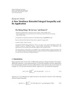
80
100
120
140
160

180
10 20 30 40 50
Number of latent topics
Perplexity
Bigram-PLSA (proposed)
Bigram-PLSA (Nie et al.’s)
Figure 1: The average perplexities obtained by the proposed and
Nie et al.’s bigram-PLSA model with respect to differ ent numbers of
latent topics.
assumed constant and the EM algorithm was employed to
calculate only P(z
l
| w
i
, d
k
) parameters for d
k
= d and
for those w
i
present in the document d. After convergence
of the EM procedure, P(w
j
| w
i
, d) was found. Obtained
matrix P(w
j
| w

i
, d) contained many zero probabilities, thus
we smoothed it using Witten-Bell smoothing method [16].
Note that the folding-in procedure gives the PLSA and the
bigram-PLSA models an unfair advantage by allowing them
to adapt the model parameters to the test data. Nevertheless,
we applied it to avoid overfitting.
To have a valid comparison, the PLSA and Nie et
al.’s bigram-PLSA models were tr ained by the same data
employed to train our proposed bigram-PLSA model. The
folding-in procedure and Witten-Bell smoothing were also
applied on the PLSA and Nie et al.’s bigram-PLSA models.
Figure 1 shows the perplexities of the proposed and Nie et
al.’s bigram-PLSA models for different numbers of latent
topics averaged over ten times of running the experiment.
In this figure, the error bars show the standard errors of the
average perplexities. As seen in Figure 1, the perplexit y of our
proposed bigram-PLSA model is lower than the perplexity
of Nie et al.’s bigram-PLSA model. The best perplexity was
obtained w hen the number of latent topics was set to 40
in both models. Therefore, in the rest of experiments the
numbers of latent topics were set accordingly.
In addition, we performed the paired t-test on the
perplexity results of both methods with the significance level
of 0.01. As stated, each experiment was carried out ten times.
The null hypothesis is whether the average perplexities of two
methods are the same. Tabl e 1 shows the P-value obtained
from the paired t-test for our experiments performed with
different numbers of latent topics. The right column of
Tabl e 1 shows the P-value where the alternative hypothesis

is whether the average perplexity of our method is less
than the average perplexity of Nie et al.’s method. All P-
values obtained are smaller than the specified significance
Table 1: The P-values obtained from the paired t-test on perplexity
results of Nie et al.’s and proposed method for different numbers of
latent topics (K).
KP-value
10 3.58E − 05
20 1.23E
− 07
30 1.23E
− 06
40 4.35E
− 07
50 3.26E
− 08
level. Therefore, the perplexity improvements are statistically
significant.
Tabl e 2 shows the comparison between the average
perplexities of the bigram-PLSA model and other language
models. The standard errors of the average perplexities, the
number of model parameters and the approximate time of
each EM iteration are reported in this table. Note that the
number of model parameters for the bigram and trigram
language models are equal to the number of word pairs
and word triplets observed in the training data, respectively.
The numbers shown in Tabl e 2 are the maximum possible
number of the word pairs and triplets. In this table, the
perplexities of the bigram and trigram language models, the
PLSA model, and linear interpolations of the PLSA model

and the bigram model are also shown. The bigram and
trigram language models were trained by the training data
discussed above and the Katz backoff smoothing method
[17] was applied on them. Stop words and infrequent words
of training data were replaced by #STOP and UNK symbols.
The number of latent topics was set to 40 in the bigram-
PLSA models and 50 in the PLSA model because for the PLSA
model the best perplexity was obtained when the number
of latent topics was set to 50. In case of linear interpolation,
P(w
n
| w
n−1
, d)in(22) was calculated as follows:
P
(
w
n
| w
n−1
, d
)
= λP
bigram
(
w
n
| w
n−1
)

+
(
1
− λ
)
P
PLSA
(
w
n
| d
)
.
(23)
We set λ
= 0.75 in our experiments. This value for λ was
obtained by optimizing it on the held-out data.
As Tab le 2 shows, the proposed bigram-PLSA model
reduces the perplexity more than other language models;
however, the number of parameters and the training time
of the proposed model is more than the other models.
The proposed bigram-PLSA model was incorporated in the
Sphinx 4.0 [18] CSR system and thus evaluated. The SI84
part of Wall Street Journal corpus was used for training the
acoustic models and the November 1992 ARPA CSR test set
was used for testing. The vocabulary contained 5000 words
including 3800 words used for the bigram-PLSA model,
about 200 stop words and about 1000 extra words. We used
aback-off trigram language model trained by the whole
BLLIP WSJ corpus in the decoding process and employed the

PLSA and the bigram-PLSA models for the N-best rescoring.
Since the vocabulary of the bigram-PLSA model contains
only 3800 content words, the stop words and the extra words
existing in the N-best list were replaced by #STOP and UNK
EURASIP Journal on Advances in Signal Processing 7
Table 2: Perplexities, number of parameters, and the computation cost of the bigram-PLSA model and other language models.
Model Calculated parameter
Number of model
parameters
Time of each
EM iteration
Perplexity
bigram P(w
n
| w
n−1
) Maximum 3800
2
— 198
trig ram P(w
n
| w
n−2
w
n−1
) Maximum 3800
3
— 134
PLSA P(w
n

| d) 215000 0.6 second 328 ± 2.1
Bigram & PLSA (linear interpolation) λP(w
n
| w
n−1
)+(1− λ)P(w
n
| d) 14655000 0.6 second 155 ± 6.2
Bigram-PLSA (Nie et al.’s)

L
l
=1
P(w
n
| w
n−1
, z
l
)P(z
l
| d) 577620000 19 minutes 123 ± 4.8
Bigram-PLSA (proposed)

L
l
=1
P(w
n
| w

n−1
, z
l
)P(z
l
| w
n−1
, d) 653600000 24 minutes 101 ± 3.1
Table 3: Average word error rates of the CSR system using PLSA-
based language models with and without t rigram language model
in decoding.
Language Model
(for N-best
rescoring)
WER (%)
(trig ram in
decoding)
WER (%)
(No LM in
decoding)
Average
decoding time
(Sec.)
— 12.66 74.24 0.8
PLSA 11.28
± 0.05 51.73 ± 0.02 4.5
Bigram-PLSA
(Nie et al.’s)
10.65
± 0.04 47.41 ± 0.05 131

Bigram-PLSA
(proposed)
10.28
± 0.02 46.09 ± 0.03 140
Table 4: The P-values obtained from the paired t-test on WER
results of Nie et al.’s and proposed method.
LM in decoding P-value
Trig r am 6.53E − 10
No LM 1.70E
− 10
symbols, respectively. The number of candidates for N-best
rescoring was set to 30 and the number of latent topics was set
to 50 in the PLSA model and 40 in the bigram-PLSA models.
Tabl e 3 shows the word error rates (WERs) of the CSR system
using the PLSA and the bigram-PLSA models averaged over
ten runs of the experiments. In the second column of Table 3,
the trigram language model was used in the decoding process
while in the third column, no language model was used in the
decoding process and only the PLSA-based language models
were used for the N-best rescoring. The standard errors of
average WERs a re also given in this table.
As Table 3 shows, the PLSA and the bigr am-PLSA models
improve the word error rate. In addition, the word error
rate obtained from the bigram-PLSA model is meaningfully
lower than that of the PLSA model. Our proposed bigram-
PLSA model shows slight improvement compared to Nie et
al.’s bigram-PLSA model. The third column better demon-
strates the effect of the bigram-PLSA model in reducing the
word error rate. The average decoding time is given in the
last column of Table 3.ItisobservedthatWERisimproved

for the cost of increasing the decoding time, but the increase
in the decoding time compared to the Nie et al.’s model is
insignificant.
In addition, we performed paired t-test on WER results
of the Nie et al.’s and the proposed methods. The sig nificance
level was set to be 0.01. Ta ble 4 shows the P-values obtained
from the paired t-test. As this table shows, the WER
improvements are statistically significant.
5. Conclusions and Future Work
In this paper, a general framework for combining bigram
and PLSA models was proposed. The combined model was
obtained from incorporating the word history in the PLSA
parameters. Furthermore, the EM procedure for estimating
the parameters of the combined model was described.
Finally, the proposed model was compared to the previous
work done on combining the bigram and the PLSA models
by Nie et al. Our proposed model is different from Nie et
al.’s model in the definition of the topic probability. In Nie
et al.’s model the topic probability is conditioned on the
documents, but in our model, the topic probability is further
conditioned on the bigram history. The proposed model
automatically assigns latent topics to each context word
unevenly in contrast to the even assignment of them by Nie
et al.’s initial bigram-PLSA model. We arranged experiments
to evaluate our combined model based on the perplexity
and the word error rate criteria. Experiments showed that
our proposed bigram-PLSA model outperformed the PLSA
model according to the both criteria. The proposed model
also showed slight superiority over Nie et al.’s big ram-PLSA
model in improving perplexity and WER. As our future

research work, we intend to suggest a similar framework
to combine n-gram and LDA models. We also plan to use
automatic smoothing in our parameter estimation process
without requiring it to be done as an extra step as it is the
state-of-the-art in Bayesian machine learning methods.
Acknowledgment
This paper was in part supported by a grant from Iran
Telecommunication Research Center (ITRC).
References
[1] S. Deerwester, S. Dumais, G. Furnas, T. Landauer, and R.
Harshman, “Indexing by latent semantic analysis,” Journal of
the American Society of Information Science, vol. 41, pp. 391–
407, 1990.
[2] J. R. Bellegarda, “Exploiting latent semantic information in
statistical language modeling,” Proceedings of the IEEE, vol. 88,
no. 8, pp. 1279–1296, 2000.
8 EURASIP Journal on Advances in Signal Processing
[3] T. Hofmann, “Probabilistic latent semantic indexing,” in
Proceedings of the 22nd Annual International ACM SIGIR Con-
ference on Research and Development in Information Retrieval,
pp. 50–57, Berkeley, Calif, USA, 1999.
[4] D. M. Blei, A. Y. Ng, and M. I. Jordan, “Latent Dirichlet
allocation,” Journal of Machine Learning Research, vol. 3, no.
4-5, pp. 993–1022, 2003.
[5] D. Gildea and T. Hofmann, “Topic-based language models
using EM,” in Proceedings of the 6th European Conference on
Speech Communication and Technology (EUROSPEECH ’99),
pp. 235–238, Budapest, Hungary, 1999.
[6] D. Mrva and P. C. Woodland, “Unsupervised language model
adaptation for mandarin broadcast conversation transcrip-

tion,” in Proceedings of International Conference on Spoken
Language Processing, pp. 1549–1552, Pittsburgh, Pa, USA,
2006.
[7] M. Federico, “Language model adaptation through topic
decomposition and MDI estimation,” in Proceedings of Inter-
national Conference on Acoustics, Speech and Signal Processing,
pp. 773–776, Orlando, Fla, USA, 2002.
[8] T. Griffiths, M. Steyvers, D. Blei, and J. Tenenbaum, “Integrat-
ing topics and syntax,” in Advances in Neural Information Pro-
cessing Systems 17, pp. 87–94, Vancouver, Canada, December
2004.
[9] T. L. Griffiths, M. Steyvers, and J. B. Tenenbaum, “Topics in
semantic representation,” Psychological Review, vol. 114, no. 2,
pp. 211–244, 2007.
[10] X. Wang and A. McCallum, “A note on topical n-grams,” Tech.
Rep. UM-CS-2005-071, University of Massachusetts, Amherst,
Mass, USA, December 2005.
[11] M. Girolami and A. Kaban, “Simplicial mixtures of Markov
chains: distributed modeling of dynamic user profiles,” in
Advances in Neural Information Processing Systems 16,pp.9–
16, MIT Press, Vancouver, Canada, December 2003.
[12] H. M. Wallach, “Topic modeling: beyond bag-of-words,” in
Proceedings of the 23rd International Conference on Machine
Learning (ICML ’06), pp. 977–984, Pittsburgh, Pa, USA, June
2006.
[13] J. Nie, R. Li, D. Luo, and X. Wu, “Refine bigram PLSA model
by assigning latent topics unevenly,” in Proceedings of the IEEE
Workshop on Automatic Speech Recognition and Understanding,
pp. 141–146, Kyoto, Japan, 2007.
[14] T. Hofmann, J. Puzicha, and M. I. Jordan, “Learning from

dyadic data,” in Advances in Neural Information Processing
Systems 11, pp. 466–472, Denver, Colo, USA, November-
December 1998.
[15] T. Hofmann, “Unsupervised learning by probabilistic latent
semantic analysis,” Machine Learning, vol. 42, no. 1-2, pp. 177–
196, 2001.
[16] I. H. Witten and T. C. Bell, “The zero-frequency problem:
estimating the probabilities of novel events in adaptive text
compression,” IEEE Transactions on Information Theory, vol.
37, no. 4, pp. 1085–1094, 1991.
[17] S. M. Katz, “Estimation of probabilities from sparse data for
the language model component of speech recognizer,” IEEE
Transactions on Acoustics, Speech, and Signal Processing, vol. 35,
no. 3, pp. 400–401, 1987.
[18] W. Walker, P. Lamere, P. Kwok, et al., “Sphinx-4: a flexible open
source framework for speech recognition,” Tech. Rep. TR2004-
0811, SUN Microsystems, November 2004.