Báo cáo hóa học: " Research Article Advances in Modal Analysis Using a Robust and Multiscale Method" ppt

Hindawi Publishing Corporation
EURASIP Journal on Advances in Signal Processing
Volume 2010, Article ID 392782, 12 pages
doi:10.1155/2010/392782
Research Article
Advances in Modal Analysis Using a Robust and
Multiscale Method
C
´
ecile Picard,
1
Christian Frisson,
2
Franc¸ois Faure,
3
George Drettakis,
1
and Paul G. Kry
4
1
REVES/INRIA, BP 93, 06902 Sophia Antipolis, France
2
TELE Lab, Universit
´
e catholique de Louvain (UCL), 1348 Louvain-la-Neuve, Belgium
3
EVASION/INRIA/LJK, Rh
ˆ
one-Alpes Grenoble, France
4
SOCS, McGill University, Montreal, Canada H3A 2A7

Correspondence should be addressed to C
´
ecile Picard,
Received 1 March 2010; Revised 29 June 2010; Accepted 18 October 2010
Academic Editor: Xavier Serra
Copyright © 2010 C
´
ecile Picard et al. This is an open access article distributed under the Creative Commons Attribution License,
which permits unrestricted use, distribution, and reproduction in any medium, provided the original work is properly cited.
This paper presents a new approach to modal synthesis for rendering sounds of virtual objects. We propose a generic method that
preserves sound variety across the surface of an object at different scales of resolution and for a variety of complex geometries.
The technique performs automatic voxelization of a surface model and automatic tuning of the parameters of hexahedral finite
elements, based on the distribution of material in each cell. The voxelization is performed using a sparse regular grid embedding of
the object, which permits the construction of plausible lower resolution approximations of the modal model. We can compute the
audible impulse response of a v ariety of objects. Our solution is robust and can handle nonmanifold geometries that include both
volumetric and surface parts. We present a system which allows us to manipulate and tune sounding objects in an appropriate way
for games, training simulations, and other interactive virtual environments.
1. Introduction
Our goal is to realistically model sounding objects for
animated realtime virtual environments. To achieve this, we
propose a robust and flexible modal analysis approach that
efficiently extracts modal parameters for plausible sound
synthesis while also focusing on efficient memory usage.
Modal synthesis models the sound of an object as a
combination of damped sinusoids, each of which oscillates
independently of the others. This approach is only accurate
for sounds produced by linear phenomena, but can compute
these sounds in realtime. It requires the computation of a
partial eigenvalue decomposition of the system matrices of
the sounding object, which can be expensive for large com-

plex systems. For this reason, modal analysis is performed
in a preprocessing step. The eigenvalues and eigenvectors
strongly depend on the geometry, material and scale of the
sounding object. In general, complex sounding objects, that
is, with detailed geometries, require a large set of eigenvalues
in order to preserve the sound map, that is, the changes
in sound across the surface of the sounding object. This
processing step can be subject to robustness problems. This
is even more the case for nonmanifold geometries, that is,
geometries where one edge is shared by more than two
faces. Finally, available approaches manage memory usage in
realtime by only pruning part of modal parameters according
to the characteristics of the virtual scene (e.g., foreground
versus background), without specific consideration regard-
ing the objec ts’ sound modelling. Additional flexibility in the
modal analysis itself is thus needed.
We propose a new approach to efficiently extract modal
parameters for any given geometry, overcoming many of the
aforementioned limitations. Our method employs bounding
voxels of a given shape at arbitrary resolution for hexahedral
finite elements. The advantages of this technique are the
automatic voxelization of a surface model and the automatic
tuning of the finite element method (FEM) parameters based
on the distribution of material in each cell. A particular
advantage of this approach is that we can easily deal with
nonmanifold geometry which includes both volumetric and
surface parts (see Section 5). These kinds of geometries
cannot be processed with traditional approaches which use
2 EURASIP Journal on Advances in Signal Processing
a tetrahedralization of the model (e.g., [1]). Likewise, even

with solid watertight geometries, complex details often lead
to poorly shaped tetrahedra and numerical instabilities; by
contrast, our approach does not suffer from this prob-
lem. Our specific contr ibution is the application of the
multiresolution hexahedral embedding technique to modal
analysis for sound synthesis. Most importantly, our solution
preserves variety in what we call the sound map.
The remainder of this paper is organized as foll ows.
RelatedworkispresentedinSection 2. Our method is then
explained in Section 3. A validation is presented in Section 4.
Robustness and multiscale results are discussed in Section 5,
then realtime experimentation is presented in Section 6.We
finally conclude in Section 7.
2. Background
2.1. Related Work. The traditional approach to creating
soundtracks for interactive physically based animations
is to directly playback prerecorded samples, for instance,
synchronized with the contacts reported from a r igid-body
simulation. Due to memory constraints, the number of
samples is limited, leading to repetitive audio. Moreover,
matching sampled sounds to interactive animation is difficult
and often leads to discrepancies between the simulated visu-
als and their accompanying soundtrack. Finally, this method
requires each specific contact interaction to be associated
with a corresponding prerecorded sound, resulting in a time-
consuming authoring process.
Work by Ad rien [2] describes how effec tive digital
sound synthesis can be used to reconstruct the richness of
natural sounds. There has been much work in computer
music [3–5] and computer graphics [1, 6, 7] exploring

methods for generating sound based on physical simula-
tion. Most approaches target sounds emitted by vibrating
solids. Physically based sounds require significantly more
computation power than recorded sounds. Thus, brute-
force sound simulation cannot be used for realtime sound
synthesis. For interactive simulations, a widely used solution
is to apply vibrational parameters obtained through modal
analysis. Modal data can be obtained from simulations [1, 7]
or extracted from recorded sounds of real objects [6]. The
technique presented in this paper is more closely related to
the work of O’Brien et al. [1], which extends modal a nalysis
to objects that are neither simple shapes nor available to be
measured.
The computation time required by current methods to
preprocess the modal analysis prevents it from being used
for realtime rendering. As an example, the actual cost of
computing the partial eigenvalue decomposition using a
tetrahedralization in the case of a bowl with 274 vertices and
generating 2426 tetrahedra is 5 minutes with a 2.26 GHz Intel
Core Duo. Work of Bruyns-Maxwell and Bindel [8] address
interactive sound synthesis and how the change of the shape
of a finite element model affects the sound emission. They
highlight that it is possible to avoid the recomputation of the
synthesis parameters only for moderate changes. There has
been much work in controlling the computational expense
of modal synthesis, allowing the simultaneous handling of a
large variety of sounding objects [9, 10]. However, to be even
more efficient, flexibility should be included in the design of
the model itself, in order to control the processing. Thus,
modal synthesis should be further developed in terms of

parametric control properties. Our technique tackles com-
putational efficiency by proposing a multiscale resolution
approach of modal analysis, managing the amount of modal
data according to memory requirements.
The use of physics engines is becoming much more
widespread for animated interactive virtual environments.
The study from Menzies [11] address the pertinence of
physical audio within physical computer game environment.
He develops a library wh ose technical aspects are based
on practical requirements and points out that the interface
between physics engines and audio has often been one of
the obstacles for the adoption of physically based sound
synthesis in simulations. O’Brien et al. [12] employed
finite elements simulations for generating both animated
videos and audio. However, the method requires large
amounts of computation, and cannot be used for realtime
manipulation.
2.2. Modal Synthesis. Modal sound synthesis is a physically
based approach for modelling the audible vibration modes
of an object. As any kind of additive synthesis, it consists
of describing a source as the sum of many components
[13]. More specifically, the source is viewed as a bank
of damped harmonic oscillators which are excited by an
external stimulus and the modal model is represented with
the vector of the modal frequencies, the vector of the decay
rates and the matrix of the gains for each mode at different
locations on the surface of the object. The frequencies and
dampings of the oscillators are governed by the geometry
and material properties of the object, whereas the coupling
gains of the modes are determined by the mode shapes and

are dependent on the contact location on the object [6].
Modes are computed through an analysis of the govern-
ing equations of motion of the sounding system. The natural
frequencies are determined assuming the dynamic response
of the unloaded structure, with the equation of motion. A
system of n degrees of freedom is governed by a set of n
coupled ordinary differential equations of second order. In
modal analysis, the deformation of the system is assumed to
be a linear combination of normal modes, uncoupling the
equations of motion. The solution for object vibration can
be thus easily computed. To decouple the damped system
into single degree-of freedom oscillators, Rayleigh damping
is generally assumed (see, for instance, [14]).
The response of a system is usually governed by a
relatively small part of the modes, which makes modal
superposition a particularly suitable method for computing
the vibration response. Thus, if the structural response is
characterized by k modes, only k equations need to be solved.
Finally, the initial computational expense in calculating
the modes and frequencies is largely offset by the savings
obtained in the calculation of the response.
Modal synthesis is valid only for linear problems, that
is, simulations with small displacements, linear elastic mate-
rials, and no contact conditions. If the simulation presents
EURASIP Journal on Advances in Signal Processing 3
nonlinearities, significant changes in the natural frequencies
may appear during the analysis. In this case, direct integra-
tion of the dynamic equation of equilibrium is needed, which
requires much more computational effort. For our approach,
the calculations for modal parameters are s imilar to the ones

presentedinthepaperofO’Brienetal.[1].
3. Method
In the case of small elastic deformations, rigid motion of
an object does not interac t with the objects’s vibrations.
On the other hand, we assume that small-amplitude elastic
deformations will not significantly affect the rigid-body
collisions between objects. For these reasons, the rigid-body
behavior of the objects can be modeled in the same way as
animation without audio generation.
3.1. Deformation Model. In most approaches, the deforma-
tion of the sounding object t ypically need to be simulated.
Instead of directly applying classical mechanics to the
continuous system, suitable discrete approximations of the
object geometry can be performed, making the problem
more manageable for mathematical analysis. A variety of
methods could be used, including particle systems [3, 7]
that decompose the structure into small pair-like elements
for solving the mechanics equations, or Boundary Element
Method (BEM) that computes the equations on the surface
(boundary) of the elastic body instead of on its volume (inte-
rior), allowing reflections and diffractions to be modeled [15,
16]. The Finite Element Method (FEM) is commonly used to
perform modal analysis, which in general gives satisfactory
results. Similar to particle systems, FEM discretizes the
actual geometry of the structure using a collection of finite
elements. Each finite element represents a discrete portion
of the physical structure and the finite elements are joined
by shared nodes. The collection of nodes and finite elements
is called a mesh. The tetrahedral finite element method has
been used to apply classical mechanics [1]. However, tetra-

hedral meshes are computationally expensive for complex
geometries, and can be difficult to tune. As an example, in the
tetrahedral mesh generator Tetgen ( />the mesh element quality criterion is based on the minimum
radius-edge ratio, which limits the ratio between the radius
of the circumsphere of the tetrahedron and the shortest edge
length. Based on this observation, we choose a finite elements
approach whose volume mesh does not exactly fit the object.
We use the method of Nesme et al. [17]tomodel
the small linear deformations that are necessary for sound
rendering. In this approach, the object is embedded in a
regular grid where each cell is a finite element, contrary to
traditional FEM models w here the elements try to match
the object geometry as finely as possible. Tuning the grid
resolution allows us to easily trade off accuracy for speed. The
object is embedded in the cells using barycentric coordinates.
Though the geometry of the mesh is quite different from
the object geometry, the mechanical properties (mass and
stiffness) of the cells match as closely as possible the
spatial distribution and the parameters of material. The
technique can be summarized as follows. An automatic
high-resolution voxelization of the geomet ric object is first
built. The voxelization initially concerns the surface of the
geometric model, while the interior is automatically filled
when the geometry represents a solid object. The voxels
are then recursively merged (8 to 1) up to the desired
coarser mechanical resolution. The merged voxels are used
as hexahedral (boxes with the same shape ratio as the fine
voxels) finite elements embedding the detailed geometric
shape. The voxels are usually cubes but the y may have
different sizes in the three directions. At each step of the

coarsification, the stiffness and mass matrices of a coarse
element are computed based on the eight child element
matrices. Mass and stiffness are thus deduced from a fine grid
to a coarser one, where the finest depth is considered close
enough to the surface, and the procedure can be described
as a two-level structure, that is, from fine to coarse grid. The
stiffness and mass matrices are computed bottom-up using
the following equation:
K
parent
=
7

i=0
L
T
i
K
i
L
i
,(1)
where K is the matrix of the parent node, the K
i
are the
matrices in the child nodes, and the L
i
are the interpolation
matrices of the child cell vertices within the parent cell.
Since empty children have null K

i
matrices, the fill rate
is automatically taken into account, as well as the spatial
distribution of the material through the L
i
matrices. As a
result, full cells are heavier and stiffer than partially empty
cells, and the matrices not only encode the fill rate but
also the distribution of the material within each cell. With
this method, we can handle objects with geometries that
simultaneously include volumetric and surface parts; thin or
flat features will occupy voxels and will thus result in the
creation of mechanical elements that robustly approximate
their mechanical behavior (see Section 5.1).
3.2. Modal Analysis. The method for FEM model [17]
is adapted from realtime deformation to modal analysis.
In particular, the modal parameters are extracted in a
preprocessing step by solving the equation of motion for
small linear deformations. We first compute the global mass
and global stiffness matrices for the object by assembling the
element matrices. In the case of three-dimensional objects,
global matrices will have a dimension of 3m
× 3m where
m is the number of nodes in the finite element mesh. Each
entry in each of the 24
× 24 element matrices for a cell
is accumulated into the corresponding entry of the global
matrix. Because each node in the hexahedral mesh shares an
element with only a small number of the other nodes, the
global matrices will be sparse. If we assume the displacements

are small, the discretized system is described on a mechanical
level by the Newton second law
M
¨
d + C
˙
d + Kd
= f,
(2)
where d is the vector of node displacements, and a derivative
with respect to time is indicated by an overdot. M, C,
and K are, respectively, the system’s mass, damping and
4 EURASIP Journal on Advances in Signal Processing
(1) Compute mass and stiffness at desired mechanical level
(2) Assemble the mass and the stiffness matrices
(3) Modal analysis: solve the eigenproblem
(4) Store eigenvalues and eigenvectors for sound synthesis
Algorithm 1: Algorithm for modal parameters extraction.
stiffness mat rices, and f represents external forces, such as
impact forces that will produce audible vibrations. Assuming
Rayleigh damping, that is, C
= α
1
K + α
2
M with some α
1
and α
2
, we can solve the eigenproblem of the decoupled

system leading to the n eigenvalues and the n
× m matrix of
eigenvectors, with n the number of degrees of freedom and m
the number of nodes in the mesh. The sparseness of M and
K matrices allows the use of sparse matrix algorithms for the
eigen decomposition. We refer the reader to Appendices A
and B for more details on the calculation.
Let λ
i
be the ith eigenvalue and φ
i
its corresponding
eigenvector. The eigenvector, also known as the mode shape,
is the deformed shape of the structure as it vibrates in the
ith mode. The natural frequencies and mode shapes of a
structure are used to characterize its dynamic response to
loads in the linear regime. The deformation of the structure
is then calculated from a combination of the mode shapes of
the structure using the modal superposition technique. The
vector of displacements of the model, u,isdefinedas:
u
=

β
i
φ
i
,(3)
where β
i

is the scale factor for mode φ
i
. The eigenvalue for
each mode is determined by the ratio of the mode’s elastic
stiffness to the mode’s mass. For each eigen decomposition,
there will be six zero eigenvalues that correspond to the six
rigid-body modes, that is, modes that do not generate any
elastic forces.
Our preprocessing step that performs modal analysis can
be summarized as in Algorithm 1.
Our model approximates the motion of the embedded
mesh vertices. That is, the visual model with detailed geom-
etry does not match the mechanical model on which the
modal analysis is performed. The motion of the embedding
uses a trilinear interpolation of the mechanical degrees of
freedom, so we can nevertheless compute the motion of any
point on the surface given the mode shapes.
3.3. Sound Generation. In essence, efficiency of modal analy-
sis relies on neg lecting the spatial dynamics and modelling
the actual physical system by a corresponding generalized
mass-spring system which has the same spectral response.
The activation of this model depends on where the object is
hit. If we hit the object at a vibration node of a mode, then
that mode will not vibrate, but others will. This is what we
refer to as the sound map, which could also be called a sound
excitation map as it indicates how the different modes are
excited when the object is struck at different locations.
From the eigenvalues and the matrix of eigenvectors,
we are able to deduce the modal parameters for sound
synthesis. Let λ

i
be the ith eigenvalue and ω
i
its square root.
The absolute value of the imaginary part of ω
i
gives the
natural frequency (in radians/second) of the ith mode of
the structure, whereas the real part of ω
i
gives the mode’s
decay rate. The mode’s gain is deduced from the eigenvectors
matrix and depends on the excitation location. We refer the
reader to the Appendices A and B for more details on modal
superposition.
The sound resulting from an impact on a specific location
j on the surface is calculated as a sum of n damped
oscillators:
s
j
(
t
)
=
n

i=1
a
ij
sin


2πf
i
t

e
−d
i
t
,(4)
where f
i
, d
i
,anda
ij
are, respectively, the frequency, the decay
rate and the gain of the mode i at point j in the sound map.
An object characterized with m mesh nodes and n degrees-
of freedom is described with the vectors of frequencies and
decay rates of dimension n, and the matrix of gains of
dimension n
× m.
3.4. Implementation. Our deformation model implementa-
tion uses the SOFA Framework ( a-framework
.org/) for small elastic deformations. SOFA is an open-source
C++ library for physical simulation and can be used as an
external library in another program, or using one of the
associated GUI applications. This choice was motivated by
the ease with which it could be extended for our purpose.

Regarding sound generation, we synthesize the sounds
via a reson filter (see, for example, Van den Doel et al. [6]).
This choice is made based on the effectiveness for realtime
audio processing. Sound radiation amplitudes of each mode
is also estimated with a far-field radiation model ([15,
Equation (15)]). As the motions of objects are computed
with modal analysis, surfaces can be easily analyzed to
determine how the motions induce acoustic pressure waves
in the surrounding medium. However, we decide to focus
our study on effective modal synthesis. Final ly, our approach
does not consider contact-position-dependent damping or
changes in boundary constraints, as might happen during
moments of excitation. Instead we use a uniform damping
value for the sounding object.
4. Validat ion of the Model
4.1. A Metal Cube. In order to globally validate our method
for modal analysis, we study the sound emitted when
impacting a cube in metal. Due to its symmetry, the cube
should sound the same when struck at any of the eight
corners, with an excitation force whose direction is the same
to the face (see Appendices A and B for more details on
the force amplitude vector). We use a force normal to the
face cube in order to guarantee the maximum energy in all
excited modes. The sound emitted should also be similar
when hitting with perpendicular forces that are both normal
to one pair of the cube faces.
We suppose the cube is made of steel with Young’s
modulus 21
× 10
10

Pa, Poisson ratio 0.33, and densit y
EURASIP Journal on Advances in Signal Processing 5
7850 kg/m
3
. The Raleigh coefficients for stiffness and mass
are set to 1
× 10
−7
and 0, respectively. The use of a constant
damping ratio is a simplification that still produces good
results. The cube model has edges which are 1 meter long.
A Dirac is chosen for the excitation force. In this case, no
radiation properties are considered.
In this example, a 3
× 3 × 3 grid of hexahedral finite
elements is used, leading to 192 modes. However, to adapt
the stiffness of a cell according to its content, the mesh is
refined more precisely than desired for the animation. The
information is propagated from fine cells to coarser cells. For
this example, the elements of the 3
× 3 × 3 cells coarse grid
resolution approximates mechanical properties propagated
from a fine grid of 6
× 6 × 6 cells and 216 elements (see
Section 3.1 for more details on the two-level s tructure).
We observe in Figure 1 that the resulting sounds when
impacting on different corners of the cube are identical. Also,
this is true when exciting with perpendicular forces that are
normal to cube faces. This shows that our model respects the
symmetry of objects, as expected.

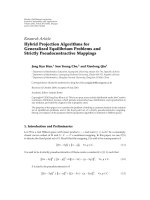
4.2. Position-Dependent Sound Rendering. To pr op er ly re n-
der impact sounds of an object, the method must preserve
the sound variety when hitting the surface at differ ent
locations. We consider a metal bowl, modeled by a triangle
mesh with 274 vertices, shown in Figure 2.
The material of the bowl is aluminium, with the param-
eters 69
× 10
9
Pa for Young’s modulus, 0.33 for Poisson
ratio, and 2700 kg/m
3
for the density. The Rayleigh damping
parameters for stiffness and mass are set to 3
× 10
−6
and 0.01,
respectively. The bowl has a width of 1 meter. No radiation
properties are considered; our study focuses specifically on
modal synthesis.
We compare our approach to modal analysis perfor-
med first using tetrahedralization with Tetgen (http://tetgen
.berlios.de/) with 822 modes. Our method uses hexahedral
finite elements and is applied with a grid of 6
× 6 × 6 cells,
leading to 891 modes. For this example, the elements of the
6
×6×6 cells coarse grid resolution approximates mechanical
properties propagated fr om a fine grid of 12
× 12 × 12 cells.

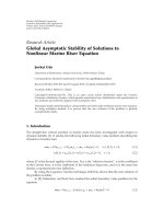
We first compare the extracted modes from both meth-
ods. We observe that the ratio between frequencies a nd
decays is the same for both methods. We then compare the
synthesized sounds from both methods. We take 3 different
locations, that is, top, side and bottom, on the surface of
the object where the object is impacted, see Figure 2.The
excitation force is modeled as a Dirac, such as a regular
impact. The frequency content of the sound resulting from
impact at the 3 locations on the surface is shown in Figure 3.
Each power spectrum is normalized with the maximum
amplitude in order to factor out the magnitude of the impact.
The eigenvalues that correspond to vibration modes will be
nonzero, but for each free body in the system there will be
six zero eigenvalues for the body’s six rigid-body freedoms.
Only the modes with nonzero eigenvalue are kept. Thus,
816 modes are finally used for sound rendering with the
tetrahedralization method and 885 with our hexahedral FEM
method.
Loc 4
Loc 3
Loc 1
Loc 2
(a)
Loc 3
Loc 2
−10
0
−10
2
−10

0
−10
2
−10
0
−10
2
−10
0
−10
2
10
3
10
3
10
3
10
3
Amplitude (dB)
Frequency (Hz)
L
L
o
c
c
2
(b)
Figure 1: A sounding metal cube: sound synthesis is performed for
excitation on 4 different corners and forces n ormal to one pair of

cube faces (a); the power spectrum of the emitted sounds is given
(b).
We provide with the sounds synthesized with the
tetrahedral FEM and the hexadedral FEM approaches (see
additional material ( />Cecile.Picard/Material/AdditionalMaterialEurasip.zip)).
Figure 3 highlights the similarities in the main part of the
frequency content. The difference when impacting at the
bottom (location 3) of the object is due to the difference in
distribution of modes and we believe this is due to the size of
the finite elements used in our method. However, we notice
in listening to the synthesized sounds that those generated
by our method are comparable to those created with the
standard tetrahedralization.
5. Robustness and Multiscale Results
The number of finite elements determine the dimension
of the system to solve. To avoid this expense, we provide
a method that g reatly simplifies the modal parameter
extraction even for nonmanifold geometries. An important
subclass of nonmanifold models are objects that include both
volumetric and surface parts. Our technique consists of using
multiresolution hexahedral embeddings.
6 EURASIP Journal on Advances in Signal Processing
Loc 3
Loc 1
Loc 2
Figure 2: A sounding metal bowl: sound synthesis is performed for
excitation on 3 specific locations on the surface.
5.1. Robustness. Most approaches for tetrahedral mesh
generation have limitations. In particular, an important
requirement imposed by the application of deformable

FEM is that tetrahedra must have appropriate shapes, for
instance, not too flat or sharp. By far the most popular of
the tetrahedr a l meshing techniques are those utilizing the
Delaunay criterion [18]. When the Delaunay criterion is
not satisfied, modal analysis using standard tetrahedraliza-
tion is impossible. In comparison with tetrahedralization
methods, our technique can handle complex geometries and
adequately performs modal analysis. Figures 4 and 5 give an
example of sound modelling on a problematic geometry for
tetrahedralization because of the presence of very thin parts,
specifically the blades that protrude from either side.
We suppose the object is made of aluminum (see
Section 4.2 for the material parameters). The object has a
height of 1 meter. We apply a coarse grid of 7
× 7 × 7cells
for modal analysis. The coarse level encloses the mechanical
properties of a fine grid of 14
× 14 × 14 cells (see Section 3.1
for more details on the two-level structure). In this example,
sound radiation amplitudes of each mode are also estimated
with a far-field radiation model [15, Equation (15)]. Figure 5
shows the power spectrum of the sounds resulting from
impacts, modeled as a Dirac, on 6 different locations. Each
power spectrum is normalized with the maximum amplitude
of the spectrum in order to factor out the magnitude of the
impact.
We provide with the sounds resulting when hitting on the
6different locations (see additional material, link referred in
Section 4.2). Figure 5 shows the variation of impact sounds
at different surface locations due to the sound map since

the different modes have varying amplitude depending on
the location of excitation. The frequency content is related
to the distribution of mass and stiffness along the surface
and more precisely to the ratio between stiffness and mass.
The similarities in the resulting sounds when hitting on
location 1 and location 3 are due to the similarities of the
local geometry. However, the stiffness at location 3 is smaller,
allowing more resonance when being struck which explains
the predominant peak in the corresponding power spectrum.
When hitting the body of the object at location 2, the stiffness
is locally smaller in comparison to locations 1 and 3, leading
to a larger amount of low-frequency content. Also, it is
interesting to examine the quality of the sound rendered
when hitting the wings (locations 4, 5, and 6). Because wings
are thin and light in comparison to the rest of the object, the
higher frequencies are more pronounced. Finally, impacts on
locations 2 and 4 gives comparable sounds since the impact
locations are close on the body of the object.
5.2. A Multi-scale Approach. To study the influence of the
number of hexahedral finite elements on sound rendering,
we model a sounding object with different resolutions of
hexahedral finite elements. We have created a squirrel model
with 999 vertices which we use as our test sounding object.
The squirrel model has a height of 1 meter. Its material is
pine wood, which has parameters 12
× 10
9
Pa for Young’s
modulus, 0.3 for Poisson ratio, and 750 kg/m
3

for the
volumetric mass. Rayleigh damping parameters for stiffness
and mass are set to 8
× 10
−6
and 50, respectively.
Sound synthesis is performed for 3 different locations of
excitation, see Figure 6 (top left). The coarse grid resolution
for finite elements is set to 2
× 2 × 2, 3 × 3 × 3, 5 × 5 × 5, and
7
× 7 × 7. In this example, each grid uses mass and stiffness
computed as described in Section 3.1 from a resolution 4
times finer; that is, the model with resolution 2
× 2 × 2has
properties computed with a grid of 8
× 8 × 8.
We provide with the sounds synthesized with the dif-
ferent grid resolutions for finite elements and for the 3
different locations of excitation (see additional material, link
referred in Section 4.2). Results show that the frequency
content of sounds depend on the location of excitation and
on the resolution of the hexahedral finite elements. The
higher resolution models have a wider range of frequencies
because of the supplementary degrees of freedom. We also
observe a frequency shift as the FEM resolution increases.
Note that a 2
× 2 × 2gridrepresentsanextremelycoarse
embedding, and consequently it is not surprising that the
frequency content is different at higher resolution. Neverthe-

less, there are still some strong similarities at the dominant
frequencies. Above all, a desirable feature is the convergence
of frequency content as the resolution of the model increases.
While additional psychoacoustic experiments with objective
spectral distortion measures would be necessary to validate
this result, when listening to the results, the sound quality for
thismodelatagridof5
× 5 × 5 may produce a convincing
sound rendering for the human ear. Figure 6 suggests that
higher resolutions are necessary before convergence can be
clearly observed in the frequency content. Finally, we note
that the grid resolution required for acceptable precision
in the sound rendering depends on the geometry of the
simulated object.
5.3. Discussion. The sound map is influenced by the resolu-
tion of the hexahedral finite elements. This is related to the
way stiffnesses and masses of different elements are altered
based on their contents. As a consequence, a 2
× 2 × 2
hexahedral FEM resolution would show much less expressive
variation than higher FEM resolution (we refer the reader to
the records provided in the additional material, link referred
in Section 4.2). One approach to improving this would be to
use better approximations of the mass and stiffness of coarse
elements [19].
Modelling numerous complex sounding objects can
rapidly become prohibitively expensive for realtime
EURASIP Journal on Advances in Signal Processing 7
−10
0

−10
2
−10
0
−10
2
Amplitude (dB)
Frequency (Hz)
10
3
10
3
Loc 1
−10
0
−10
2
−10
0
−10
2
Amplitude (dB)
Frequency (Hz)
10
3
10
3
Loc 2
Loc 3
−10

0
−10
2
−10
0
−10
2
Amplitude (dB)
Frequency (Hz)
10
3
10
3
Figure 3: Sound synthesis with a modal approach using classical tetrahedralization with 822 modes (green) and our method with a 6× 6 × 6
hexahedral FEM resolution, leading to 891 modes (blue): power spectrum of the sounds emitted when impacting at the 3 different locations
shown in Figure 2.
Figure 4: An example of a complex geometry that can be handled
with our method. The thin blade causes problems with traditional
tetrahedralization methods.
rendering due to the large set of modal data that has to be
handled. Nevertheless, based on the quality of the resulting
sounds obtained with our method, and given that increased
resolution for the finite elements implies higher memory
and computational requirements for modal data, the FEM
resolution can be adapted to the number of sounding objects
in the virtual scene.
Tabl e 1 gives the computation times and the memory
usage of the modal data, that is, frequencies, decay rates
and gains, when computing the modal analysis with different
FEM resolution on the squirrel model. In this example, the

finer grid resolution is two levels up to the one of coarse grid,
that is, a coarse grid of 2
×2×2 cells has a fine level of 8×8×8
cells with 337 degrees of freedom (3954 for 5
× 5 × 5). These
are computation times of an unoptimized implementation
on a 2.26 GHz Intel Core Duo. We highlight the 5
× 5 × 5
cells resolution since the results indicate that this resolution
may be sufficient to properly render the sound quality of the
object (see Section 5.2). These results could be improved by
reformulating the computations in order to be supported by
graphics processing units (GPU).
Despite the fact that audio is considered a very important
aspect in virtual environments, it is still considered to be of
lower importance than graphics. We believe that physically
modeled audio brings a significant added value in terms
8 EURASIP Journal on Advances in Signal Processing
−10
0
−10
2
−10
0
−10
2
−10
0
−10
2

Amplitude (dB)
10
3
10
3
10
3
Loc 3
Loc 1
Loc 2
Frequency (Hz)
Loc 3
Loc 1
Loc 2
−10
0
−10
2
−10
0
−10
2
−10
0
−10
2
Amplitude (dB)
10
3
10

3
10
3
Loc 4
Loc 5
Loc 6
Frequency (Hz)
Loc 4
Loc 5
Loc 6
Figure 5: The p ower spectrum of the sounds resulting from impacts at the 3 different locations on the body of the object (top) and on the 3
different locations on the wing (bottom). Note that the audible response is different based on where the object is hit.
Table 1: Computation times in seconds and memory usage in
megabytes for different grid resolutions. Computation times are
given for the different steps of the calculation: discretization and
computation of mass and stiffness matrices (T1), eigenvalues
extraction (T2), and gains computation (T3).
Grid Res.
#Modes
T1 T2 T3 Total MEM
(cells) (s) (s) (s) (s) (MB)
7 × 7 × 7 1191 1.81 16.06 3.99 21.89 9.3
6
× 6 × 6 846 0.89 5.78 2.39 9.06 6.8
5
× 5 × 5 579 0.43 2.07 0.97 3.47 4.7
4
× 4 × 4 363 0.24 0.61 0.59 2.88 2.9
3
× 3 × 3 192 0.05 0.14 0.16 0.35 1.6

2
× 2 × 2 81 0.01 0.03 0.01 0.05 0.69
of realism and the increased sense of immersion. Our
method is built on a physically based animation engine, the
SOFA Framework. As a consequence, problems of coherence
between physics simulation and audio are avoided by using
exactly the same model for simulation and sound model ling.
The sound can be processed in realtime knowing the modal
parameters of the sounding object.
6. Exper i menting with the Modal
Sounds in Realtime
To apply excitation signals in realtime to the simulated
sounding objec ts, we implemented an object, or data pro-
cessing block, for Pure Data and Max/MSP, two similar
visual programming modular environments for dataflow
processing. We used the flex t library (o/
Members/thomas/flext/) (API for object development com-
mon to both environments), and the C/C++ code for modal
synthesis of bell sounds from van den Doel and Pai [20]. The
object in use on a Pure Data patch is illustrated in Figure 7).
We provide the user two different ways for the user to interact
with the model. The user can either choose a specific mesh
vertex number of the geometry model (represented in red in
the figure), or can choose a specific location (in green) where
the nearest vertex is deduced by interpolation.
One a dvantage of the method is to give the possibility
to control the parameters of the sounding model in order
EURASIP Journal on Advances in Signal Processing 9
−10
1

−10
0
10
2
−10
2
10
3
Amplitude (dB)
Frequency (Hz)
−10
1
−10
0
10
2
−10
2
10
3
Amplitude (dB)
Frequency (Hz)
−10
1
−10
0
10
2
−10
2

10
3
Amplitude (dB)
Frequency (Hz)
−10
1
−10
0
10
2
−10
2
10
3
Amplitude (dB)
Frequency (Hz)
−10
1
−10
0
10
2
−10
2
10
3
Amplitude (dB)
Frequency (Hz)
−10
1

−10
0
10
2
−10
2
10
3
Amplitude (dB)
Frequency (Hz)
−10
1
−10
0
10
2
−10
2
10
3
Amplitude (dB)
Frequency (Hz)
−10
1
−10
0
10
2
−10
2

10
3
Amplitude (dB)
Frequency (Hz)
−10
1
−10
0
10
2
−10
2
10
3
Amplitude (dB)
Frequency (Hz)
−10
1
−10
0
10
2
−10
2
10
3
Amplitude (dB)
Frequency (Hz)
−10
1

−10
0
10
2
−10
2
10
3
Amplitude (dB)
Frequency (Hz)
−10
1
−10
0
10
2
−10
2
10
3
Amplitude (dB)
Frequency (Hz)
2
× 2 × 2
3
× 3 × 3
5 × 5 × 5
7
× 7 × 7
Resolution

Loc 1
Loc 2 Loc 3
Loc 3
Loc 1
Loc 2
Figure 6: A squirrel in pine wood is sounding when struck at 3 different locations (from left to right). Frequency content of the resulting
sounds with 4 different resolutions for the hexahedral finite elements: (from top to bottom), 2
× 2 × 2, 3 × 3 × 3, 5 × 5 × 5, 7 × 7 × 7cells.
to tune the resulting sounds for the desired effect. For
instance, the size of the geometry can be modified as
different dimensions could be preferred for rendering sounds
in a particular scenario. The mesh geometry is loaded in
Alias
\Wavefront
∗
.obj format, and we use Blender to apply
geometrical transformations in order to test how it affects the
rendering of the resulting sounds.
As our sound model consists of an excitation and a
resonator, interesting sounds can be easily obtained by
convolving modal sounds with user-defined excitations. The
excitation which supplies the energy to the sound system
contributes to a great extent to the fine details of the resulting
sounds. Excitation signals may be produced by various ways:
loading recorded sound samples, using realtime signals
coming from live soundcard inputs, connecting the output
of other audio applications with Pure Data through a sound
server.
This interface can be viewed as a preliminary prototyping
tool for sound design. Indeed, by experimenting sounds with

predefined objects and interactions types, the parameters of
10 EURASIP Journal on Advances in Signal Processing
Load the
MAT file
from SOFA
LoadaWAVfile
a
s excitation
signal
excitation/model
gain factor
Adjust the
volume and
choose the
sound output
pd
I/O
Volume
Modalmat
∼
CEM
ry
rx
rg
point
37.6378
1 10 100 1000
1000 10000010000
2187
.obj

sx
sy
sg
1773
Sound output
dsp
xy z
Launch the GEM windows,
launch the OBJ file, adjust the camera zoom
and choose a vertex or its closest point
pd MAT FILE
pd WAV EXCITATION
pd GEM MODEL
pd GAIN
Set the
ranges
load
load
load
start
stop
trigger
gemwin
number
out of
on: modal
off:wav
output
∼
vertex

camera
zoom
closest
(1)
(2)
(4)
(3)
(5)
Figure 7: Interface for sound design. After having loaded the modal data and the corresponding mesh geometry, the user can experiment
the modal sounds when exciting the object sur face at different locations. Excitation signals may be loaded as recorded sound samples or
realtime tracked from live soundcard inputs.
sounding objects can easily chosen in order to convey specific
sensations in games. Our approach offers a great extent of
control regarding the possibilities of sound modification,
towards a wide audience since its implementation is cross-
platform and open source. In [21], Bruyns proposed an
AudioUnit plugin, that is unfortunately no longer available,
for modal synthesis of arbitrarily shaped objects, where
materials could be changed based on interpolation between
precalculated variations on the model. Lately, Menzies has
introduced VFoley in [22], an opensource environment for
modal synthesis of 3D scenes, with consequent options
on parameterization (particularly with many collision and
surface models), but tied to physically plausible sounds as
opposed to physically-inspired sounds. This is show n in the
movie provided a s additional material (see link referred in
Section 4.2).
7. Conclusion
We propose a new approach to modal analysis using auto-
matic voxelization of a surface model and computation of

the finite elements parameters, based on the distribution of
material in each cell. Our goal is to perform sound rendering
in the context of an animated realtime virtual environment,
which has specific requirements, such as realtime processing
and efficient memory usage.
For simple cases, our method gives results similar to
traditional modal analysis with tetrahedralization. For more
complex cases, our approach provides convincing results.
In particular, sound variety along the object surface, the
sound map, is well preserved. Our technique can handle
complex nonmanifold geomet ries that include both vol-
umetric and surface parts, which cannot be handled by
previous techniques. We are thus able to compute the
audio response of numerous and diverse sounding objects,
such as those used in games, training simulations, and
other interactive virtual environments. Our solution allows
a multiscale solution because the number of hexahedral
finite elements only loosely depends on the geometry of
the sounding object. Finally, since our method is built on a
physics animation engine, the SOFA Framework,problems
of coherence between simulation and audio can be easily
addressed, which is of great interest in the context of
interactive environment.
In addition, due to the fast computation time, we are
hopeful that realtime modal analysis will soon be possible
on the fly, with sound results that are approximate but still
realistic for virtual environments. For this purpose, psychoa-
coustic experiments should be conducted to determine the
resolution level for acceptable quality of the sound rendering.
Appendices

These appendices give the mathematical background behind
modal superposition for discrete systems with proportional
damping. To apply modal superposition, we assume the
steady state situation, that is, the sustained part of the
impulse response of an object being struck. Indeed, the
early part, which is of very short duration, contains many
frequencies and is consequently not well described by a
discrete set of frequencies. Modal superposition uses the
EURASIP Journal on Advances in Signal Processing 11
Finite Element Method (FEM) and determine the impulse
response of vibrating objects by means of a superposition of
eigenmodes.
A. Derivation of the Equations
We first consider the undamped system; its equation of
motion is expressed by
M
¨
x + Kx
= f
,(A.1)
where M and K are, respectively, the mass and stiffness
matrices of the discrete system. The mass matrix is typically
a diagonal matrix, its main diagonal being populated with
elements whose value is the mass assumed in each degree of
freedom (DOF). The stiffness matrix is sy mmetric (often a
sparse matrix, that is, only a band of elements around the
main diagonal is populated and the other elements are zero).
In finite elements, these matrices are assembled based on the
element geometry and properties.
Since the study is in the frequency domain, the displace-

ment vector x and the force vector f are based on harmonic
components, that is, x
= Xe
jωt
,
˙
x = jωXe
jωt
,
¨
x =−ω
2
Xe
jωt
and f = Fe
jωt
. X and F are two amplitude vectors and contain
oneelementforeachdegreeoffreedom(DOF).Theelements
of X are the displacement amplitudes of the respective DOF
as a funct ion of ω and the elements of F are the amplitudes
of the force, again depending on ω, acting at location and in
direction of the corresponding DOF. Since the harmonic part
is available on both sides, we can ignore it and the equation
of motion can be rewritten
X
=

K − ω
2
M


−1
F
,(A.2)
where X and F means in practice X( ω)andF(ω), but
are shorten for simplification, and ω is a diagonal matrix.
Equation (A.2) is the direct frequency response analysis. The
term K
− ω
2
M needs to be calculated for each frequency. To
calculate the response to any excitation force F(ω), we need
to solve the eigenvalue problem:

K − ω
2
M

X = 0,
(A.3)
or

M
−1
K

X = ω
2
X = λX.
(A.4)

This equation says that each sounding object has a struc ture-
related set of eigenvalues λ, which are simply connected to the
system’s frequencies. To extract the eigenvalues, the following
condition has to be fulfilled
det

K − ω
2
M

=
0
. (A.5)
Solving (A.5) implies finding the roots of a polynomial,
which correspond to the eigenvalues λ. The latter can then
be replaced in (A.3):
(
K
− λM
)
Ψ = 0,
(A.6)
Ψ is the matrix of eigenvectors, or eigenfunc tions, where
the column r is the vector related to the eigenvalue ω
2
r
.
The eigenvectors define the mode shapes linked to the
corresponding frequency of the system.
If the frequencies are unique, many eigenvectors can be

extracted for a given eigenvalue and all are proportional.
Thus, the information enclosed in the eigenvectors is not the
absolute amplitude but a ratio between the amplitudes in the
degrees of freedom. For this reason, the eigenvectors are often
normalized according to a reference. Due to the orthogonal
property of the eigenvectors, Ψ
T
Ψ = I. Consequently, Ψ
T
MΨ
and Ψ
T
KΨ are diagonal matrices, and are, respectively, called
the modal mass and the modal stiffness of the system,
because the ratio between modal stiffness and modal mass
gives the matrix of eigenvalues. A very suitable reference
choice is to scale the eigenvectors so that the modal mass
matrix becomes an identity matrix. From (A.2), we can write:
Ψ
T

K − ω
2
M

Ψ = Ψ
T
F
(
ω

)
X
(
ω
)
Ψ,

λ − ω
2
I

=
Ψ
T
F
(
ω
)
X
(
ω
)
Ψ,
(A.7)
and finally
X
(
ω
)
= Ψ


λ − ω
2
I

−1
Ψ
T
F
(
ω
)
. (A.8)
Equation (A.8) simply expresses that the response X(ω)can
be calculated by surimposing a set of eigenmodes weighted
by the excitation frequency, multiplied with an excitation
load vector F(ω).
Properties of Eigenvalues and Eigenvectors. The orthogonality
of modes expresses that each mode contains information
which the other modes do not have, and consequently a given
mode cannot be built from the others. On the other hand,
solutions of geometrically symmetric systems often give pairs
of multiple eigenmodes.
Boundary conditions are settled simply by prescribing
the value of certain degrees of freedom resolved in the
displacement vector. As an example, a structure rigidly
attached to the ground will show null DOFs around the
support point. Consequently, the elements in the mode
shapes corresponding to these DOFs will always be zero and
will not need to be solved.

B. Damping
We now consider a damped system, and in particular
the proportional damping model which assumes that the
damping can be expressed proportional to the stiffness and
mass matrix (Raleigh damping), that is, C
= α
1
K + α
2
M.
In consequence, the eigenvalues of the proportional damped
system are complex and can be expressed according to the
eigenvalues of the undamped case
λ

r
= ω
2
r

1+ jη
r

,(B.1)
where the imaginary part contains the loss factor η
r
.
Themodalsuperpositionisthusgivenby
X
(

ω
)
= Ψ

λ − ω
2
I + jηλ

−1
Ψ
T
F
(
ω
)
.
(B.2)
12 EURASIP Journal on Advances in Signal Processing
Equation (B.2) enables us to determine entire response
velocity fields that cause the surrounding medium to vibrate
and to generate sound.
Acknowledgments
ThisworkwaspartlyfundedbyEdenGames(http://www
.eden-games.com/), an ATAR I Game Studio in Lyon, France.
C. Frisson is supported by numediart (edi-
art.org/), a long-term research program centered on digital
media arts, funded by R
´
egion Wallonne, Belgium (Grant no.
716631). The authors would like to thank Nicolas Tsingos

for his input on an early draft. Special thanks to Micha
¨
el
Adam and Florent Falipou for their expertise in the SOFA
Framework.
References
[1] J. F. O’Brien, C. Shen, and C. M. Gatchalian, “Synthesizing
sounds from rigid-body simulations,” in Proceedings of ASM
SIGGRAPH Symposium on Computer Animation, pp. 175–181,
July 2002.
[2] J M. Adrien, “The missing link: modal synthesis,” in Represen-
tations of Musical Signals, pp. 269–298, MIT Press, Cambridge,
Mass, USA, 1991.
[3] C. Cadoz, A. Luciani, and J. Florens, “Responsive input
devices and sound synthesis by simulation of instrumental
mechanisms: the CORDIS system,” Computer Music Journal,
vol. 8, no. 3, pp. 60–73, 1984.
[4]F.Iovino,R.Causs
´
e, and R. Dudas, “Recent work around
modalys and modal synthesis,” in Proceedings of the Interna-
tional Computer Music Conference (ICMC ’97), pp. 356–359,
1997.
[5] P.R.Cook,Real Sound Synthesis for Interactive Applications,A.
K. Peters, 2002.
[6] K. Van den Doel, P. G. Kry, and D. K. Pai, “Foley automatic:
physically-based sound effects for interactive simulation and
animation,” in Proceedings of the Computer Graphics Annual
Conference (SIGGRAPH ’01), pp. 537–544, August 2001.
[7] N. Raghuvanshi and M. C. Lin, “Interactive sound synthesis

for large scale environments,” in Proceedings of ACM SIG-
GRAPH Symposium on Interactive 3D Graphics and Games
(I3d ’06), pp. 101–108, March 2006.
[8] C. Bruyns-Maxwell and D. Bindel, “Modal parameter tracking
for shape-changing geometric objects,” in Proceedings of
the 10th International Conference on Digital Audio Effects
(DAFx ’07), 2007.
[9] Q. Zhang, L. Ye, and Z. Pan, “Physically-based sound synthesis
on GPUs,” in Proceedings of the 4th International Conference
on Entertainment Computing, vol. 3711 of Lecture Notes in
Computer Scie nce, pp. 328–333, 2005.
[10] N. Bonneel, G. Drettakis, N. Tsingos, I. Viaud-Delrnon,
and D. James, “Fast modal sounds with scalable frequency-
domain synthesis,” in Proceeding of ACM International Con-
ference on Computer Graphics and Interactive Techniques
(SIGGRAPH ’08), August 2008.
[11] D. Menzies, “Physical audio for virtual environments, phya
in review,” in Proceedings of the International Conference on
Auditory Display (ICAD), G. P. Scavone, Ed., pp. 197–202,
Schulich School of Music, McGill University, 2007.
[12] J. F. O’Brien, P. R. Cook, and G. Essl, “Synthesizing sounds
from physically based motion,” in Proceedings of the ACM
SIGGRAPH Conference on Computer Graphics, pp. 529–536,
Los Angeles, Calif, USA, August 2001.
[13] R. J. McAulay and T. F. Quatieri, “Speech analysis/ synthesis
based on a sinusoidal representation,” IEEE Transactions on
Acoustics, Speech and Signal Processing, vol. 34, no. 4, pp. 744–
754, 1986.
[14] K J. Bathe, Finite Element Procedures in Engineering Analysis,
Prentice-Hall, Englewood Cliffs, NJ, USA, 1982.

[15] D. L. James, J. Barbi
ˇ
c,andD.K.Pai,“Precomputedacoustic
transfer: output-sensitive, accurate sound generation for geo-
metrically complex vibration sources,” ACM T ransactions on
Graphics, vol. 25, no. 3, pp. 987–995, 2006.
[16] J.N.Chadwick,S.S.An,andD.L.James,“Harmonicshells:a
practical nonlinear sound model for near-rigid thin shells,” in
Proceedings of ACM Transactions on Graphics, 2009.
[17] M. Nesme, Y. Payan, and F. Faure, “Animating shapes at arbi-
trary resolution with non-uniform sti
ffness,” in Proceedings
of Eurographics Workshop in Virtual Reality Interaction and
Physical Simulation (VRIPHYS ’06), 2006.
[18] J. R. Shewchuk, “A condition guaranteeing the existence of
higher-dimensional constrained Delaunay triangulations,” in
Proceedings of the 14th Annual Symposium on Computational
Geometry, pp. 76–85, June 1998.
[19] M. Nesme, P. G. Kry, L. Je
ˇ
r
´
abkov
´
a, and F. Faure, “Preserving
topology and elasticity for embedded deformable models,”
ACM Transactions on Graphics,vol.28,no.3,articleno.52,
2009.
[20] K. van den Doel and D. K. Pai, “Modal Synthesis for Vibrating
Objects,” in Audio Anecdotes III: Tools, Tips, and Techniques for

Digital Audio, pp. 99–120, A. K. Peter, 3rd e dition, 2006.
[21] C. Bruyns, “Modal synthesis for arbitrarily shaped objects,”
Computer Music Journal, vol. 30, no. 3, pp. 22–37, 2006.
[22] D. Menzies, “Phya and vfoley, physically motivated audio
for virtual environments,” in Proceedings of the 35th AES
International Conference, 2009.