Báo cáo hóa học: " Research Article Time-Frequency-Based Speech Regions Characterization and Eigenvalue Decomposition Applied to Speech Watermarking" pptx

Hindawi Publishing Corporation
EURASIP Journal on Advances in Signal Processing
Volume 2010, Article ID 572748, 10 pages
doi:10.1155/2010/572748
Research Article
Time-Frequency-Based Speech Regions Characterization and
Eigenvalue Decomposition Applied to Speech Watermarking
Irena Orovi
´
c and Srdjan Stankovi
´
c
Faculty of Electrical Eng ineering, University of Montenegro, 81000 Podgorica, Montenegro
Correspondence should be addressed to Irena Orovi
´
c,
Received 13 February 2010; Revised 21 June 2010; Accepted 30 July 2010
Academic Editor: Bijan Mobasseri
Copyright © 2010 I. Orovi
´
c and S. Stankovi
´
c. This is an open access article distributed under the Creative Commons Attribution
License, which permits unrestricted use, distribution, and reproduction in any medium, provided the original work is properly
cited.
The eigenvalues decomposition based on the S-method is employed to extract the specific time-frequency characteristics of speech
signals. This approach is used to create a flexible speech watermark, shaped according to the time-frequency characteristics of the
host signal. Also, the Hermite projection method is applied for characterization of speech regions. Namely, time-frequency regions
that contain voiced components are selected for watermarking. The watermark detection is performed in the time-frequency
domain as well. The theory is tested on several examples.
1. Introduction

Digital watermarking has been developed to provide efficient
solutions for ownership protection, copyright protection,
and authentication of digital multimedia data by embedding
a secret signal called the watermark into the cover media.
Depending on the applications, two watermarking scenarios
are available: robust and fragile. The robust watermarking
assumes that the watermark should be resistant to various
signal processing techniques called attacks. At the same
time, the watermark should be imperceptible. In order
to meet these requirements, a number of watermarking
techniques have been proposed, many of which are related
to speech and audio signals [1–11]. One of the earliest and
simplest techniques is based on the LSB coding [1–4]. The
watermark embedding is done by altering the individual
audio samples represented by 16 bits per sample. The human
auditory system is sensitive to the noise introduced by
LSB replacement, which limits the number of LSBs that
can be imperceptibly modified. The main disadvantage of
these methods is their low robustness [1]. In a number
of watermarking algorithms, the spread-spectrum technique
has been employed [5–7]. The spread spectrum sequence can
be embedded in the time domain, FFT coefficients, cepstral
coefficients, and so forth. The embedding is performed in
a way to provide robustness to common attacks (noise,
compression, etc.). Furthermore, several algorithms use the
phase of audio signal for watermarking, such are the phase
coding and phase modulation approaches [8, 9], assuring
good imperceptibility. Namely, imperceptible phase modi-
fications are exploited by the controlled phase alternation
of the host signal. However, the fact that they are nonblind

watermarking methods (the presence of the original signal is
required for watermark detection) limits the number of their
applications.
Most of existing watermarking techniques are based
on either the time domain or the frequency domain. In
both cases, the changes in the signal may decrease the
subjective quality, since the time-frequency characteristics
of the watermark do not correspond to the time-frequency
characteristics of the host signal. This may cause water-
mark audibility because it will be present in the time-
frequency regions where speech components do not exist.
In order to adjust the location and the strength of the
watermark to the time-varying spectral content of the
host signal, a time-frequency domain-based approach is
proposed in this paper. The watermark, shaped in accor-
dance with the formants in the time-frequency domain,
will be more imperceptible and more robust at the same
time.
2 EURASIP Journal on Advances in Signal Processing
The time-frequency distributions have been used to char-
acterize the time-varying spectral content of nonstationary
signals [12–16]. As the most commonly used, the Wigner
distribution can provide an ideal representation for linear
frequency-modulated monocomponent signals [12, 15]. For
multicomponents signals, the S-method, that is, a cross-
terms-free Wigner distribution, can be used [16]. The S-
method can be also used to separate the signal components.
Note that the signal components separation could be of
interest in many applications. In particular, in watermarking
it allows creating the watermark that is shaped by using

an arbitrary combination of the signal components. The
eigenvalues-based S-method decomposition is applied to
separate the signal components [17, 18].
In order to provide suitable compromise between imper-
ceptibility and robustness, the watermark should be shaped
according to the time-frequency components of speech sig-
nal, as proposed in [19, 20]. Therein, the speech components
selection is performed by using the time-frequency support
function with a certain energy threshold. However, the
threshold is chosen empirically and it does not provide
sufficient flexibility. Namely, it includes all components
with the energy between the maximum and the threshold
level.
Therefore, in this paper, the eigenvalue decomposition
method is employed to create a time-frequency mask as an
arbitrary combination of speech components (formants).
Only the components from voiced time-frequency regions
are considered [19]. The Hermite projection method-based
procedure for regions characterization is applied[21, 22].
The speech regions are reconstructed within the time-
frequency plane by using a certain number of Hermite
expansion coefficients. The mean square error between the
original and reconstructed region is used to characterize
dynamics of regions. It allows distinguishing between voiced,
unvoiced, and noisy regions. Finally, the watermark embed-
ding and detection are performed in the time-frequency
domain.Therobustnessoftheproposedprocedureisproved
under various common attacks.
The considered watermarking approach can be useful
in numerous applications assuming speech signals. These

applications include, but are not limited to, the intellectual
property rights, such as proof of ownership, speaker verifi-
cation systems, VoIP, and mobile applications such as cell-
phone tracking. Recently, an interesting application of speech
watermarking has appeared in air trafficcontrol[11]. The
air traffic control relies on voice communication between
the aircraft pilot and air traffic control operators. Thus,
the embedded digital information can be used for aircraft
identification.
The paper is organized as follows. A theoretical back-
ground on the time-frequency analysis is given in Section 2.
Section 3 describes the speech regions characterization pro-
cedure. In Section 4, the formants selection based on the
eigenvalues decomposition is proposed. The time-frequency-
based watermarking procedure is presented in Section 5.
The performance of the proposed procedure is tested on
examples in Section 6. Concluding remarks are given in
Section 7.
2. Theoretical Background—Time-Frequency
Analysis
The simplest time-frequency distribution is the spectrogram.
It is defined as a square module of the short-time Fourier
transform (STFT) [15]:
SPEC
(
t, ω
)
=|STFT(t, ω)|
2
=






∞
−∞
x
(
t + τ
)
w
(
τ
)
e
−jωτ
dτ




2
,
(1)
where x(t) is a signal while w(t) is a window function.
The time-frequency resolution in spectrogram depends
on the window function w(t) (window shape and window
width). Namely, if the signal phase is not linear, it cannot
simultaneously provide a good time and frequency resolu-

tion. Various quadratic distributions have been introduced
to improve the spectrogram resolution. Among them, the
most commonly used, [1, 14, 15], is the Wigner distribution,
defined as follows:
WD
(
t, ω
)
=

∞
−∞
x

t +
τ
2

x
∗

t −
τ
2

e
−jωτ
dτ. (2)
However, for multicomponent signals the Wigner dis-
tribution produces a large amount of cross-terms. The S-

method has been introduced to reduce or remove the cross-
terms while keeping the autoterms concentration as in the
Wigner distribution [16]:
SM
(
t, ω
)
=

∞
−∞
P
(
θ
)
STFT
(
t, ω + θ
)
STFT
∗
(
t, ω
− θ
)
dθ.
(3)
A finite frequency domain window is denoted as P(θ). Note
that, for P(θ)
= 2πδ(θ)andP(θ) = 1, the spectrogram and

the pseudo-Wigner distribution are obtained, respectively.
By taking the rectangular frequency domain window, the
discrete form of the S-method can be written as follows:
SM
(
n, k
)
=
L

l=−L
P
(
l
)
STFT
(
n, k + l
)
STFT
∗
(
n, k
− l
)
=|STFT
(
n, k
)
|

2
+2Real
⎧
⎨
⎩
L

l=1
STFT
(
n, k + l
)
STFT
∗
(
n, k
− l
)
⎫
⎬
⎭
,
(4)
where n and k are discrete time and frequency samples. If
the minimal distance between autoterms is greater than the
window width (2L + 1), the cross-terms will be completely
removed. Also, if the autoterms width is equal to (2L +1),
the S-method produces the same autoterms concentration
as the Wigner distribution. Moreover, since the convergence
within P(l) is fast, in many practical applications a good

concentration can be achieved by setting L
= 3.
The advantages of time-frequency representations have
also been used to provide an efficient time-varying filtering.
EURASIP Journal on Advances in Signal Processing 3
The output of the time-varying filter is defined as follows
[23]:
Hx
(
t
)
=
1
2π

∞
−∞
L
H
(
t, ω
)
STFT
x
(
t, ω
)
dω,(5)
where L
H

(t, ω)is a space-varying transfer function (i.e.,
support function) which is defined as Weyl symbol mapping
of the impulse response into the time-frequency domain.
Assuming that the signal components are located within the
time-frequency region R
f
, the support function L
H
(t, ω)can
be defined as follows:
L
H
(
t, ω
)
=
⎧
⎨
⎩
1, for
(
t, ω
)
∈ R
f
,
0, for
(
t, ω
)

/
∈R
f
.
(6)
Although it was initially introduced for signal denoising,
the concept of nonstationary filtering can be used to
retrieve the signal with specific characteristics from the time-
frequency domain.
Therefore, the time-frequency analysis can provide com-
plete information about the time-varying spectral compo-
nents, even when their number is significant as in the
case of speech signals. Namely, these components appear
in the time-frequency plane as recognizable time-varying
structures that could be used to characterize different speech
regions (voiced, unvoiced, noisy, etc.), as proposed in the
sequel. Furthermore, the extraction of individual speech
components from the time-frequency domain could be
useful in many applications assuming speech signals. This
is generally a highly demanding task due to the number of
speech components. As an effective solution, a method based
on the eigenvalues decomposition and the speech signal
time-frequency representation is presented in Section 4.
3. Speech Regions Characterization by
Using the Fast Hermite Projection Method of
Time-Frequency Representation
3.1. Fast Hermite Projection Method. The fast Hermite pro-
jection method has been introduced for image expansion
into a Fourier series by using an orthonormal system of
Hermite functions [21, 22]. Namely, the Hermite functions

provide better computational localization in both the spa-
tial and the transform domain, in comparison with the
trigonometric functions. The Hermite projection method
has been mainly used in image processing applications, such
as image filtering, and texture analysis. Here, we provide a
brief overview of the method.
The ith order Hermite function is defined as follows:
ψ
i
(
x
)
=
(
−1
)
i
e
x
2
/2

2
i
i!
√
π
·
d
i


e
−x
2

dx
i
. (7)
Generally, the Hermite projection method for two-
dimensional signal f (x,y) can be defined as follows:
F

x, y

=
∞

i=0
∞

j=0
c
ij
ψ
ij

x, y

,(8)
where ψ

ij
(x, y)are the two-dimensional Hermite functions
while c
ij
=

∞
−∞

∞
−∞
f (x, y)ψ
ij
(x, y)dx dy are the Hermite
coefficients.
In our case, the two-dimensional function f (x,y)isa
time-frequency representation of a speech region, which will
be represented by a certain number of Hermite coefficients
c
ij
. Note that the number of coefficients c
ij
depends on
the number of the employed Hermite functions. The more
functions is used, the less error is introduced in the
reconstructed version F(x,y).
However, for the sake of simplicity, the expansion can
be performed even along one dimension only. Thus, the
decomposition into N Hermite functions can be defined as
follows:

F
y
(
x
)
=
N−1

i=0
c
i
ψ
i
(
x
)
,(9)
where F
y
(x) = F(x, y)holdsforafixedy while the
coefficients of the Hermite expansion are obtained as follows:
c
i
=

∞
−∞
f
y
(

x
)
ψ
i
(
x
)
dx. (10)
Accordingly, the functions f
y
(x) correspond to the rows
of the time-frequency representation.
The Hermite coefficients could also be defined by using
the Hermite polynomials as follows:
c
i
=
1

2
i
i!
√
π

∞
−∞
e
−x
2


f
(
x
)
e
x
2

H
i
(
x
)
dx, (11)
where
H
i
(
x
)
=
(
−1
)
i
e
x
2
d

i

e
−x
2

dx
i
, (12)
is the Hermite polynomial. Thus, the calculation of the
Hermite coefficients could be approximated by the Gauss-
Hermite quadrature:
c
i
=
1

2
i
i!
√
π
M

m=1
A
m

f
(

x
m
)
e
(x
2
m
/2)

H
i
(
x
m
)
, (13)
where x
m
are zeros of Hermite polynomials while A
m
=
2
M−1
M!
√
π/(M
2
H
2
M

−1
(x
m
)) are associated weights.
By using Hermite functions instead of Hermite polyno-
mials, the following simplified expression is obtained:
c
i
(
x
)
≈
1
M
M

m=1
μ
i
M
−1
(
x
m
)
f
(
x
m
)

. (14)
The constants μ
i
M
−1
(x
m
)are obtained by
μ
i
M
−1
(
x
m
)
=
ψ
i
(
x
m
)

ψ
M−1
(
x
m
)


2
. (15)
4 EURASIP Journal on Advances in Signal Processing
123456 7 8910111213141516171819
1000 2000 3000 4000 5000 6000 7000 8000
50
100
150
200
250
(a)
20 21 22 23 24
1000 2000 3000 4000 5000 6000 7000 8000 9000 10000
50
100
150
200
250
(b)
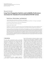
Figure 1: Illustration of various regions within the speech signal.
3.2. Speech Regions Characterization by Using the Concept of
Hermite Projection Method. According to (8) or its simplified
form (9), the time-frequency representation of a speech
region as a two-dimensional function can be expanded
into a certain number of Hermite functions. Thus, we may
assume that f (x, y)
= D(t, ω)andF(x, y) = D
r
(t, ω),

where D denotes the original time-frequency region and
D
r
is the region reconstructed from the Hermite expansion
coefficients. The difference between D and D
r
will depend on
the number of Hermite functions used for the expansion, as
well as on the complexity of the considered region.
The S-method is used for time-frequency representation
of speech signals. By observing time-frequency character-
istics, a significant difference between noise, pauses, and
speech can be noted. Moreover, the voiced and unvoiced
speech parts are significantly different. The voiced parts are
characterized by higher energy and complex structure.
Let us consider different regions of speech signal having
different structure complexity. The fast Hermite projection
method is applied to these regions. By using a small number
of Hermite functions, a certain error will be intentionally
produced. The regions with simpler structures will have
smaller errors, and vise versa. The mean square errors are
calculated as follows:
MSE
(
i
)
=
1
d
1

d
2

t

ω

D
i
(
t, ω
)
− D
r
i
(
t, ω
)

, (16)
where D
i
(t,ω)andD
r
i
(t, ω) denote the original and the
reconstructed ith region from SM(t, ω) while d
1
and d
2

are dimensions of the regions. Thus, the region D
r
i
(t, ω),
containing either noise or unvoiced sounds, will produce
a significantly lower MSE than the region D
r
i
(t, ω)with
complex voiced structures. The dimensions d
1
and d
2
are the
same for all regions. They are chosen experimentally such
that the region includes most of the sound components.
Table 1: MSEs for some of the tested speech regions.
No. Region description MSE
1Noise3∗10
−4
2Noise3∗10
−5
3Noise1∗10
−4
4Noise1∗10
−6
5Noise4∗10
−7
6Noise6∗10
−7

7Noise5∗10
−4
8 Voiced 9971
9 Voiced 2265
10 Voiced 5917
11 Voiced 16587
12 Voiced 5245
13 Unvoiced 55
14 Voiced 4466
15 Voiced 3242
16 Unvoiced 606
17 Voiced 19016
18 Voiced 23733
19 Voiced 7398
20 Unvoiced 0.018
21 Unvoiced 1.25
22 Unvoiced 0.007
23 Unvoiced 0.049
24 Unvoiced 4.38
An illustration of various regions within a speech signal
is given in Figure 1. The MSEs are presented in Tabl e 1
(ten Hermite functions have been used). It can be observed
that the noisy regions (without speech components) have
MSEs below 10
−3
while the regions containing complex
formant structures have a large value of MSE (generally, it is
significantly above 10
3
). The MSEs for the unvoiced regions

are between the two cases.
Therefore, based on the numerous experiments, the
voiced regions with emphatic formants are determined by
MSE > 2
∗ 10
3
. These regions have a rich formants
structure and they will be appropriate for watermarking. A
set of arbitrary selected formants could be used to shape
the watermark. It will provide a flexibility to create the
watermark with very specific time-frequency characteristics.
The combination of time-frequency components could be an
additional secret key to increase robustness and security of
this procedure.
4. Eigenvalue Decomposition Based on
the Time-Frequency Distribution
The S-method produces a representation that is equal to or
very close approximates the sum of the Wigner distribu-
tions calculated for each signal component separately. This
property is used to introduce the eigenvalue decomposition
EURASIP Journal on Advances in Signal Processing 5
method. Let us start from the discrete form of the Wigner
distribution
WD
(
n, k
)
=
N/2


m=−N/2
x
(
n + m
)
x
∗
(
n
− m
)
e
−j(2π/N+1)2mk
,
(17)
where m is a discrete lag coordinate. Consequently, the
inverse of the Wigner distribution can be written as follows:
x
(
n
1
)
x
∗
(
n
2
)
=
1

N +1
N/2

k=−N/2
WD

n
1
+ n
2
2
, k

e
j(2π/N+1)k(n
1
−n
2
)
,
(18)
where n
1
= n + m and n
2
= n − m. Furthermore, for
a multicomponent signal, x(n)
=

M

i
=1
x
i
(n), (18)canbe
written as follows [17, 18]:
M

i=1
x
i
(
n
1
)
x
∗
i
(
n
2
)
=
1
N +1
N/2

k=−N/2
M


i=1
WD
i

n
1
+ n
2
2
, k

×
e
j(2π/N+1)k(n
1
−n
2
)
.
(19)
Having in mind that the S-method is SM(n, k)
=

M
i=1
WD
i
(n, k), the previous equation can be written as
follows:
M


i=1
x
i
(
n
1
)
x
∗
i
(
n
2
)
=
1
N +1
N/2

k=−N/2
SM

n
1
+ n
2
2
, k


e
j(2π/N+1)k(n
1
−n
2
)
.
(20)
By introducing the following notation:
R
SM
(
n
1
, n
2
)
=
1
N +1
N/2

k=−N/2
SM

n
1
+ n
2
2

, k

e
j(2π/N+1)k(n
1
−n
2
)
,
(21)
we have
R
SM
(
n
1
, n
2
)
=
M

i=1
x
i
(
n
1
)
x

∗
i
(
n
2
)
. (22)
The eigenvalue decomposition of the matrix R
SM
is defined
as follows [17, 18]:
R
SM
=
N+1

i=1
λ
i
v
i
(
n
)
v
∗
i
(
n
)

, (23)
where λ
i
are eigenvalues and v
i
(n)areeigenvectorsofR
SM
.
Furthermore, λ
i
= E
f
i
, i = 1, , M (E
f
i
is the energy of the
ith component), and λ
i
= 0fori = M +1, , N, that is,
λ
i
=
M

l=1
E
f
l
δ

(
i − l
)
, (24)
where δ(i) denotes the Kronecker symbol.
As it will be explained in the sequel, the autocorrelation
matrix R
SM
(n
1
, n
2
) is calculated according to (21)foreach
time-frequency region SM(n, k)(obtained by using the S-
method). Then, the eigenvalue decomposition is applied
to R
SM
according to (23), resulting in eigenvalues and
eigenvectors. Each of these components is characterized by
a certain location in the time-frequency plane.
Once separated, they could be further combined in
various ways to provide an arbitrary time-frequency map
used as a support function in watermark modelling.
4.1. Selection of Speech Formants Suitable for Watermarking.
After the regions have been selected, the formants that will
be used for watermark modeling need to be determined. This
can be realized by considering the formants whose energy
is above a certain floor value, as it is done in [19]. Namely,
the energy floor was defined as a portion of the maximum
energy value of the S-method within the selected region.

Therein, it has been assumed that the significant components
have approximately the same energy. However, this may not
always be the case as the number of selected components
could vary between different regions. Consequently, it may
lead to a variable amount of watermark within different
regions. Thus, in order to overcome these difficulties, the
eigenvalue decomposition method is employed for speech
formants selection.
For each selected region within the S-method SM
D
(t, ω),
the autocorrelation matrix R
SM
D
is calculated according to
(21). The eigenvalues and eigenvectors are obtained by using
the eigenvalues decomposition of R
SM
D
. The eigenvectors are
equal to the signal components up to the phase and ampli-
tude constants. Furthermore, the number of components of
interest can be limited to K. Each of these components can
be reconstructed as f
i
(n) =

λ
i
v

i
(n). Thus, a signal that
contains K components of the original speech is obtained as:
f
K
rec
(
n
)
=
K

i=1

λ
i
v
i
(
n
)
. (25)
The S-method of the signal f
K
rec
(n)willbedenotedas
SM
f
K
rec

(t, ω). Note that it represents a time-frequency map
that is used for watermark modelling.
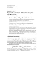
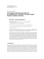
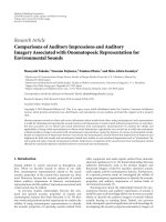
The original S-method, the S-method of reconstructed
signal, as well as the corresponding eigenvalues are shown
in Figure 2. The reconstructed formants that will be used
in watermarking procedure and their support function are
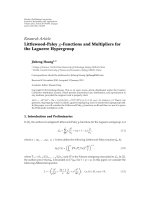
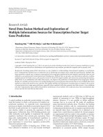
zoomed in Figure 3. The formants separated by the proposed
eigenvalues decomposition are shown in Figure 4 (although
K
= 20 is used, only ten formants are related to the positive
frequency axes).
5. Time-Frequency-Based Speech
Water mar king Pro cedure
5.1. Watermark Modelling and Embedding. The time-
frequency representation of the formants selected from
SM
f
K
rec
(t, ω) is used as a time-frequency mask to shape
the watermark. This time-frequency representation is
6 EURASIP Journal on Advances in Signal Processing
Original signal (SM) Reconstructed formants (SM)
Frequency
Frequency
Time Time
(a)
0 2 4 6 8 10 12 14 16 18 20
0
5

10
15
20
Eigenvalue number
Components eigenvalues
(b)
0 2 4 6 8 10 12 14 16 18 20
0
1
2
3
Eigenvector number
Components concentration (log scale)
(c)
Figure 2: An illustration of the formants reconstruction by using
the eigenvalues decomposition method.
an arbitrary combination of decomposed formants. The pro-
cedure for watermark modelling can be described through
the following steps:
(1) consider a random sequence s,
(2) calculate the STFT of the sequence s denoted as
STFT
s
(t, ω),
(3) the support function L
H
(t, ω) is defined by using
SM
f
K

rec
(t, ω) as follows:
L
H
(
t, ω
)
=
⎧
⎪
⎨
⎪
⎩
1, for



SM
f
K
rec
(
t, ω
)



>λ,
0, otherwise,
(26)

where λ could be set to zero or, for a sharpen mask,
to a small positive value,
(a) (b)
Figure 3: The reconstructed region of formants and the corre-
sponding support function.
(4) finally, the watermark is obtained at the output of the
time-varying filter as follows [19]:
wat
(
t
)
=

ω
L
H
(
t, ω
)
STFT
s
(
t, ω
)
. (27)
The signal is watermarked according to
x
w
(
t

)
=

ω
(
STFT
x
(
t, ω
)
+ L
H
(
t, ω
)
STFT
s
(
t, ω
))
, (28)
where STFT
x
(t, ω) is the STFT of the host signal within the
selected region.
5.2. Watermark Detection. Following the similar concept
as in the embedding process, the watermark detection is
performed, within the time-frequency domain, by using the
standard correlation detector [19]
Det

(
wat
)
=

t

ω
SM
x
w
(
t, ω
)
SM
wat
(
t, ω
)
, (29)
where SM
x
w
(t, ω)andSM
wat
(t, ω) are the S-method of the
watermarked signal and watermark, respectively.
The watermark detection is tested by using a set of wrong
keys (trials), created in the same way as the watermark.
Hence, the successful detection is provided if

Det
(
wat
)
> Det

wrong

, (30)
that is, if

t

ω
SM
x
w
(
t, ω
)
SM
wat
(
t, ω
)
>

t

ω

SM
x
w
(
t, ω
)
SM
wrong
(
t, ω
)
(31)
holds for any wrong trial.
EURASIP Journal on Advances in Signal Processing 7
50
100
150
200
250
200 600 1200
50
100
150
200
250
200 600 1200
50
100
150
200

250
200 600 1200
50
100
150
200
250
200 600 1200
50
100
150
200
250
200 600 1200
50
100
150
200
250
200 600 1200
50
100
150
200
250
200 600 1200
50
100
150
200

250
200 600 1200
50
100
150
200
250
200 600 1200
50
100
150
200
250
200 600 1200
Figure 4: The formants components isolated by using the eigenvalues decomposition method.
Note that the S-method is used in the detection pro-
cedure. The detection performance is improved due to the
higher components concentration. Additionally, for larger
values of L (in the S-method), the cross-terms appear
and they are included in detection, as well [19]. Namely,
the cross-terms also contain the watermark, and hence
they contribute to the watermark detection. The detection
performance is tested by using the following measure of
detection quality [24, 25]:
R
=
D
w
r
− D

w
w

σ
2
w
r
+ σ
2
w
w
, (32)
where
D and σ
2
represent the mean value and the standard
deviation of the detector responses, while the subscripts w
r
and w
w
indicate the right and wrong keys (trials), respec-
tively. The corresponding probability of error is calculated as
follows:
Perr
=
1
4
erfc

R

2

−
1
4
erfc

−
R
2

+
1
2
. (33)
6. Examples
Example 1. In this example, we will demonstrate the advan-
tages of the proposed formants selection procedure over the
threshold-based procedure given in [19]. Namely, two cases
are observed.
(1) Formants whose energy is above a threshold ξ are
selected for watermarking. The threshold is deter-
mined as a portion of the S-method’s maximum
value ξ
= λ10
λlog
10
(max |SM|)
(max |SM|is the max-
imum energy value of the S-method within the

observed region), [19]. Thus, the threshold is adapted
to the maximum energy within the region.
(2) The eigenvalues-based decomposition is used to
create an arbitrary composed time-frequency map.
In the first case, the number of selected formants depends
on the threshold value. An illustration of formants selected
by using two different thresholds ξ
1
and ξ
2
(ξ
1
>ξ
2
)isgiven
in Figure 5(a). Note that a higher threshold ξ
1
(calculated for
λ
1
= 0.85) selects only the strongest low-frequency formants
(Figure 5(a) left). On the other hand, a lower threshold ξ
2
(for λ
2
= 0.3) yields more components (Figure 5(a) right).
However, it is difficult to control their number. Also, the
amount of signal energy is varying through different time-
frequency regions. Thus, an optimal threshold should be
determined for each region. This is a demanding task and

it could cause difficulties in practical applications. Namely, if
the threshold selects too many components, the watermark
may produce perceptual changes. Otherwise, if there are
8 EURASIP Journal on Advances in Signal Processing
(a)
(b)
Figure 5: (a) The components selected by two different thresholds
ξ
1
and ξ
2
(ξ
1
>ξ
2
) within the same region. (b) The components
selected within two different regions when the threshold is 0.6
·
10
0.6log
10
(max |SM|)
.
not enough components, it could be difficult to detect the
watermark. An illustration of two different regions, obtained
by using the threshold ξ with λ
= 0.6, is given in Figure 5(b).
Although the threshold is calculated for both regions in
the same way 0.6
· 10

0.6log
10
(max |SM|)
, the number of selected
components is significantly different. The components in
the first region (Figure 5(b)left) are approximately at the
same energy level. Thus, a significant number of them will
be selected with this threshold. However, in the second
region (Figure 5(b) right), the energy varies for different
components and the given threshold selects just a few
strongest components.
On the other hand, the eigenvalues decomposition
method provides a flexible choice of the components
number. Furthermore, it is possible to arbitrarily com-
bine the components that belong to the low-, middle- or
high-frequency regions. Consequently, an arbitrary time-
frequency mask can be composed as a combination of signal
components. It will be used for watermark modelling. Some
illustrative examples are shown in Figure 6. Each component
is available separately and we can freely choose the number
and positions of the components that we intend to use within
the time-frequency mask. For instance, when observing
the region in Figure 5(a) (right), we can combine a few
strong low-frequency components with a few high-frequency
Figure 6: Illustrations of components selections provided by the
proposed method.
components, as shown in Figure 6 (upper row, left), which
could be difficult to achieve by using the threshold-based
approach.
Example 2. The speech signal with maximal frequency 4 kHz

is considered. A voiced time-frequency region is used for
watermark modelling and embedding. The procedure is
implemented in Matlab 7. The STFT is calculated using the
rectangular window with 1024 samples, and then, it is used
to obtain the signal S-method. Since the speech components
are very close to each other in the time-frequency domain,
the S-method is calculated with the parameter L
= 3toavoid
the presence of cross-terms. After calculating the inverse
transform (the IFFT routine is applied to the S-method),
the eigenvalues and eigenvectors are obtained by using the
Matlab built-in function (eigs). Twenty eigenvectors are
selected, weighted by the corresponding eigenvalues, and
merged into a signal with desired components. Furthermore,
the S-method is calculated for the obtained signal providing
the support function L
H
for watermark shaping. Here, the
Hanning window with 512 samples is used for the STFT
calculation while in the S-method L
= 3. The watermark
is created as a pseudorandom sequence, whose length is
determined by the length of the voiced speech region
(approximately 1300 samples). The STFT of the watermark
is also calculated by using the Hanning window with 512
samples. It is then multiplied by the function L
H
to shape
its time-frequency characteristics. For each of the right keys
(watermarks), a set of 50 wrong trials is created following

the same modelling procedure as for the right keys. The
correlation detector based on the S-method coefficients is
applied with L
= 32.
The proposed approach preserves favourable properties
of the time-frequency-based watermarking procedure [19],
which outperforms some existing techniques. An illustration
EURASIP Journal on Advances in Signal Processing 9
0 500 1000
0
0.5
1
Right keys
Wrong trials
Figure 7: The normalized detector responses for a set of right keys
and wrong trials (for the proposed approach).
of normalized detector responses for right keys (red line) and
wrong trials (blue line) is shown in Figure 7. Furthermore,
the robustness is tested against several types of attacks, all
being commonly used in existing procedures [5, 8, 10].
Namely, in the existing algorithms, the usual amount of
attacks is time scaling up to 4%, wow up to 0.5% or 0.7%,
echo 50 ms or 100 ms [5], and so forth, providing the
probability of error of order 10
−6
. We have applied the same
types of attacks, but with higher strength, showing that the
proposed approach provides robustness even in this case.
The proposed procedure is tested on: mp3 compression with
constant bit rate (128 Kbps), mp3 compression with variable

bit rate (40
−50 Kbps), delay (180 ms), Echo (200 ms), pitch
scaling (5%), wow (delay 20%), flutter, and amplitude
normalization. The measures of detection quality and cor-
responding probabilities of error are calculated according to
(32). The results are given in Tab le 2. Note that the proposed
method provides very low probabilities of error, mostly of
order 10
−7
, even in the presence of stronger attacks. Also,
the robustness to pitch scaling has been improved when
compared to the results reported in [19].
As expected, the detection results are similar as in [19]
where the threshold is well adapted to the energy within the
considered speech region. However, in the previous example,
it is shown that the optimal threshold selection for one
region does not have to be optimal for the other ones.
Thus, it can include only a few formants (Figure 5(b) right).
Consequently, the detection performance decreases, due to
the smaller number of components available for correlation
in the time-frequency domain. The procedure performance
can vary significantly for different regions, since it is not
easy to adjust thresholds separately for each of them. In this
example, a single threshold is used. The detection results
obtained for the region where the threshold is not optimal are
shown in Figure 8. The measures of detection quality have
decreased, as shown in Ta b le 3. From this point of view, the
flexibility of components selection provided by the proposed
approach assures more reliable results.
0 500 1000

0
0.5
1
Right keys
Wrong trials
Figure 8: The normalized detector responses for a set of right keys
and wrong trials; the threshold is not optimal for the considered
region.
Table 2: The measures of detection quality for the proposed
approach under various attacks.
Attack R Perr
No attack 8 10
−9
Mp3 constant 7.2 10
−7
Mp3 variable 6.8 10
−7
Delay 7 10
−7
Echo 6.9 10
−7
Pitch scaling 6.4 10
−6
Wow 6. 2 10
−6
Bright flutter 6.8 10
−7
Amplitude normalization 6.2 10
−6
Table 3: The measures of detection quality.

Attack R
No attack 4.3
Mp3 constant 4.1
Mp3 variable 3.9
Delay 4
Echo 4
Pitch scaling 3.9
Wow 1. 8
Bright flutter 3.8
Amplitude normalization 4.1
The proposed procedure is secure in the following sense:
the watermark is shaped and added directly to the formants
in the time-frequency domain, and thus, it is hard to
remove it without the key, which is assumed to be private
(hidden). Namely, supposing that the quality of voiced data
is important for the application, any attempt to remove the
watermark will produce significant quality degradation. In
order to achieve higher degree of security, the watermarking
can be combined with the cryptography [26]. For example,
10 EURASIP Journal on Advances in Signal Processing
the cryptography can be used to prove the presence of a
specific watermark in a digital object without compromising
the watermark security.
7. Conclusion
The paper proposes an improved formants selection method
for speech watermarking purposes. Namely, the eigenvalues
decomposition based on the S-method is used to select
different formants within the time-frequency regions of
speech signal. Unlike the threshold-based selection, the pro-
posed method allows for an arbitrary choice of components

number and their positions in the time-frequency plane.
This method results in better performance when compared
to the method based on a single threshold. An additional
improvement is achieved by adapting the Hermite projection
method for characterization of speech regions. This has led
to an efficient selection of voiced regions with formants
suitable for watermarking. Finally, the watermarking pro-
cedure based on the proposed approach provides greater
flexibility in implementation and it is characterised by
reliable detection results.
Acknowledgment
This work is supported by the Ministry of Education and
Science of Montenegro.
References
[1] S. K. Pal, P. K. Saxena, and S. K. Mutto, “The future of audio
steganography,” in Proceedings of Pacific Rim Workshop on
Digital Steganography, 2002.
[2] N. Cvejic and T. Sepp
¨
anen, “Increasing the capacity of LSB
based audio steganography,” in Proceedings of the 5th IEEE
International Workshop on Multimedia Signal Processing,pp.
336–338, St. Thomas, Virgin Islands, USA, December 2002.
[3] C S. Shieh, H C. Huang, F H. Wang, and J S. Pan, “Genetic
watermarking based on transform-domain techniques,” Pat-
tern Recognition, vol. 37, no. 3, pp. 555–565, 2004.
[4] F H. Wang, L. C. Jain, and J S. Pan, “VQ-based watermarking
scheme with genetic codebook partition,” Journal of Network
and Computer Applications, vol. 30, no. 1, pp. 4–23, 2007.
[5] D. Kirovski and H. S. Malvar, “Spread-spectrum watermarking

of audio signals,” IEEE Transactions on Signal Processing, vol.
51, no. 4, pp. 1020–1033, 2003.
[6] H. Malik, R. Ansari, and A. Khokhar, “Robust audio water-
marking using frequency-selective spread spectrum,” IET
Information Security, vol. 2, no. 4, pp. 129–150, 2008.
[7] N. Cvejic, A. Keskinarkaus, and T. Seppanen, “Audio water-
marking using m-sequences and temporal masking,” in Pro-
ceedings of IEEE Workshop on Applications of Signal Processing
to Audio and Acoustics, pp. 227–230, New York, NY, USA,
October 2001.
[8] N. Cvejic, Algorithms for audio watermarking and steganogra-
phy, Academic dissertation, University of Oulu, Oulu, Finland,
2004.
[9] S S. Kuo, J. D. Johnston, W. Turin, and S. R. Quackenbush,
“Covert audio watermarking using perceptually tuned signal
independent multiband phase modulation,” in Proceedings of
IEEE International Conference on Acoustic, Speech and Signal
Processing, pp. 1753–1756, Orlando, Fla, USA, May 2002.
[10] S. Xiang and J. Huang, “Histogram-based audio watermarking
against time-scale modification and cropping attacks,” IEEE
Transactions on Multimedia, vol. 9, no. 7, pp. 1357–1372, 2007.
[11] K. Hofbauer, H. Hering, and G. Kubin, “Speech watermarking
for the VHF radio channel,” in Proceedings of EUROCON-
TROL Innovative Research Workshop (INO ’05), pp. 215–220,
Br
´
etigny-sur-Orge, France, December 2005.
[12] L. Cohen, “Time-frequency distributions—a review,” Proceed-
ings of the IEEE, vol. 77, no. 7, pp. 941–981, 1989.
[13] P. J. Loughlin, “Scanning the special issue on time-frequency

analysis,” Proceedings of the IEEE, vol. 84, no. 9, p. 1195, 1996.
[14] B. Boashash, Time-Frequency Analysis and Processing,Elsevier,
Amsterdam, The Netherlands, 2003.
[15] F. Hlawatsch and G. F. Boudreaux-Bartels, “Linear and
quadratic time-frequency signal representations,” IEEE Sign al
Processing Magazine, vol. 9, no. 2, pp. 21–67, 1992.
[16] L. Stankovic, “Method for time-frequency analysis,” IEEE
Transactions on Signal Processing, vol. 42, no. 1, pp. 225–229,
1994.
[17] L. Stankovi
´
c, T. Thayaparan, and M. Dakovi
´
c, “Signal decom-
position by using the S-method with application to the
analysis of HF radar signals in sea-clutter,” IEEE Transactions
on Signal Processing, vol. 54, no. 11, pp. 4332–4342, 2006.
[18] T. Thayaparan, L. Stankovi
´
c, and M. Dakovi
´
c, “Decompo-
sition of time-varying multicomponent signals using time-
frequency based method,” in Proceedings of Canadian Confer-
ence on Electrical and Computer Engineering (CCECE ’06),pp.
60–63, Ottawa, Canada, May 2006.
[19] S. Stankovi
´
c, I. Orovi
´

c, and N.
ˇ
Zari
´
c, “Robust speech water-
marking procedure in the time-frequency domain,” EURASIP
Journal on Advances in Signal Processing, vol. 2008, Article ID
519206, 9 pages, 2008.
[20] S. Stankovi
´
c, I. Orovi
´
c, N.
ˇ
Zari
´
c,andC.Ioana,“Anapproach
to digital watermarking of speech signals in the time-
frequency domain,” in Proceedings of the 48th International
Symposium focused on Multimedia Signal Processing and
Communications (ELMAR ’06), pp. 127–130, Zadar, Croatia,
June 2006.
[21] D. Kortchagine and A. Krylov, “Image database retrieval by
fast Hermite projection method,” in Proceedings of the 15th
International Conference on Computer Graphics and Applica-
tions (GraphiCon ’05), pp. 308–311, Novosibirsk Akadem-
gorodok, Russia, June 2005.
[22] D. Kortchagine and A. Krylov, “Projection filtering in image
processing,” in Proceedings of the 10th International Conference
on Computer Graphics and Applications (GraphiCon ’00),pp.

42–45, Moscow, Russia, August-September 2000.
[23] S. Stankovi
´
c, “About time-variant filtering of speech signals
with time-frequency distributions for hands-free telephone
systems,” Signal Processing, vol. 80, no. 9, pp. 1777–1785, 2000.
[24] D. Heeger, Signal Detection Theory,DepartmentofPsychiatry,
Stanford University, Stanford, Calif, USA, 1997.
[25] T. D. Wickens, Elementary Signal Detection Theory,Oxford
University Press, Oxford, UK, 2002.
[26] A. Adelsbach, S. Katzenbeisser, and A R. Sadeghi, “Water-
mark detection with zero-knowledge disclosure,” Multimedia
Systems, vol. 9, no. 3, pp. 266–278, 2003.