Báo cáo hóa học: " Research Article High-Quality Time Stretch and Pitch Shift Effects for Speech and Audio Using the Instantaneous Harmonic Analysis" pdf

Hindawi Publishing Corporation
EURASIP Journal on Advances in Signal Processing
Volume 2010, Article ID 712749, 10 pages
doi:10.1155/2010/712749
Research Article
High-Quality Time Stretch and Pitch Shift Effects for Speech and
Audio Using the Instantaneous Harmonic Analysis
Elias Azarov,
1
Alexander Petrovsky (EURASIP Member),
1, 2
and Marek Parfieniuk (EURASIP Member)
2
1
Department of Computer Engineering, Belarussian State University of Informatics and Radioelectronics, 220050 Minsk, Belarus
2
Department of Real-Time Systems, 15-351 Bialystok University of Technology, Bialystok, Poland
Correspondence should be addressed to Alexander Petrovsky,
Received 6 May 2010; Accepted 10 November 2010
Academic Editor: Udo Zoelzer
Copyright © 2010 Elias Azarov et al. This is an open access article distributed under the Creative Commons Attribution License,
which permits unrestricted use, distribution, and reproduction in any medium, provided the original work is properly cited.
The paper presents methods for instantaneous harmonic analysis with application to high-quality pitch, timbre, and time-scale
modifications. The analysis technique is based on narrow-band filtering using special analysis filters with frequency-modulated
impulse response. The main advantages of the technique are high accuracy of harmonic parameters estimation and adequate
harmonic/noise separation that allow implementing audio and speech effects with low level of audible artifacts. Time stretch and
pitch shift effects are considered as primary application in the paper.
1. Introduction
Parametric representation of audio and speech signals has
become integral part of moder n effect technologies. The
choice of an appropriate parametric model significantly

defines overall quality of implemented effects. The present
paper describes an approach to parametric signal processing
based on deterministic/stochastic decomposition. The signal
is considered as a sum of periodic (harmonic) and residual
(noise) parts. The p eriodic part can be efficiently described
as a sum of sinusoids with slowly varying amplitudes and
frequencies, and the residual part is assumed to be irregular
noise signal. This representation was introduced in [1]and
since then has been profoundly studied and significantly
enhanced. The model provides good parameterization of
both voiced and unvoiced frames and allows using different
modification techniques for them. It insures effective and
simple processing in frequency domain; however, the crucial
point there is accuracy of harmonic analysis. The harmonic
part of the signal is specified by sets of harmonic parameters
(amplitude, frequency, and phase) for every instant of time.
A number of methods have been proposed to estimate
these parameters. The majority of analysis methods assume
local stationarity of amplitude and frequency parameters
within the analysis frame [2, 3]. It makes the analysis
procedure easier but, on the other hand, degrades parameters
estimation and periodic/residual separation accuracy.
Some good alternatives are methods that make esti-
mation of instantaneous harmonic parameters. The notion
of instantaneous frequency was introduced in [4, 5], the
estimation methods have been presented in [4–9]. The aim
of the current investigation is to study applicability of the
instantaneous harmonic analysis technique described in [8,
9] to a processing system for making audio and speech effects
(such as pitch, timbre, and time-scale modifications). The

analysis method is based on narrow-band filtering using
analysis filters with closed form impulse response. It has been
shown [8] that analysis filters can be adjusted in accordance
with pitch contour in order to get adequate estimate of
high-order harmonics with rapid frequency modulations.
The technique presented in this paper has the following
improvements:
(i) simplified closed form expressions for instantaneous
parameters estimation;
(ii) pitch detection and smooth pitch contour estimation;
(iii) improved har monic parameters estimation accuracy.
The analysed signal is separated into periodic and
residual parts and then processed through modification tech-
niques. Then the processed signal can be easily synthesized
2 EURASIP Journal on Advances in Signal Processing
in time domain at the output of the system. The deter-
ministic/stochastic representation significantly simplifies the
processing stage. As it is shown in the experimental section,
the combination of the proposed analysis, processing, and
synthesis techniques provides good quality of signal analysis,
modification, and reconstruction.
2. Time-Frequency Representations and
Harmonic Analysis
The sinusoidal model assumes that the signal s(n)canbe
expressed as the sum of its periodic and stochastic parts:
s
(
n
)
=

K

k=1
MAG
k
(
n
)
cos ϕ
k
(
n
)
+ r
(
n
)
,(1)
where MAG
k
(n)—the instantaneous magnitude of the kth
sinusoidal component, K is the number of components,
ϕ
k
(n) is the instantaneous phase of the kth component,
and r(n) is the stochastic part of the signal. Instantaneous
phase ϕ
k
(n) and instantaneous frequency f
k

(n) are related as
follows:
ϕ
k
(
n
)
=
n

i=0
2πf
k
(
i
)
F
s
+ ϕ
k
(
0
)
,(2)
where F
s
is the sampling frequency and ϕ
k
(0) is the initial
phase of the kth component. The harmonic model states that

frequencies f
k
(n) are integer multiples of the fundamental
frequency f
0
(n) and can be calculated as
f
k
(
n
)
= kf
0
(
n
)
. (3)
The harmonic model is often used in speech coding since
it represents voiced speech in a highly efficient way. The
parameters MAG
k
(n), f
k
(n), and ϕ
k
(0) are estimated by
means of the sinusoidal (harmonic) analysis. The stochastic
part obviously can be calculated as the difference between the
source signal and estimated sinusoidal part:
r

(
n
)
= s
(
n
)
−
K

k=1
MAG
k
(
n
)
cos ϕ
k
(
n
)
. (4)
Assuming that sinusoidal components are stationary (i.e.,
have constant amplitude and frequency) over a short period
of time that correspond to the length of the analysis frame,
they can be estimated using DFT:
S

f


=
1
N
N−1

n=0
s
(
n
)
e
− j2πnf/N
,(5)
where N is the length of the frame. The transformation
gives spectral representation of the signal by sinusoidal
components of multiple frequencies. The balance between
frequency and time resolution is defined by the length of the
analysis frame N. Because of the local stationarity assump-
tion DFT can hardly provide accurate estimate of frequency-
modulated components that gives rise to such approaches
as harmonic transform [10] and fan-chirp transform [11].
The general idea of these approaches is using the Fourier
transform of the warped-time signal.
The signal warping can be carried out before transforma-
tion or directly embedded in the transform expression [11]:
S
(
ω, α
)
=

∞

n=−∞
s
(
n
)

|1+αn|e
− jω(1+(1/2)αn)n
,(6)
where ω is frequency a nd α is the chirp rate. The trans-
form is able to identify components with linear frequency
change; however, their spectral amplitudes are assumed
to be constant. There are several methods for estimation
instantaneous harmonic parameters. Some of them are
connected with the notion of analytic signal based on the
Hilbert transform (HT). A unique complex signal z(t)from
arealones(t) can be generated using the Fourier transform
[12]. This also can be done as the following time-domain
procedure:
z
(
t
)
= s
(
t
)
+ jH

[
s
(
t
)
]
= a
(
t
)
e
jϕ(t)
,(7)
where H is the Hilbert transform, defined as
H
[
s
(
t
)
]
= p.v.

+∞
−∞
s
(
t − τ
)
πτ

dτ,(8)
where p.v. denotes Cauchy principle value of the integral.
z(t) is referred to as Gabor’s complex signal, and a(t)and
ϕ(t) can be considered as the instantaneous amplitude and
instantaneous phase, respectively. Signals s(t)andH[s(t)] are
theoretically in quadrature. Being a complex signal z(t)can
be expressed in polar coordinates, and therefore a(t)andϕ(t)
can be calculated as follows:
a
(
t
)
=

s
2
(
t
)
+ H
2
[
s
(
t
)
]
,
ϕ
(

t
)
= arc tan

H
[
s
(
t
)
]
s
(
t
)

.
(9)
Recently the discrete energy s eparation algorithm (DESA)
based on the Teager energy operator was presented [5]. The
energy operator is defined as
Ψ
[
s
(
n
)
]
= s
2

(
n
)
− s
(
n − 1
)
s
(
n +1
)
, (10)
where the derivative operation is approximated by the
symmetric difference. The instantaneous amplitude MAG(n)
and frequency f (n) can be evaluated as
MAG
(
n
)
=
2Ψ
[
s
(
n
)
]

Ψ
[

s
(
n +1
)
− s
(
n − 1
)
]
,
f
(
n
)
= arc sin

Ψ
[
s
(
n +1
)
− s
(
n − 1
)
]
4Ψ
[
s

(
n
)
]
.
(11)
The Hilbert transform and DESA can be applied only to
monocomponent signals as long as for multicomponent
signals the notion of a single-valued instantaneous frequency
and amplitude becomes meaningless. Therefore, the signal
should be split into single components before using these
techniques. It is possible to use nar row-band filtering for this
purpose [6]. However, in the case of frequency-modulated
components, it is not always possible due to their wide
frequency.
EURASIP Journal on Advances in Signal Processing 3
3. Instantaneous Harmonic Analysis
3.1. Instantaneous Harmonic Analysis of Nonstationary Har-
monic Components. The proposed analysis method is based
on the filtering technique that provides direct parameters
estimation [8]. In voiced speech harmonic components
are spaced in frequency domain and each component can
be limited thereby a narrow frequency band. Therefore
harmonic components can be separated within the analysis
frame by filters with nonoverlapping bandwidths. These
considerations point to the applicability and effectiveness
of the filtering approach to harmonic analysis. The signal
s(n) is represented as a sum of bandlimited cosine functions
with instantaneous amplitude, phase, and frequency. It is
assumed that harmonic components are spaced in frequency

domain so that each component can be limited by a narrow
frequency band. The harmonic components can be separated
within the analysis frame by filters with nonoverlapping
bandwidths. Let us denote the number of cosines L and
frequency separation borders (in Hz) F
0
≤ F
2
≤ ··· ≤ F
L
,
where F
0
= 0, F
L
= F
s
/2. The given signal s(n)canbe
represented as its convolution with the impulse response of
the ideal low-pass filter h(n):
s
(
n
)
= s
(
n
)
∗ h
(

n
)
= s
(
n
)
∗
sin
(
πn
)
nπ
= s
(
n
)
∗

0.5
−0.5
cos

2πfn

df
= s
(
n
)
∗


2

0.5
0
cos

2πfn

df

=
s
(
n
)
∗
⎡
⎣
L

k=1
2
F
s

F
k
F
k−1

cos

2πf
n
F
s

df
⎤
⎦
=
L

k=1
s
(
n
)
∗

2
F
s
h
k
(
n
)

=

L

k=1
s
k
(
n
)
,
(12)
where h
k
(n)—the impulse response of the band-pass filter
with passband [F
k−1
, F
k
], s
k
(n)—bandlimited output signal.
The impulse response can be written in the following way:
h
k
(
n
)
=

F
k

F
k−1
cos

2πf
n
F
s

df
=
⎧
⎪
⎪
⎨
⎪
⎪
⎩
2F
k
Δ
, n = 0,
F
s
nπ
cos

2πn
F
s

F
k
c

sin

2πn
F
s
F
k
Δ

, n
/
= 0,
(13)
where F
k
c
= (F
k−1
+F
k
)/2andF
k
Δ
= (F
k
−F

k−1
)/2. Parameters
F
k
c
and F
k
Δ
correspond to the center frequency of the passband
and the half of bandwidth, respectively. Convolution of finite
signal s(n)(0
≤ n ≤ N − 1) and h
k
(n) can be expressed as the
following sum:
s
k
(
n
)
=
N−1

i=0
2s
(
i
)
π
(

n − i
)
cos

2π
(
n − i
)
F
s
F
k
c

sin

2π
(
n − i
)
F
s
F
k
Δ

.
(14)
The expression can be rewritten as a sum of zero frequency
components:

s
k
(
n
)
= A
(
n
)
cos
(
0n
)
+ B
(
n
)
sin
(
0n
)
, (15)
where
A
(
n
)
=
N−1


i=0
2s
(
i
)
π
(
n − i
)
sin

2π
(
n − i
)
F
s
F
k
Δ

cos

2π
(
n − i
)
F
s
F

k
c

,
B
(
n
)
=
N−1

i=0
−2s
(
i
)
π
(
n − i
)
sin

2π
(
n − i
)
F
s
F
k

Δ

sin

2π
(
n − i
)
F
s
F
k
c

.
(16)
Thus, considering (15), the expression (14) is a magnitude
and frequency-modulated cosine function:
s
k
(
n
)
= MAG
(
n
)
cos

ϕ

(
n
)

, (17)
with instantaneous magnitude MAG(n), phase ϕ(n), and
frequency f (n) that can be calculated as
MAG
(
n
)
=

A
2
(
n
)
+ B
2
(
n
)
,
ϕ
(
n
)
= arc tan


−
B
(
n
)
A
(
n
)

,
f
(
n
)
=
ϕ
(
n +1
)
− ϕ
(
n
)
2π
F
s
.
(18)
In that way the signal frame s(n)(0

≤ n ≤ N − 1) can
be represented by L cosines with instantaneous amplitude
and frequency. Instantaneous sinusoidal parameters of the
filter output are available at every instant of time within the
analysis frame. The filter output s
k
(n) can be interpreted as
an analytical signal s
a
k
(n) in the following way :
s
a
k
(
n
)
= A
(
n
)
+ jB
(
n
)
. (19)
The bandwidth specified by border frequencies F
k−1
and F
k

(or by parameters F
k
c
and F
k
Δ
) should cover the frequency
of the periodic component that is being analyzed. In many
applications there is no need to represent entire signal as
a sum of modulated cosines. In hybrid parametric repre-
sentation it is necessary to choose harmonic components
with smooth contours of frequency and amplitude values.
For accurate sinusoidal parameters estimation of periodical
components with high-frequency modulations a frequency-
modulated filter can be used. The closed form impulse
response of the filter is modulated according to frequency
contour of the analyzed component. This approach is
quite applicable to analysis of voiced speech since rough
harmonic frequency trajectories can be estimated from the
pitch contour. Considering centre frequency of the filter
bandwidth as a function of time F
c
(n), (15)canberewritten
in the following form:
s
k
(
n
)
= A

(
n
)
cos
(
0n
)
+ B
(
n
)
sin
(
0n
)
, (20)
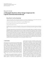
4 EURASIP Journal on Advances in Signal Processing
650
600
550
500
450
400
1000 200 300 400 500
Samples
Frequency (Hz)
F(n)
F
c
(n)

F
c
(n) ± F
Δ
F
Δ
Figure 1: Frequency-modulated analysis filter N = 512.
where
A
(
n
)
=
N−1

i=0
2s
(
i
)
π
(
n − i
)
sin

2π
(
n − i
)

F
s
F
k
Δ

cos

2π
F
s
ϕ
c
(
n, i
)

,
B
(
n
)
=
N−1

i=0
−2s
(
i
)

π
(
n − i
)
sin

2π
(
n − i
)
F
s
F
k
Δ

sin

2π
F
s
ϕ
c
(
n, i
)

,
ϕ
c

(
n, i
)
=
⎧
⎪
⎪
⎪
⎪
⎪
⎪
⎪
⎪
⎨
⎪
⎪
⎪
⎪
⎪
⎪
⎪
⎪
⎩
i

j=n
F
k
c


j

, n<i,
−
n

j=i
F
k
c

j

, n>i,
0, n
= i.
(21)
The required instantaneous parameters can be calculated
using expressions (18). The frequency-modulated filter has
a warped band pass, aligned to the given frequency contour
F
k
c
(n) that provides adequate analysis of periodic compo-
nents with rapid frequency alterations. This approach is an
alternative to time warping that is used in speech analysis
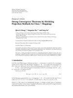
[11]. In Figure 1 an example of parameters estimation is
shown. The frequency contour of the harmonic component
can be covered by the filter band pass specified by the centre
frequency contour F

k
c
(n) and the bandwidth 2F
k
Δ
.
Center frequency contour F
c
(n) is adjusted within the
analysis frame providing narrow-band filtering of frequency-
modulated components.
3.2. Filter Properties. Estimation accuracy degrades close
to borders of the frame because of signal discontinuity
and spectral leakage. However, the estimation error can be
reduced using wider passband—Figure 2.
In any case the passband should be wide enough in order
to provide adequate estimation of harmonic amplitudes. If
the passband is too narrow, the evaluated amplitude values
become lower than they are in reality. It is possible to
1000 200 300 400 500
Samples
Actual values
Estimated values
Estimated values
0
0.2
0.4
0.6
0.8
1

Amplitude
(wide-band filtering)
(narrow band filtering)
Figure 2: Instantaneous amplitude estimation accuracy.
450
360
275
160
90
0
0 0.03 0.065 0.095 0.125 0.16
Time (s)
Bandwidth (Hz)
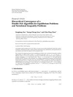
Figure 3: Minimal bandwidth of analysis filter.
determine the filter bandwidth as a threshold value that gives
desired level of accuracy. The threshold value depends on
length of analysis window and type of window function. In
Figure 3 the dependence for Hamming window is presented,
assuming that amplitude attenuation should be less than
−20 dB.
It is evident that required bandwidth becomes more
narrow when the length of the window increases. It is also
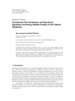
clear that a wide passband affects estimation accuracy when
the signal contains noise. The noise sensitivity of the filters
with different bandwidths is demonstrated in Figure 4.
3.3. Estimation Technique. In this subsection the general
technique of sinusoidal parameters estimation is presented.
The technique does not assume harmonic structure of the
signal and therefore can be applied both to speech and audio
signals [13].

In order to locate sinusoidal components in frequency
domain, the estimation procedure uses iterative adjustments
of the filter bands with a predefined number of iterations—
Figure 5. At every step the centre frequency of each filter is
changed in accordance with the calculated frequency value
in order to position energy peak at the centre of the band. At
EURASIP Journal on Advances in Signal Processing 5
Time (s)
10 Hz bandwidth
50 Hz bandwidth
90 Hz bandwidth
4
3.2
2.45
1.6
0.75
0
Mean error (Hz)
−10 −50 5 1015
Figure 4: Instantaneous frequency estimation error.
the initial stage, the frequency range of the signal is covered
by overlapping bands B
1
, , B
h
(where h is the number of
bands) with constant central frequencies F
B
1
C

, , F
B
h
C
,respec-
tively. At every step the respective instantaneous frequencies
f
B
1
(n
c
), , f
B
h
(n
c
)areestimatedbyformulas(15)and(18)
at the instant that corresponds to the centre of the frame
n
c
. Then the central bandwidth frequencies are reset F
B
x
C
=
f
B
x
(n
c

), and the next estimation is carried out. When all
the energy peaks are located, the final sinusoidal parameters
(amplitude, frequency, and phase) can be calculated using
the expressions (15)and(18) as well. During the peak
location process, some of the filter bands may locate the
same component. Duplicated parameters are discarded by
comparison of the centre band frequencies F
B
1
C
, , F
B
h
C
.
In order to discard short-term components (that appar-
ently are transients or noise and should be taken to the resid-
ual), sinusoidal par ameters are tracked from frame to frame.
The frequency and amplitude values of adjacent frames are
compared, providing long-term component matching. The
technique has been used in the hybrid audio coder [13],
since it is able to pick out the sinusoidal part and leave the
original transients in the residual without any prior transient
detection. In Figure 6 a result of the signal separation is
presented. The source signal is a jazz tune (Figure 6(a)).
The analysis was carried out using the following set-
tings: analysis frame length—48 ms, analysis step—14 ms,
filter bandwidths—70 Hz, and windowing function—the
Hamming window. The synthesized periodic part is shown
in Figure 6(b). As can be seen from the spectrogram, the

periodic part contains only long sinusoidal components with
high-energy localization. The transients are left untouched in
the residual signal that is presented in Figure 6(c).
3.4. Speech Analysis. In speech processing, it is assumed
that signal frames can be either voiced or unvoiced. In
voiced segments the periodical constituent prevails over
the noise, in unvoiced segments the opposite takes place,
and therefore any harmonic analysis is unsuitable in that
case. In the proposed analysis framework voiced/unvoiced
frame classification is carried out using pitch detector. The
harmonic parameters estimation procedure consists of the
two following stages:
(i) initial fundamental frequency contour estimation;
(ii) harmonic parameters estimation with fundamental
frequency adjustment.
In voiced speech analysis, the problem of initial fun-
damental frequency estimation comes to finding a peri-
odical component with the lowest possible frequency and
sufficiently high energy. Within the possible fundamental
frequency range (in this paper, it is defined as [60, 1000] Hz)
all periodical components are extracted, and then the
suitable one is considered as the fundamental. In order to
reduce computational complexity, the source signal is filtered
by a low-pass filter before the estimation.
Having fundamental contour estimated, it is possible to
calculate filter impulse responses aligned to the fundamental
frequency contour. Central frequency of the filter band is
calculated as the instantaneous frequency of fundamental
multiplied by the number k of the correspondent harmonic
F

k
C
(n) = kf
0
(n). The procedure goes from the first harmonic
to the last, adjusting fundamental frequency at every step—
Figure 7. The fundamental frequency recalculation formula
can be written as follows:
f
0
(
n
)
=
k

i=0
f
i
(
n
)
MAG
i
(
n
)
(
i +1
)


k
j=0
MAG
j
(
n
)
. (22)
The fundamental frequency values become more precise
while moving up the frequency range. It allows making
proper analysis of high-order harmonics with significant
frequency modulations. Harmonic parameters are estimated
using expressions (10)-(11). After parameters estimation, the
periodical par t of the signal is synthesized by formula (1)and
subtracted from the source in order to get the noise part.
In order to test applicability of the proposed technique,
a set of synthetic signals with predefined parameters was
used. The signals were synthesized with different harmonic-
to-noise ratio defined as
HNR
= 10lg
σ
2
H
σ
2
e
, (23)
where σ

2
H
is the energy of the deterministic part of the signal
and σ
2
e
is the energy of its stochastic part. All the signals were
generated using a specified fundamental frequency contour
f
0
(n) and the same number of harmonics—20. Stochastic
parts of the signals were generated as white noise with such
energy that provides specified HNR values. After analysis the
signals were separated into stochastic and deterministic parts
with new harmonic-to-noise ratios:

HNR = 10lg
σ
2
H
σ
2
e
. (24)
Quantitative characteristics of accuracy were calculated as
signal-to-noise ratio:
SNR
H
= 10lg
σ

2
H
σ
2
eH
, (25)
6 EURASIP Journal on Advances in Signal Processing
B3
−10
0
−20
−30
−40
−50
Amplitude (dB)
35 70
0 105
140
175 210
245 280 315 350 385 420 455
Frequency (Hz)
B6 B9
B12
B10B7B4B1
B2 B5 B8 B11
(a)
−10
0
−20
−30

−40
−50
Amplitude (dB)
65 135165 235 265 335
Frequency (Hz)
B3 B6 B9
(b)
Figure 5: Sinusoidal parameters estimation using analysis filters: (a) initial frequency partition; (b) frequency partition after second iteration.
0
500
1000
1500
2000
2500
3000
3500
4000
Frequency (Hz)
0.5 1 1.5 2 2.5 3
−1
−0.5
0
0.5
1
Time (s)
Amplitude
(a)
0
500
1000

1500
2000
2500
3000
3500
4000
Frequency (Hz)
0.5 1 1.5 2 2.5 3
−1
−0.5
0
0.5
1
Time (s)
Amplitude
(b)
0
500
1000
1500
2000
2500
3000
3500
4000
Frequency (Hz)
0.5 1 1.5 2 2.5 3
−1
−0.5
0

0.5
1
Time (s)
Amplitude
(c)
Figure 6: Periodic/stochastic separation of an audio signal: (a) source signal; (b) periodic part; (c) stochastic part.
EURASIP Journal on Advances in Signal Processing 7
Source speech signal
Downsampling
to 2 kHz
Harmonic
analysis
Best candidate
selection
Pitch contour
recalculation
Harmonic
analysis
Estimated
harmonic
parameters
Figure 7: Harmonic analysis of speech.
where σ
2
H
—energy of the estimated harmonic part and σ
2
eH
—
energy of the estimation error (energy of the difference

between source and estimated harmonic parts). T he signals
were analyzed using the proposed technique and STFT-
based harmonic transform method [10]. During analysis
the same frame length was used (64 ms) and the same
window function (Hamming window). In both methods,
it was assumed that the fundamental frequency contour is
known and that frequency trajectories of the harmonics are
integer multiplies of the fundamental frequency. The results,
reported in Ta ble 1 show that the measured SNR
H
values
decrease with HNR values. However, for nonstationary
signals, the proposed technique provides higher SNR
H
values
even when HNR is low.
An example of natural speech analysis is presented in
Figure 8. The source signal is a phrase uttered by a female
speaker (F
s
= 8 kHz). Estimated harmonic parameters were
used for the synthesis of the signal’s periodic part that was
subtracted from the source in order to get the residual.
All harmonics of the source are modeled by the harmonic
analysis when the residual contains t ransient and noise
components, as can be seen in the respective spectrograms.
4. Effects Implementation
The harmonic analysis described in the prev ious section
results in a set of harmonic parameters and residual signal.
Instantaneous spectral envelopes can be estimated from the

instantaneous harmonic amplitudes and the fundamental
frequency obtained at the analysis stage [14]. The linear
interpolation can be used for this purpose. The set of
frequency envelopes can be considered as a function E(n, f )
of two parameters: sample number and frequency. Pitch
shifting procedure a ffects only the periodic part of the signal
that can be synthesized as follows:
s
(
n
)
=
K

k=1
E

n, f
k
(
n
)

cos ϕ
k
(
n
)
. (26)
Phases of harmonic components

ϕ
k
(n) are calculated accord-
ing to a new fundamental frequency contour
f
0
(n):
ϕ
k
(
n
)
=
n

i=0
2π f
k
(
i
)
F
s
+ ϕ
Δ
k
(
n
)
. (27)

Harmonic frequencies are calculated by formula (3):
f
k
(
n
)
= k f
0
(
n
)
. (28)
Additional phase parameter
ϕ
Δ
k
(n)isusedinordertokeep
the original phases of harmonics relative phase of the
fundamental
ϕ
Δ
k
(
n
)
= ϕ
k
(
n
)

− kϕ
0
(
n
)
. (29)
As long as described pitch shifting does not change spectral
envelope of the source signal and keeps relative phases
of the harmonic components, the processed signal has a
natural sound with completely new intonation. The timbre
of speakers voice is defined by the spectral envelope function
E(n, f ). If we consider the envelope function as a matrix
E
=
⎛
⎜
⎜
⎜
⎜
⎜
⎜
⎝
E
(
0,0
)
··· E

0,
F

s
2

.
.
.
.
.
.
.
.
.
E
(
N,0
)
··· E

N,
F
s
2

⎞
⎟
⎟
⎟
⎟
⎟
⎟

⎠
, (30)
then any timbre modification can be expressed as a con-
version function C(E) that transforms the source envelope
matrix E into a new matrix
E:
E = C
(
E
)
. (31)
Since the periodic part of the signal is expressed by
harmonic parameters, it is easy to synthesize the periodic
part slowing down or stepping up the tempo. Amplitude and
frequency contours should be interpolated in the respective
moments of time, and then the output signal can be
synthesized. The noise part is parameterized by spectral
envelopes and then time-scaled as described in [15]. Separate
periodic/noise processing provides high-quality time-scale
modifications with low level of audible artifacts.
5. Experimental Results
In this section an example of vocal processing is shown. The
concerned processing system is aimed at pitch shifting in
order to assist a singer.
The voice of the singer is analyzed by the proposed
technique and then synthesized with pitch modifications to
assist the singer to be in tune with the accompaniment. The
target pitch contour is predefined by analysis of a reference
8 EURASIP Journal on Advances in Signal Processing
0.2 0.4 0.6 0.8 1 1.2 1.4 1.6 1.8 2

Time (s)
0
500
1000
1500
2000
2500
3000
3500
4000
Frequency (Hz)
−1
−0.5
0
0.5
1
Amplitude
(a)
0.2 0.4 0.6 0.8 1 1.2 1.4 1.6 1.8 2
Time (s)
0
500
1000
1500
2000
2500
3000
3500
4000
Frequency (Hz)

−1
−0.5
0
0.5
1
Amplitude
(b)
0.2 0.4 0.6 0.8 1 1.2 1.4 1.6 1.8 2
Time (s)
0
500
1000
1500
2000
2500
3000
3500
4000
Frequency (Hz)
−1
−0.5
0
0.5
1
Amplitude
(c)
Figure 8: Periodic/stochastic separation of an audio signal: (a) source signal; (b) periodic part; (c) stochastic part.
0
500
1000

1500
2000
2500
3000
3500
4000
Frequency (Hz)
−1
−0.5
0
0.5
1
Time (s)
Amplitude
0.2 0.4 0.6 0.8 1 1.2 1.4 1.6 1.8 2 2.2
Figure 9: Reference signal.
recording. Since only pitch contour is changed, the source
voice maintains its identity. The output signal however is
damped in regions, where the energy of the reference signal
0
500
1000
1500
2000
2500
3000
3500
4000
Frequency (Hz)
−1

−0.5
0
0.5
1
Time (s)
Amplitude
0.2 0.4 0.6 0.8 1 1.2 1.4 1.6 1.8 2 2.2
Figure 10: Source signal.
is low in order to provide proper synchronization with
accompaniment. The reference signal is shown in Figure 9,it
is a recorded male vocal. The recording was made in a studio
EURASIP Journal on Advances in Signal Processing 9
Table 1: Results of synthetic speech analysis.
Harmonic transfor m method Instantaneous harmonic analysis
HNR

HNR SNR
H

HNR SNR
H
Signal 1— f
0
(n) = 150 Hz for all n, random constant harmonic amplitudes
∞ 41.5 41.5 50.4 50.4
40 38.5 41.4 41.2 44.7
20 20.8 29.2 21.9 26.2
10 10.7 19.5 11.9 16.4
0 1.2 9.2 2.9 6.0
Signal 2— f

0
(n) changes from 150 to 220 Hz at a rate of 0.1 Hz/ms, constant harmonic amplitudes that model sound [a]
∞ 41.5 41.5 48.3 48.3
40 38.2 40.7 41.0 44.3
20 21.0 29.5 22.1 26.4
10 11.0 20.3 12 17.1
0 1.3 9.3 2.7 6.5
Signal 3— f
0
(n) changes from 150 to 220 Hz at a rate of 0.1 Hz/ms, variable harmonic amplitudes that model sequence of vowels
∞ 19.6 19.7 34.0 34.0
40 17.3 17.5 31.2 31.8
20 17.7 21.3 20.1 25.5
10 8.7 15.6 10.3 15.1
0
−0.8 7.55 0.94 5.2
Signal 4— f
0
(n) changes from 150 to 220 Hz at a rate of 0.1 Hz/ms, variable harmonic amplitudes that model sequence of vowels, harmonic
frequencies deviate from integer multiplies of f
0
(n)on10Hz
∞ 13.2 14.0 26.9 27.0
40 10.6 11.9 24.8 25.3
20 11.9 13.6 19.3 22.7
10 6.9 12.1 9.6 14
0
−1.6 6.1 0.5 4.2
0
500

1000
1500
2000
2500
3000
3500
4000
Frequency (Hz)
−1
−0.5
0
0.5
1
Time (s)
Amplitude
0.2 0.4 0.6 0.8 1 1.2 1.4 1.6 1.8 2 2.2
Figure 11: Output signal.
with a low level of background noise. The fundamental
frequency contour was estimated from the reference signal
as described in Section 3.AscanbeseenfromFigure 10, the
source vocal has different pitch and is not completely noise
free.
The source signal was analyzed using proposed harmonic
analysis, and then the pitch shifting technique was applied as
has been described above.
The synthesized signal with pitch modifications is shown
in Figure 11. As can be seen the output signal contains the
pitch contour of the reference signal, but still has timbre, and
energy of the source voice. The noise part of the source signal
(including background noise) remained intact.

6. Conclusions
The stochastic/deterministic model can be applied to voice
processing systems. It provides efficient signal parameter-
ization in the way that is quite convenient for making
voice effects such as pitch shifting, timbre and time-scale
modifications. The practical application of the proposed
harmonic analysis technique has shown encouraging results.
The described approach might be a promising solution
10 EURASIP Journal on Advances in Signal Processing
to harmonic parameters estimation in speech and audio
processing systems [13].
Acknowledgment
This work was supported by the Polish Ministry of Science
and Higher Education (MNiSzW) in years 2009–2011 (Grant
no. N N516 388836).
References
[1] T. F. Quatieri and R. J. McAulay, “Speech analysis/synthesis
based on a sinusoidal representation,” IEEE Transactions on
Acoustics, Speech, and Signal Processing,vol.34,no.6,pp.
1449–1464, 1986.
[2] A. S. Spanias, “Speech coding: a tutorial review,” Proceedings of
the IEEE, vol. 82, no. 10, pp. 1541–1582, 1994.
[3] X. Serra, “Musical sound modeling with sinusoids plus noise,”
in Musical Signal Processing, C. Roads, S. Pope, A. Pi-cialli, and
G. De Poli, Eds., pp. 91–122, Swets & Zeitlinger, 1997.
[4] B. Boashash, “Estimating and interpreting the instantaneous
frequency of a signal,” Proceedings of the IEEE,vol.80,no.4,
pp. 520–568, 1992.
[5] P. Maragos, J. F. Kaiser, and T. F. Quatieri, “Energy separation
in signal modulations with application to speech analysis,”

IEEE Transactions on Signal Processing, vol. 41, no. 10, pp.
3024–3051, 1993.
[6] T. Abe, T. Kobayashi, and S. Imai, “Harmonics tracking
and pitch extraction based on instantaneous frequency,” in
Proceedings of the 20th Internat ional Conference on Acoustics,
Speech, and Signal Processing, pp. 756–759, May 1995.
[7] T. Abe and M. Honda, “Sinusoidal model based on instan-
taneous frequency attractors,” IEEE Transactions on Audio,
Speech and Language Processing, vol. 14, no. 4, pp. 1292–1300,
2006.
[8] E. Azarov, A. Petrovsky, and M. Parfieniuk, “Estimation of the
instantaneous harmonic parameters of speech,” in Proceedings
of the 16th European Signal Processing Conference (EUSIPCO
’08), Lausanne, Switzerland, 2008.
[9] I. Azarov and A. Petrovsky, “Harmonic analysis of speech,”
Speech Technology, no. 1, pp. 67–77, 2008 (Russian).
[10] F. Zhang, G. Bi, and Y. Q. Chen, “Harmonic transform,” IEE
Proceedings: Vision, Image and Signal Processing, vol. 151, no.
4, pp. 257–263, 2004.
[11] L. Weruaga and M. K
´
epesi, “The fan-chirp transform for non-
stationary harmonic signals,” Signal Processing,vol.87,no.6,
pp. 1504–1522, 2007.
[12] D. Gabor, “Theory of communication,” Proceedings of the IEE,
vol. 93, no. 3, pp. 429–457, 1946.
[13] A. Petrovsky, E. Azarov, and A. A. Petrovsky, “Harmonic rep-
resentation and auditory model-based par ametric matching
and its application in speech/audio analysis,” in Proceedings
of the 126th AES Convention, p. 13, Munich, Germany, 2009,

Preprint 7705.
[14] E. Azarov and A. Petrovsky, “Instantaneous harmonic analysis
for vocal processing,” in Proceedings of the 12th International
Conference on Digital Audio Effects (DAFx ’09),Como,Italy,
September 2009.
[15] S. Levine and J. Smith, “A sines+transients+noise audio
representation for data compression and time/pitch scale
modifications,” in Proceedings of the 105th AES Convention,
San Francisco, Calif, USA, September 1998, Preprint 4781.