Báo cáo hóa học: " Research Article The Rao-Blackwellized Particle Filter: A Filter Bank Implementation" pptx

Hindawi Publishing Corporation
EURASIP Journal on Advances in Signal Processing
Volume 2010, Article ID 724087, 10 pages
doi:10.1155/2010/724087
Research Article
The Rao-Blackwellized Particle Filter:
A Filter Bank Implementation
Gustaf Hendeby,
1
Rickard Karlsson,
2
and Fredrik Gustafsson (EURASIP Member)
3
1
Department of Augmented Vision, German Research Center for Artific ial Intelligence, 67663 Kaiserslatern, Germany
2
Competence Unit Informatics, Division of Information Systems, Swedish Defence Research Agency (FOI), 581 11 Link
¨
oping, Sweden
3
Department of Electrical Enginee ring, Link
¨
oping University, 581 83 Link
¨
oping, Sweden
Correspondence should be addressed to Gustaf Hendeby,
Received 7 June 2010; Revised 6 September 2010; Accepted 25 November 2010
Academic Editor: Ercan Kuruoglu
Copyright © 2010 Gustaf Hendeby et al. This is an open access article distributed under the Creative Commons Attribution
License, which permits unrestricted use, distribution, and reproduction in any medium, provided the original work is properly
cited.

For computational efficiency, it is important to utilize model structure in particle filtering. One of the most important cases
occurs when there exists a linear Gaussian substructure, which can be efficiently handled by Kalman filters. This is the standard
formulation of the Rao-Blackwellized par ticle filte r (RBPF). This contribution suggests an alternative formulation of this well-
known result t hat facilitates reuse of standard filtering components and which is also suitable for object-oriented programming.
Our RBPF formulation can be seen as a Kalman filter bank with stochastic branching and pruning.
1. Introduction
The particle filter (PF) [1, 2] provides a fundamental solution
to many recursive Bayesian filtering problems, incorporating
both nonlinear and non-Gaussian systems. This extends
the classic optimal filtering theory developed for linear
and Gaussian systems, where the optimal solution is given
by the Kalman filter (KF) [3, 4]. Furthermore, the Rao-
Blackwellized particle filter (RBPF), sometimes denoted the
marginalized particle filter (MPF) or mixture Kalman filters,
[5–11] improves the performance when a linear Gaussian
substructure is present, for example, in various map-based
positioning applications and target tracking applications as
shown in [11]. A summary of different implementations and
related methods is given in [12].
The RBPF divides the state vector x
t
into two parts, one
part x
p
t
, which is estimated using the PF, and another part
x
k
t
, where KFs are used. Basically, denoting the measurements

and states up to time t with
Y
t
={y
j
}
t
j
=0
and X
t
={x
j
}
t
j
=0
,
respectively, the joint probability density funct ion (PDF) is
given by Bayes’ rule as
p

X
p
t
, x
k
t
| Y
t


=
p

x
k
t
| X
p
t
, Y
t


 
KF
p

X
p
t
| Y
t


 
PF
.
(1)
If the model is conditionally linear Gaussian, that is, if

the term p(x
k
t
| X
p
t
, Y
t
) is linear Gaussian, it can be
optimally estimated using a KF. To obtain the second factor,
it is necessary to apply nonlinear filtering techniques (here
the PF w ill be used) in all cases where there are at least
one nonlinear state relation or one non-Gaussian noise
component. The interpretation is that a KF is associated
to each particle in the PF. This gives a mixed state-space
representation, as illustrated in Figure 1,withx
p
represented
by particles and x
k
represented with a Kalman filter for each
particle.
In this paper the RBPF is derived using a stochastic filter
bank, where previous formulations follow as special cases.
Related ideas are presented in [13, 14] where discrete states
instead of nonlinear continuous ones are utilized in a look-
ahead Rao-Blackwellized particle filter. Our contribution is
motivated by the way it simplifies implementation of the
algorithm in a way particularly suited for a object-oriented
implementation, where standard class components can be

reused. This is also exemplified in a developed software pack-
age called F++; (see: />f++)[15]. Another analysis of the RBPF from a more
practical object-orientation point of view can be found in
[16].
2 EURASIP Journal on Advances in Signal Processing
x
k
x
p
(a) Actual PDF
x
k
x
p
(b) Particle representation
x
k
x
p
(c) Mixed representation in the RBPF
Figure 1: Illustration of the different state distribution representations. Note that 5 000 particles are used for the particle representation,
whereas only 50 were needed for an acceptable representation.
2. Filter Banks/Multiple Models
In the sequel the RBPF algorithm is interpreted as a filter
bank with stochastic pruning. Before going into details about
the RBPF method and this particular formulation a brief
introduction to filter banks or multiple models is necessary.
Many filtering problems involve rapid changes in the
system dynamics and are therefore hard to model. In, for
instance, target tracking applications, this can be due to an

unknown target maneuver sequence. To achieve an accurate
estimate with a sufficiently simple dynamic model and
filter method, several models can be used, each adopted to
describe a specific feature. To approximate the underlying
PDF with this typ e of filter bank, the Gaussian sum filter
[17, 18] is one alternative. The complete filter bank can be
fixed in the number of models/modes used, but it can also be
constructed so that they increase, usually in an exponential
manner, by spawning new possible hypotheses. Hence, one
important issue for a multiple model or filter application is
to reduce the number of hypotheses used. This can be done
using pruning, that is, removing less likely candidates or by
merging some of the hypotheses.
To formalize the above discussion, consider a nonlinear
switched model
x
t+1
= f
(
x
t
, w
t
, δ
t
)
,
y
t
= h

(
x
t
, e
t
, δ
t
)
,
(2)
where x
t
is the state vector, y
t
the measurement, w
t
the
process noise, e
t
the measurement noise, and δ
t
the system
mode. The mode sequence up to time t is denoted δ
t
=
{
δ
i
}
t

i
=1
. The idea is now to treat each mode of the model
independently, design filters as if the mode was known, and
combine the independent results based on the likelihood of
the obtained measurements.
If KFs or extended Kalman filters (EKFs) are used, the
filter bank, denoted F
t|t
, reduces to a set of quadruples
(δ
t
, x
(δ
t
)
t|t
, P
(δ
t
)
t|t
, ω
(δ
t
)
t|t
) representing mode sequence, estimate,
covariance matrix, and probability of mode sequence. In
order for the filter bank to evolve in time and correctly

represent the posterior state dist ribution it must branch.
So far, the mode can be either continuous or discrete.
Suppose now that it is discrete with n
δ
possible outcomes,
whichistheusualcaseinthefilterbankcontext.Foreach
EURASIP Journal on Advances in Signal Processing 3
filter in F
t|t
,intotaln
δ
new fi lters should be created, one
filter for each possible mode at the next time step. These new
filters obtain their initial state from the filter they are derived
from and a re then time updated as
ω
(δ
t+1
)
t+1
|t
= p
(
δ
t+1
| Y
t
)
= p
(

δ
t+1
| δ
t
)
p
(
δ
t
| Y
t
)
= p
δ
t+1
|δ
t
ω
(δ
t
)
t
|t
.
(3)
The new filters together with the associated probabilities
make up the filter bank F
t+1|t
.
The next step is to update the filter bank when a

new measurement arrives. This is done in two steps. First,
each individual filter in F
t|t−1
is updated using standard
measurement update methods, for example, a KF, and then
the probability is updated according to how probable that
mode is given the measurement,
ω
(δ
t
)
t|t
= p
(
δ
t
| Y
t
)
=
p

y
t
| δ
t
, Y
t−1

p

(
δ
t
| Y
t−1
)
p

y
t
| Y
t−1

,
(4)
yielding the updated filter bank F
t|t
.
Different approximations have been developed to avoid
exponential g rowth in the number of hypotheses. Two major
and closely related methods are the generalized pseudo-
Bayesian (GPB) filter [19] and the interacting multiple models
(IMMs) filter [19].
3. Efficient Recursive Filtering
Back in the 1940s Rao [20] and Blackwell [21] showed that
an estimator can be improved by using information about
conditional probabilities. Furthermore, they showed how the
estimator based on this knowledge should be constructed
as a conditioned expected value of an estimator not taking
the extrainformation into consideration. The Rao-Blackwell

theorem [22, Theorem 6.4] specifies that any convex loss
function improves if a conditional probability is utilized. An
important special case of the theorem is that it shows that the
variance of the estimate will not increase.
3.1. Recursive Bayesian Estimation. For recursive Bayesian
estimation the following time update and measurement
update equations for the PDFs need to be solved, in general
using a PF:
p
(
x
t+1
| Y
t
)
=

p
(
x
t+1
| x
t
)
p
(
x
t
| Y
t

)
dx
t
,(5a)
p
(
x
t
| Y
t
)
=
p

y
t
| x
t

p
(
x
t
| Y
t−1
)

p

y

t
| x
t

p
(
x
t
| Y
t−1
)
dx
t
.
(5b)
It is possible to utilize the Rao-Blackwell theorem in
recursive filtering given some properties of the involved
distributions. There are mainly two reasons to use an
RBPF instead of a regular particle filter. One reason is the
performance gain obtained from the Rao-Blackwellization
itself; however, often more important is that, by reducing
the dimension of the state space where particles are used,
it is possible to use less particles while maintaining the
same performance. In [23] the authors compare the number
of particles needed to obtain equivalent performance using
different partitions of the state space in particle filter states
and Kalman filter states. The RBPF method has also enabled
efficient implementation of recursive Bayesian estimation
in many applications, ranging between automotive, aircraft,
UAV and naval applications [ 11, 24–30].

The RBPF utilizes the division of the state vector into two
subcomponents, x
=

x
p
x
k

where it is possible to factorize the
posterior distribution, p(x
t
| Y
t
), as
p

X
p
t
, x
k
t
| Y
t

=
p

x

k
t
| X
p
t
, Y
t

p

X
p
t
| Y
t

. (6)
Preferably, p(x
k
t
| X
p
t
, Y
t
) should be available in closed
form and allow for efficient estimation of x
k
t
. Furthermore,

assumptions are made on the underlying model to simplify
things:
p

x
t+1
| X
p
t
, x
k
t
, Y
t

=
p
(
x
t+1
| x
t
)
,(7a)
p

y
t
| X
p

t
, x
k
t
, Y
t−1

=
p

y
t
| x
t

. (7b)
This implies a hidden Markov process.
In the sequel recursive filtering equations will be derived
that utilize Rao-Blackwellization for systems with a linear-
Gaussian substructure.
3.2. Model with Linear-Gaussian Substructure. The model
presented in this section is linear w ith additive Gaussian
noise, conditioned that the state x
p
t
is known:
x
p
t+1
= f

p

x
p
t

+ F
p

x
p
t

x
k
t
+ G
p

x
p
t

w
p
t
,
x
k
t+1

= f
k

x
p
t

+ F
k

x
p
t

x
k
t
+ G
k

x
p
t

w
k
t
,
y
t

= h

x
p
t

+ H
y

x
p
t

x
k
t
+ e
t
,
(8)
with w
p
t
∼ N (0, Q
p
), w
k
t
∼ N (0, Q
k

), and e
t
∼ N (0, R). It
will be assumed that these are all mutually independent, and
independent in time. If w
p
t
and w
k
t
are not mutually indepen-
dent, this can be taken care of with a linear transformation
of the system, which will preserve the structure. See [31]for
details.
Using (6)–(8), it is easy to verify that p(x
p
t+1
| x
k
t+1
, x
t
) =
p(x
p
t+1
| x
t
)andp(x
k

t+1
| x
p
t+1
, x
t
) = p(x
k
t+1
| x
t
) and that
p(x
k
t+1
| x
p
t
), p(x
p
t+1
| x
p
t
)andp(y
t
| x
t
) are linear in x
k

t
and
Gaussian conditioned on x
p
t
.
3.3. Rao-Blackwellization for Filtering. A standard approach
to implement the RBPF for the model structure in (8)isgiven
in, for instance, [10, 11, 23]. The algorithm there follows
the five update steps in Algorithm 1, where the two parts
of the state vector in (8) are updated separately in a mixed
order. Actually, the nonlinear state needs to be time updated
before the measurement update of the linear state can be
completed, which is mathematically correct, but complicates
4 EURASIP Journal on Advances in Signal Processing
For the system
x
p
t+1
= f
p
(x
p
t
)+F
p
(x
p
t
)x

k
t
+ G
p
(x
p
t
)w
p
t
x
k
t+1
= f
k
(x
p
t
)+F
k
(x
p
t
)x
k
t
+ G
k
(x
p

t
)w
k
t
y
t
= h(x
p
t
)+H
y
(x
p
t
)x
k
t
+ e
t
;
see (8) for system properties.
(1) Initialization: For i
= 1, , N, x
p
0
|−1
∼ p
x
p(i)
0

(x
p
0
)and
set
{x
k(i)
0
|−1
, P
(i)
0
|−1
}={x
k
0
, P
0
}.Lett = 0.
(2) PF measurement update: For i
= 1, , N,evaluate
the importance weights
ω
(i)
t
= p(y
t
|x
k(i)
t

|t
, x
p(i)
t
|t
, Y
t−1
),
and normalize ω
(i)
t
=

ω
(i)
t
/

j
ω
( j)
t
.
(3) Resample N particles with replacement:
Pr(x
p(i)
t
|t
= x
p( j)

t
|t−1
) = ω
( j)
t
.
(4) PF time update and KF:
(a) KF measurement update:
x
k(i)
t
|t
= x
k(i)
t
|t−1
+ K
(i)
t
(y
t
− h
(i)
t
− H
y(i)
t
x
k(i)
t

|t−1
)
P
(i)
t
|t
= P
(i)
t
|t−1
− K
(i)
t
M
(i)
t
K
(i)T
t
M
(i)
t
= H
y(i)
t
P
(i)
t
|t−1
H

y(i)T
t
+ R
K
(i)
t
= P
(i)
t
|t−1
H
y(i)T
t
M
(i)−1
t
(b) PF time update: For i = 1, , N predict new
particles x
p(i)
t+1
|t
∼ p(x
p
t+1
|t
|X
p(i)
t
, Y
t

)
(c) KF time update:
x
k(i)
t+1
|t
= F
k(i)
t
x
k(i)
t
|t
+ f
k(i)
t
+ L
(i)
t
(z
(i)
t
− F
p(i)
t
x
k(i)
t
|t
)

P
(i)
t+1
|t
= F
k(i)
t
P
(i)
t
|t
F
k(i)T
t
+ G
k(i)
t
Q
k
G
k(i)T
t
− L
(i)
t
N
(i)
t
L
(i)T

t
N
(i)
t
= F
p(i)
t
P
(i)
t
|t
F
p(i)T
t
+ G
p(i)
t
Q
p
G
p(i)T
t
L
(i)
t
= F
k(i)
t
P
(i)

t
|t
F
k(i)T
t
N
(i)−1
t
where
z
(i)
t
= x
p(i)
t+1
− f
p(i)
t
(5) Increase time and repeat from step 2.
Algorithm 1: Rao-Blackwellized PF (normal formulation).
the understanding of what the filter and predictor forms of
the algorithm should b e.
Another problem is that it is quite difficult to see
the structure of the problem, making it hard to imple-
ment efficiently and using standard components. Step 2
of Algorithm 1 is the measurement update of the PF; it
updates parts of the state to incorporate the information
in the newest measurements. The step is then followed by
a three-step time update in step 4. Already this hides the
true algorithm structure and indicates to the user that the

filter incorporates the measurement information after step
2, whereas a consistent measurement updated estimate is
available first after step 4(a).
However, the main problem lies in step 4(c), which
combines a KF time update and a “virtual” measurement
update in one operation (see Appendix A for a discussion
about the usage of the term virtual). Although the equations
resemble Kalman filter relations, it is not on the form where
standard filtering components can be readily reused. More
specifically, it is not straightforward to split the operation
in one time update and one measurement update, since the
original x
k(i)
t
|t
appears in both parts. For instance, suppose
that a square root implementation of the Kalman filter is
required. Then, there are no results available in the literature
to cover this case, and a dedicated new derivation would be
needed.
3.4. A Filter Bank Formulation of the RBPF. The remainder
of this paper presents an alternative approach, avoiding the
above-mentioned shortcomings with the RBPF formulation.
The key step is to rewrite the model into a conditionally
linear form for the complete state vector (not only for the
linear part x
k
t
) as follows:
x

t+1
= F
t

x
p
t

x
t
+ f

x
p
t

+ G
t

x
p
t

w
t
,(9a)
y
t
= H
t


x
p
t

x
t
+ h

x
p
t

+ e
t
. (9b)
Here
F
t

x
p
t

=
⎛
⎜
⎝
0 F
p


x
p
t

0 F
k

x
p
t

⎞
⎟
⎠
, f

x
p
t

=
⎛
⎜
⎝
f
p

x
p

t

f
k

x
p
t

⎞
⎟
⎠
G
t

x
p
t

=
⎛
⎜
⎝
G
p

x
p
t


0
0 G
k

x
p
t

⎞
⎟
⎠
, w
t
=
⎛
⎝
w
p
t
w
k
t
⎞
⎠
,
H
t

x
p

t

=

0 H
y

x
p
t

, Q =
⎛
⎝
Q
p
0
0 Q
k
⎞
⎠
,
(10)
and e
t
, R = cov(e
t
) are the same as in (8). The notation wil l
be further shor tened by dropping (x
p

t
), if this can be done
without risking the clarity of the presentation.
The RBPF has a lot in common with filter bank methods
used for systems with discrete modes. For models that change
behavior depending on a mode parameter, an optimal filter
can then be obtained by running a filter for each mode δ,
and then combining the different filters to a global estimate.
A problem is the exponential growth of modes. This is solved
with approximations that reduce the number of modes [19].
An intuitive idea is then to explore part of the state space,
x
p
, using particles, and consider these instances of the state
space as the modes in the filter. It turns out, as shown in
Appendix A, that this results in the formulation of the RBPF
in Algorithm 2.
Most importantly, note that Algorithm 2 looks very
similar to a Kalman filter with two measurement updates and
one time update. In fact, with the introduced notation, the
formulas are identical to standard Kalman filter equations.
This is why code reuse is simplified in this implementation.
In contrast to Algorithm 1, it is quite easy to apply a square
root implementation of the Kalman filter.
We will next briefly comment on each step of Algorithm
2. In step 1, the filter is initialized by randomly choosing
particles to represent nonlinear state space, x
p
.Newmeasure-
ments are taken into consideration in the second step of the

EURASIP Journal on Advances in Signal Processing 5
For the system
x
t+1
= F
t
(x
p
t
)x
t
+ f (x
p
t
)+G(x
p
t
)w
t
y
t
= H
t
(x
p
t
)x
t
+ h(x
p

t
)+e
t
;
see (9a) for system properties. Note that the mode (x
p
t
)
is suppressed in some equations.
(1) Initialization: For i
= 1, , N,letx
(i)
0
|−1
=

x
p(i)
0
|−1
x
k(i)
0
|−1

and the weights ω
(i)
0
|−1
= 1/N,wherex

p(i)
0
|−1
∼ p
x
p
0
(x
p
0
)
and x
k(i)
0
|−1
= x
k
0
, P
(i)
0
|−1
=

00
0 Π
k
0
|−1


.
Let t :
= 0.
(2) Measurement update
ω
(i)
t
|t
∝ N (y
t
; y
(i)
t
, S
(i)
t
) · ω
(i)
t
|t−1
x
(i)
t
|t
= x
(i)
t
|t−1
+ K
(i)

t
(y
t
− y
(i)
t
)
P
(i)
t
|t
= P
(i)
t
|t−1
− K
(i)
t
S
(i)
t
K
(i)T
t
,
with
y
(i)
t
= h(x

p(i)
t
|t−1
)+H
(i)
t
|t−1
x
(i)
t
|t−1
,
S
(i)
t
= H
(i)
t
|t−1
P
(i)
t
|t−1
H
(i)
t
|t−1
+ R,
K
(i)

t
= P
(i)
t
|t−1
H
(i)T
t
|t−1
(S
(i)
t
)
−1
.
(3) Resample the filter bank according to (A.11) and the
technique described in Appendix A.4.
(4) Time update
x

(i)
t+1
|t
= F
(i)
t
x
(i)
t
|t

+ f (x
p(i)
t
)
P

(i)
t+1
|t
= F
(i)
t
P
(i)
t
|t
F
(i)T
t
+ G
(i)
t
QG
(i)T
t
.
(5) Condition on particle state (resample PF):
For ξ
(i)
t+1

∼ N (H

x

(i)
t+1
|t
, H

P

(i)
t+1
|t
H

), where H

=

I 0

,do:
x
(i)
t+1
|t
= x

(i)

t+1
|t
+ P

(i)
t+1
|t
H

(H

P

(i)
t+1
|t
H

T
)
−1
(ξ
(i)
t+1
− H

x

(i)
t+1

|t
)
P
(i)
t+1
|t
= P

(i)
t+1
|t
− P

(i)
t+1
|t
H

T
(H

P

(i)
t+1
|t
H

T
)

−1
H

P

(i)
t+1
|t
.
(6) Increase time and repeat from step 2.
Algorithm 2: Filter bank formulation of the RBPF, where x
p
t
represents the equivalent of a mode parameter.
algorithm. The weights, ω
(i)
, for the different hypotheses (or
modes) are updated to match how likely they are, given the
new measurement, and all the KF filters are updated.
In step 3 the particles are resampled in order to get rid
of unlikely modes, and promote likely ones. This step, which
is vital for the RBPF to work, comes from the PF. Without
resampling, the particle filter will suffer from depletion.
Step 4 has two important purposes. The first is to predict
the state in the next time instance. Due to the continuous
nature of both the components x
p
and x
k
of the state

space, this results in a continuous distribution in the whole
state space, hence also the x
p
part. This is in effect an
infinite branching. In the second step of the algorithm, the
continuous x
p
space is reduced to samples of this space again.
The pruning is obtained by randomly selecting particles from
the distribution of x
p
and conditioning on them. This is
illustrated in Figure 2.
1
2
1
2
n
δ
1
2
1
2
1
2
n
δ
Branching
Time
tt+1

Time
tt+1 t +2
AA
B
n
δ
n
δ
n
δ
(a) Branching with discrete modes in each time
interval, indicated by the numbered dots
Time
t
t +1 t +2
AA
B
Branching
Time
t
t +1
x
p
(b) Branching with continuous modes, the x
p
state,
indicated by the gray areas
Figure 2: Illustration of br anching with discrete modes and
continuous modes (the x
p

state). A indicates the system with one
possible mode, and B the system with another mode combination a
time step later.
Viewed this way, Algorithm 2 describes a Kalman filter
bank with stochastic branching and pruning. Gaining this
understanding of the RBPF can be very useful. One benefit
isthatitgivesadifferent view of what happens in the
algorithm; another benefit is that it enables for efficient
implementations of the RBPF in general filtering frameworks
without having to introduce new concepts which would
increase the code complexity and at the same time introduce
redundant code. The initial idea for this formulation of the
RBPF was derived when trying to incorporate the filter into
the software package F++.
4. Comparing the RBPF Formulations
Algorithms 1 and 2 represent two different formulations with
the same end result. Though the underlying computations
should be the same, we believe that Algorithm 2 provides
better insight and understanding of the structure of the RBPF
algorithm.
6 EURASIP Journal on Advances in Signal Processing
% 1. Initialization
for i
= 1:N
KF(i) . Initialize (x
0|−1
, P
0|−1
);
End

PF . Initialize (x
p
1
|−1
, ω
0|−1
, N)
while (t<t
final)
% 2. Measurement update
ω
t|t
= PF . MeasurementUpdate (y
t
)
for i
= 1:N
[x
(i)
t
|t
, P
(i)
t
|t
] = KF(i) . MeasurementUpdate (y
t
,x
p(i)
t

|t−1
)
end
% 3. Prune/Resample
[ω
t|t
,KF]= PF . Resample(KF)
% 4. Time update
for i
= 1:N
[x
(i)
t+1
|t
, P
(i)
t+1
|t
] = KF(i) . TimeUpdate ()
end
% 5. Condition on particle state (resample PF)
[ω
t+1|t
, x
p
t+1
|t
] = PF . TimeUpdate (P
t|t
)

for i
= 1:N
[x
(i)
t+1
|t
, P
(i)
t+1
|t
] = KF(i) . MeasurementUpdate (x
p(i)
t+1
|t
)
end
% 6. Increase time
t
= t +1
end
Listing 1: MATLAB inspired pseudocode of the RBPF method
in Algorithm 2. Note. One particle filter is used, impleme nted using
vectorizat ion, hence suppressing particle indices. The RBPF filter bank
consists of N explicit Kalman filters.
(i) Step 2 of Algorithm 2 provides the complete filtering
density. In Algorithm 1, the measurement update
is divided between steps 2 and 4(a), and the filter
density is to be combined from these two steps.
(ii) Step 4 of Algorithm 2 is a pure time update step, and
not the mix of t ime and measurement updates as in

step 4(c) in Algorithm 1.
(iii) Algorithm 2 is built up of standard Kalman filter and
particle filter operations (time and m easurements
updates, and resampling). In Algorithm 1, step 4(c)
requires a dedicated implementation.
An algorithm based on standard components provides
for easier code reuse as exemplified in Listing 1, where the
object-oriented RBPF-framework is presented in a matlab
like pseudocode.
Each KF object consists of a point estimate and an associ-
ated covariance, and methods to update these (measurement
and time update functions). In a similar manner, the PF
object has particles and weights as internal data, and like-
lihood calculations, time update, and resampling methods
attached. Listing 1 is intended to give a brief summary of the
object-oriented approach, the objects themselves and their
methods and data structures. For an extensive discussion we
refer to [15, 32 ]. The emphasis in this paper has been on the
reorganization of the RBPF algorithm into reusable objects,
without mixing the calculations.
Above, object-oriented programming has been discussed
briefly. It comprises of several important techniques, such
as data abstraction, modularity, encapsulation, inheritance,
and polymorphism. For RBPF modeling and filtering, and
particularly for the software package F++, all of these are
important. However, for the discussion here on algorithm
re-usability, mainly encapsulation and modularity are of
importance. This could also be achieved in a functional
programming language, but usually with less elegance.
5. Simulation Study

To exemplify the structure of the model (9a) and verify the
implementation of the new RBPF algorithm formulation, the
aircraft target tracking example from [23] is revisited, where
the estimation of position and velocity is studied in a simpli-
fied 2D constant acceleration model. As measurements, the
range and the bearing to the aircraft are considered:
x
t+1
=
⎛
⎜
⎜
⎜
⎜
⎜
⎜
⎜
⎜
⎜
⎜
⎜
⎜
⎜
⎜
⎜
⎜
⎝
10T 0
T
2

2
0
01
0 T 0
T
2
2
00 10 T 0
00
01 0 T
00
00 1 0
00
00 0 1
⎞
⎟
⎟
⎟
⎟
⎟
⎟
⎟
⎟
⎟
⎟
⎟
⎟
⎟
⎟
⎟

⎟
⎠
x
t
+ w
t
,
y
t
=
⎛
⎝
r
ϕ
⎞
⎠
=
⎛
⎜
⎜
⎜
⎝

p
2
x
+ p
2
y
arctan


p
y
p
x

⎞
⎟
⎟
⎟
⎠
+ e
t
,
(11)
where the state vector is x
t
=

p
x
p
y
v
x
v
y
a
x
a

y

T
,
that is, position, velocity, and acceleration, with sample
period T
= 1, and where r and ϕ are range and bearing
measurements. The dashed lines indicate the RBPF partition.
The system can be written as
F
p
=
⎛
⎝
100.50
0100.5
⎞
⎠
, G
p
= I
2×2
, G
k
= I
4×4
,
H
= O
2×4

, h

x
p
t

=
⎛
⎜
⎜
⎝

p
2
x
+ p
2
y
arctan

p
y
p
x

⎞
⎟
⎟
⎠
,

f

x
p
t

=
⎛
⎜
⎝
f
p

x
p
t

f
k
t

x
p
t

⎞
⎟
⎠
=
⎛

⎝
x
p
t
0
⎞
⎠
.
(12)
The noise e
t
is Gaussian with zero mean and covariance
R
= cov e = diag(100, 10
−6
). The process noises are assumed
Gaussian with zero mean and covariances
Q
p
= cov w
p
= diag
(
1, 1
)
,
Q
k
= cov w
k

= diag
(
1, 1, 0.01, 0.01
)
.
(13)
EURASIP Journal on Advances in Signal Processing 7
5 101520253035404550
0
1
2
3
4
5
6
7
8
9
1
0
Time (s)
PF
RBPF
Position RMSE (m)
Figure 3: Position RMSE for the target tracking example using 100
Monte Carlo simulation with N
= 2000 particles. The PF estimates
are compared to those from the RBPF.
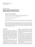
The nonlinear effects that are not taken care of in the
linear model are put into a model to be handled by a PF.

The resulting linear model (9a) is therefore
x
t+1
=
⎛
⎜
⎜
⎜
⎜
⎜
⎜
⎜
⎜
⎜
⎜
⎜
⎜
⎜
⎜
⎜
⎝
0010
1
2
0
00
010
1
2
0010 1 0

00
010 1
00
001 0
00
000 1
⎞
⎟
⎟
⎟
⎟
⎟
⎟
⎟
⎟
⎟
⎟
⎟
⎟
⎟
⎟
⎟
⎠
x
t
+ f

x
p
t


+ w
t
,
y
= h

x
p
t

+ e
t
,
(14)
and the nonlinear model follows immediately with the above
definitions.
To verify the algorithm numerically the object-oriented
F++ software [15] was used for Monte Carlo simulations
using the above model structure. In Figure 3 the position
RMSE from 100 Monte Carlo simulations for the PF and
the RBPF is depicted using N
= 2000 particles. The
computational complexity for RBPF versus PF for the
describedsystemisanalyzedindetailin[23], and not part
of this paper. As seen, the RBPF RMSE is slightly lower than
the PF’s, in accordance with the observations made in [23].
6. Conclusions
This paper presents the Rao-Blackwellized particle filter
(RBPF) in a new way that can be interpreted as a Kalman

filter bank with stochastic branching and pruning. The
proposed Algorithm 2 contains only standard Kalman filter
operations, in conrtast to the state-of-the-art implementa-
tion in Algorithm 1 (where step 4(c) is nonstandard). On the
practical side, the new algorithm facilitates code reuse and
is better suited for object-oriented implementations. On the
theoretical side, we have pointed out that an extension to a
square root implementation of the KF is straightforward in
the new formulation. A related and interesting task for future
resarch is to extend the RBPF to smoothing problems, where
the new algorithm should also be quite attractive.
Appendices
A. Derivation of Filter Bank RBPF
In this appendix, the RBPF formulation found in Algorithm
2 is derived. The initialization of the filter is treated first,
then the measurement update step, the time update step, and
finally the resampling.
A.1. Initialization. To initialize the filtering recursion, the
distribution
p

x
k
0
, X
p
0
| Y
−1


=
p

x
k
0
| X
p
0
, Y
−1

p

X
p
0
| Y
−1

(A.1)
is assumed known, where p(x
k
0
| X
p
0
, Y
−1
) should be analyti-

cally tractable for best result and
Y
−1
can be interpreted as no
measurements. This state is represented by a set of par ticles,
with matching covariance matrices and weights,
x
(i)
0
|−1
=
⎛
⎝
x
p(i)
0
|−1
x
k(i)
0
|−1
⎞
⎠
, P
(i)
0
|−1
=
⎛
⎝

00
0 P
k(i)
0|−1
⎞
⎠
ω
(i)
0
|−1
,(A.2)
where the particles are chosen from the distribution for
x
p
and ω
(i)
represents the particle weight. Here, x
p
is
point distributed, hence the singular covariance matrix.
Furthermore, the value of x
k
depends on the specific x
p
.
For the given model, draw N independent and identically
distributed (IID) samples x
p(i)
0
|−1

∼ p(x
p
0
), set ω
0|−1
= N
−1
,
and compose the combined state vectors as
x
(i)
0
|−1
=
⎛
⎝
x
p(i)
0
|−1
x
k
0
|−1
⎞
⎠
, P
(i)
0
|−1

=
⎛
⎝
00
0 Π
k
0
|−1
⎞
⎠
. (A.3)
This now gives an initial state estimate with a representation
similar to Figure 1(c).
A.2. Measurement Update. The next s tep is to introduce
information from the measurement y
t
into the posterior
distributions in (A.1), or more generally,
p

x
k
t
, X
p
t
| Y
t−1

=

p

x
k
t
| X
p
t
, Y
t−1

p

X
p
t
| Y
t−1

. (A.4)
8 EURASIP Journal on Advances in Signal Processing
First, conditioned on the particle state, the measurement can
be introduced into the left factor,
p

x
k
t
| X
p

t
, Y
t

=
p

y
t
| X
p
t
, x
k
t
, Y
t−1

p

x
k
t
| X
p
t
, Y
t−1

p


y
t
| X
p
t
, Y
t−1

=
p

y
t
| x
p
t
, x
k
t

p

x
k
t
| X
p
t
, Y

t−1

p

y
t
| X
p
t
, Y
t−1

,
(A.5a)
where the denominator acts as a normalizing factor that in
the end does not have to be computed explicitly. The last
equality follows from (7b).
Resorting to the special case of the given model (assum-
ing the
X
p
t
matches the history or system mode of particle i
indicated by
(i)
),
p

x
k

t
| X
p
t
, Y
t

=
N

y
t
; y
(i)
t
, R

·
N

x
k
t
; x
k(i)
t|t−1
, P
k(i)
t|t−1


p

y
t
| Y
t−1
, X
p
t

=
N

x
k
t
|t
; x
k(i)
t
|t
, P
k(i)
t
|t

(A.5b)
with
x
(i)

t
|t
= x
(i)
t
|t−1
+ K
(i)
t

y
t
− y
(i)
t

, (A.5c)
P
(i)
t
|t
= P
(i)
t
|t−1
− K
(i)
t
S
(i)

t
K
(i)T
t
, (A.5d)
y
(i)
t
= H
(i)
t
|t−1
x
(i)
t
|t−1
+ h

x
p(i)
t
|t−1

,
K
(i)
t
= P
(i)
t|t−1

H
(i)T
t

S
(i)
t

−1
,
S
(i)
t
= H
(i)
t
P
(i)
t
|t−1
H
(i)T
t
+ R.
(A.5e)
This should be recognized as a standard Kalman filter
measurement update. The second factor of (A.4)canbe
handled in a similar way
p


X
p
t
| Y
t

=
p

y
t
| X
p
t
, Y
t−1

p

X
p
t
| Y
t−1

p

y
t
| Y

t−1

=

p

y
t
| X
p
t
, x
k
t
, Y
t−1

p

x
k
t
| X
p
t
, Y
t−1

dx
k

t
·
p

X
p
t
| Y
t−1

p

y
t
| Y
t−1

=

p

y
t
| x
k
t
, x
p
t


p

x
k
t
| X
p
t
, Y
t−1

dx
k
t
p

X
p
t
| Y
t−1

p

y
t
| Y
t−1

,

(A.6a)
where the marginalization in the middle step is used to bring
out the structure needed and the last equality uses (7b).
The particle filter part of the state space is handled using
p

X
p
t
| Y
t

=
p

X
p
t
| Y
t−1

p

y
t
| Y
t−1

·


N

y
t
; y
(i)
t
, R

N

x
k
t
; x
k(i)
t
|t−1
, P
k(i)
t
|t−1

dx
k
t
=
p

X

p
t
| Y
t−1

p

y
t
| Y
t−1

·
N

y
t
; y
(i)
t
, H
(i)
t
P
(i)
t
|t−1
H
(i)T
t

+ R

,
(A.6b)
which is used to update the part icle weights
ω
(i)
t
|t
∝ N

y
t
; y
(i)
t
, H
(i)
t
P
(i)
t
|t−1
H
(i)T
t
+ R

ω
(i)

t
|t−1
. (A.6c)
This gives
p

x
k
t
, X
p
t
| Y
t

=
p

x
k
t
| X
p
t
, Y
t

p

X

p
t
| Y
t

. (A.6d)
A.3. Time Update and Pruning. To predict the state in the next
time instance the first step is to derive p(x
p
t+1
, x
k
t+1
| X
p
t
, Y
t
)
and then condition on x
p
t+1
. This turns (5a) into the following
two steps:
p

x
t+1
| X
p

t
, Y
t

=
p

x
p
t+1
, x
k
t+1
| X
p
t
, Y
t

=

p

x
p
t+1
, x
k
t+1
| X

p
t
, x
k
t
, Y
t

p

x
k
t
| X
p
t
, Y
t

dx
k
t
=

p

x
p
t+1
, x

k
t+1
| x
p
t
, x
k
t

p

x
k
t
| X
p
t
, Y
t

dx
k
t
,
(A.7a)
where (7a) has been used in the last step. With the
given model structure and the same assumption about
X
p
t

matching particle i
p

x
t+1
| X
p
t
, Y
t

=

p
(
x
t+1
| x
t
)
p

x
k
t
| X
p
t
, Y
t


dx
k
t
=

N

x
t+1
; x

(i)
t+1
|t
, P

(i)
t+1
|t

N

x
k
t
; x
k(i)
t
|t

, P
k(i)
t
|t

dx
k
t
= N

x
t+1
; F
(i)
t
x
(i)
t
|t
+ f

x
p(i)
t

, F
(i)
t
P
(i)

t
|t
F
(i)T
t
+ G
(i)
t
QG
(i)T
t

,
(A.7b)
where the primed variables (and hence the whole time
update step) can be obtained using a Kalman filter time
update for each particle,
x

(i)
t+1
|t
= F
(i)
t
|t
x
(i)
t
|t

+ f

x
p(i)
t

,
(A.7c)
P

(i)
t+1
|t
= F
(i)
t
|t
P
(i)
t
|t
F
(i)T
t
|t
+ G
(i)
t
|t
QG

(i)T
t
|t
.
(A.7d)
EURASIP Journal on Advances in Signal Processing 9
The result uses the initial Gaussian assumption, as well as the
Markov property in (7a). The last step follows immediately
when only Gaussian distributions are involved. The result
can either be directly recognized as a Kalman filter time
update step or be derived through straightforward but
lengthy calculations.
Note that this updates the x
p
part of the state vector as
if it was a regular part of the state. As a result, x no longer
has a point distribution in the x
p
dimension; instead, the
distribution is now a Gaussian mixture.
Conditioning on x
p
t+1
(pruning of the continuous x
p
t+1
to
samples again) follows immediately as
p


x
k
t+1
| X
p
t+1
, Y
t

=
p

x
t+1
| X
p
t+1
, Y
t

=
p

x
p
t+1
| x
t+1
, X
p

t
, Y
t

p

x
t+1
| X
p
t
, Y
t

p

x
p
t+1
| X
p
t
, Y
t

=
p

x
p

t+1
| x
p
t+1

p

x
t+1
| X
p
t
, Y
t

p

x
p
t+1
| X
p
t
, Y
t

=
p

x

t+1
| X
p
t
, Y
t

p

x
p
t+1
| X
p
t
, Y
t

.
(A.7e)
Once again, looking at the special case of the model with
linear-Gaussian substructure it is now necessary to choose
new particles x
p
t+1
. Conveniently enough, the distribution
p(x
p
t+1
| X

p
t
, Y
t
) is available as a marginalization, yielding
p

x
k
t+1
| X
p
t+1
, Y
t

=
N

x
p
t+1
, x
k
t+1
; x

t+1|t
, P


t+1|t

p

x
p
t+1
| X
p
t
, Y
t

. (A.7f)
This can be identified as a measurement update in a Kalman
filter, where the newly selected particles become virtual
measurements without measurement noise. Once again, this
can be verified with straightforward, but quite lengthy,
calculations. The measurement is called virtual because it is
mathematically motivated and based on the information in
the state rather than an actual measurement.
The second factor of (6) can then be handled directly,
using a particle filter time update step and the result
in (A.7b). This at the same time provides the vir tual
measurements needed for the above step.
Note that the conditional separation still holds so that
p

x
k

t+1
, X
p
t+1
| Y
t

=
p

x
k
t+1
| X
p
t+1
, Y
t

p

X
p
t+1
| Y
t

,
(A.8)
where the first factor comes from (A.7f) and the second is

provided by the time update of the PF. This form is still
suitable for a Rao-Blackwellized measurement update.
The particle filter step and the conditioning on x
p
t+1
can
now be combined into the following virtual measurement
update:
x
(i)
t+1
|t
= x

(i)
t+1
|t
+ P

(i)
t+1
|t
H


H

P

(i)

t+1
|t
H

(i)T

−1
×

ξ
(i)
t+1
− H

x

(i)
t+1
|t

,
P
(i)
t+1
|t
= P

(i)
t+1
|t

− P

(i)
t+1
|t
H

T

H

P

(i)
t+1
|t
H

T

−1
H

P

(i)
t
|t
,
(A.9)

where H

=

I 0

and x

, P

are defined in (A.7c)-(A.7d).
The vir tual measurements are chosen from the Gaussian
distribution given by
ξ
(i)
t+1
∼ N

H

x

(i)
t+1
|t
, H

P

(i)

t+1
|t
H

T

. (A.10)
After this step x
p
is once again a point distribution x
p(i)
t+1
|t
=
ξ
(i)
t+1
and P
(i)
t+1|t
is zero except for P
k(i)
t+1|t
. The particle filter
update and the compensation for the selected particle have
been done in one step. Taking this structure into account
it is possible to obtain a more efficient implementation,
computing just x
k
t+1

|t
and P
k
t+1
|t
.
If another different proposal density for the particle
filter is more suitable, this is easily incorporated by simply
changing the distribution of ξ
t+1
and then appropriately
compensating the weights for this.
This completes the recursion; however, resampling is still
needed for this to work in practice.
A.4. Resampling. As with the particle filter, if the described
RBPF is r un with exactly the steps described above it will
end up with all the particle weight in one single par ticle.
This degrades estimation performance. The solution is [1]
to randomly get rid of unimportant particles and replace
them with more l ikely ones. In the RBPF this is done in
exactly the same way as described for the particle filter, with
the difference that when a particle is selected, so is the full
state matching that particle, as well as the covariance matrix
describing the Kalman filter part of the state. The idea is to
select new particles such that
Pr

x
(i)
+

= x
( j)

=
ω
( j)
, (A.11)
that is, drawing samples with replacement. T he new weight
of each particle is now ω
(i)
+
= N
−1
,whereN is the number of
particles.
Acknowledgments
Dr. G. Hendeby would like to acknowledge the support from
the European 7th framework project Cog nito ( ICT-248290).
All authors are greatful for support from the Swedish
Research Council via a project grant and its Linnaeus
Excellence Center CADICS. The authors would also like to
thank the reviewers for many and valuable comments that
have helped to improve this paper.
10 EURASIP Journal on Advances in Signal Processing
References
[1]N.J.Gordon,D.J.Salmond,andA.F.M.Smith,“Novel
approach to nonlinear/non-Gaussian Bayesian state estima-
tion,” IEE Proceedings F: Radar and Signal Processing, vol. 140,
no. 2, pp. 107–113, 1993.
[2]A.Doucet,N.deFreitas,andN.Gordon,Eds.,Sequential

Monte Carlo Methods in Practice, Statistics for Engineeringand
Information Science, Springer, New York, NY, USA, 2001.
[3] R. E. Kalman, “A new approach to linear filtering and
prediction problems,” Journal Basic Engieering, Ser ies D, vol.
82, pp. 35–45, 1960.
[4] T. Kailat, A. H. Sayed, and B. Hassibi, Linear Estimation,
Prentice-Hall, Englewood Cliffs, NJ, USA, 2000.
[5] A. Doucet, S. Godsill, and C. Andrieu, “On sequential Monte
Carlo sampling methods for Bayesian filtering,” Statistics and
Computing, vol. 10, no. 3, pp. 197–208, 2000.
[6] G. Casella and C. P. Robert, “Rao-blackwellisation of sampling
schemes,” Biometrika, vol. 83, no. 1, pp. 81–94, 1996.
[7] A. Doucet, N. J. Gordon, and V. Krishnamurthy, “Particle
filters for state estimation of jump Markov linear systems,”
IEEE Transactions on Signal Processing, vol. 49, no. 3, pp. 613–
624, 2001.
[8] R. Chen and J. S. Liu, “Mixture Kalman filters,” Journal of the
Royal Statistical Society. Series B, vol. 62, no. 3, pp. 493–508,
2000.
[9] C. Andrieu and A. Doucet, “Particle filtering for partially
observed Gaussian state space models,” Journal of the Royal
Statistical Society. Series B, vol. 64, no. 4, pp. 827–836, 2002.
[10] T. Sch
¨
on, F. Gustafsson, and P. J. Nordlund, “Marginalized
particle filters for mixed linear/nonlinear state-space models,”
IEEE Transactions on Signal Processing, vol. 53, no. 7, pp. 2279–
2289, 2005.
[11] T. B. Sch
¨

on, R. Karlsson, and F. Gustafsson, “The marginalized
particle filter in practice,” in Proceedings of IEEE Aerospace
Conference, Big Sky, Mont, USA, March 2006.
[12] O. Capp
´
e, S. J. Godsill, and E. Moulines, “An overview of
existing methods and recent advances in sequential Monte
Carlo,” Proceedings of the IEEE, vol. 95, no. 5, pp. 899–924,
2007.
[13] R. Morales-Men
´
endez, N. de Freitas, and D. Poole, “Real
time monitoring of complex industrial processes with particle
filters,” in Advances in Neural Information Processing Systems
15, pp. 1457–1464, Vancouver, Canada, 2002.
[14] N. de Freitas, R. Dearden, F. Hutter, R. Morales-Men
´
endez,
J. Mutch, and D. Poole, “Diagnosis by a waiter and a Mars
explorer ,” Proceedings of the IEEE, vol. 92, no. 3, pp. 455–468,
2004.
[15] G. Hendeby and R. Karlsson, “Target tracking performance
evaluation—a general software environment for filtering,” in
Proceedings of IEEE Aerospace Conference, Big Sky, Mont, USA,
March 2007.
[16] V.
ˇ
Sm
´
ıdl, “Software analysis unifying particle filtering and

marginalized particle filter ing,” in Proceedings of the 13th IEEE
International Conference on Information Fusion, Edinburgh,
UK, July 2010.
[17] D. L. Alspach and H. W. Sorenson, “Nonlinear Bayesian
estimation using Gaussian sum approximations,” IEEE Trans-
actions on Automatic Control
, vol. 17, no. 4, pp. 439–448, 1972.
[18] H. W. Sorenson and D. L. Alspach, “Recursive bayesian
estimation using gaussian sums,” Automatica,vol.7,no.4,pp.
465–479, 1971.
[19] H. A. P. Blom and Y. Bar-Shalom, “Interacting multiple model
algorithm for systems with Markovian switching coefficients,”
IEEE Transactions on Automatic Cont rol,vol.33,no.8,pp.
780–783, 1988.
[20] C. R. Rao, “Information and the accuracy attainable in the
estimation of statistical parameters,” Bulletin of the Calcutta
Mathematical Society, vol. 37, pp. 81–91, 1945.
[21] D. Blackwell, “Conditional expectation and unbiased sequen-
tial estimation,” The Annals of Mathematical Statistics, vol. 18,
no. 1, pp. 105–110, 1947.
[22] E. L. Lehmann, Theory of Point Estimation, Probabilityand
Mathematical Statistics, John Wiley & Sons, New York, NY,
USA, 1983.
[23] R. Karlsson, T. Sch
¨
on, and F. Gustafsson, “Complexity analysis
of the marginalized particle filter,” IEEE Transactions on Signal
Processing, vol. 53, no. 11, pp. 4408–4411, 2005.
[24] F. Gustafsson, F. Gunnarsson, N. Bergman et al., “Particle
filters for positioning, navigation, and tracking,” IEEE Trans-

actionsonSignalProcessing, vol. 50, no. 2, pp. 425–437, 2002.
[25] R. Karlsson and F. Gustafsson, “Recursive Bayesian estimation:
bearings-only applications,” IEE Proceedings F: Radar and
Sonar Navigation, vol. 152, no. 5, pp. 305–313.
[26] T. Sch
¨
on, R. Karlsson, and F. Gustafsson, “The marginalized
particle filter—analysis, applications and generalizations,” in
Workshop on Sequential Monte Carlo Methods: Filtering and
Other Applications, Oxford, UK, July 2006.
[27] D. T
¨
ornqvist,T.B.Sch
¨
on, R. Karlsson, and F. Gustafsson,
“Particle filter SLAM with hig h dimensional vehicle model,”
Journal of Intelligent and Robotic Systems,vol.55,no.4-5,pp.
249–266, 2009.
[28] R. Karlsson and F. Gustafsson, “Particle filter for underwater
terrain navigation,” in IEEE Statistical Signal Processing Work-
shop, pp. 526–529, St. Louis, Mo, USA, Oct. 2003.
[29] N. Svenzen, Real time map-aided positioning using a Bayesian
approach, M.S. thesis, Department of Electrical Engineering.
Link
¨
oping University, Link
¨
oping, Sweden, 2002.
[30] R. Karlsson, T. B. Sch
¨

on, D. T
¨
ornqvist,G.Conte,andF.
Gustafsson, “Utilizing model structure for efficient simulta-
neous localization and mapping for a UAV application,” in
Proceedings of IEEE Aerospace Conference, Big Sky, Mont, USA,
March 2008.
[31] P J. Nordlund, Sequential Monte Carlo filters and integrated
navigation, M.S. thesis, Department of Electrical Engineering,
Link
¨
opings Universitet, Link
¨
oping, Sweden, May 2002.
[32] G. Hendeby, Performance and impleme ntation aspects of non-
linear filtering, M.S. thesis, Link
¨
oping Studies in Science and
Technology, March 2008.