Báo cáo hóa học: " Research Article Hidden Markov Model with Duration Side Information for Novel HMMD Derivation, with Application to Eukaryotic Gene Finding" docx

Hindawi Publishing Corporation
EURASIP Journal on Advances in Signal Processing
Volume 2010, Article ID 761360, 11 pages
doi:10.1155/2010/761360
Research Article
Hidden Markov M odel with Duration Side Information for Novel
HMMD Derivation, with Application to Eukaryotic Gene Finding
S. Winters-Hilt,
1, 2
Z. Jiang,
1
and C. Baribault
1
1
Department of Computer Science, University of New Orleans, 2000 Lakeshore Drive, New Orleans, LA 70148, USA
2
Research Institute for Children, Children’s Hospital, New Orleans, LA 70118, USA
Correspondence should be addressed to S. Winters-Hilt,
Received 25 March 2010; Revised 10 July 2010; Accepted 27 September 2010
Academic Editor: Haris Vikalo
Copyright © 2010 S. Winters-Hilt et al. This is an open access article distributed under the Creative Commons Attribution License,
which permits unrestricted use, distribution, and reproduction in any medium, provided the original work is properly cited.
We describe a new method to introduce duration into an HMM using side information that can be put in the form of a martingale
series. Our method makes use of ratios of duration cumulant probabilities in a manner that meshes with the column-level dynamic
programming construction. Other information that could be incorporated, via ratios of sequence matches, includes an EST and
homology information. A familiar occurrence of a martingale in HMM-based efforts is the sequence-likelihood ratio classification.
Our method suggests a general procedure for piggybacking other side information as ratios of side information probabilities, in
association (e.g., one-to-one) with the duration-probability ratios. Using our method, the HMM can be fully informed by the side
information available during its dynamic table optimization—in Viterbi path calculations in particular.
1. Introduction
Hidden Markov models have been extensively used in speech

recognition since the 1970s and in bioinformatics since the
1990s. In automated gene finding, there are two types of ap-
proaches based on data intrinsic to the genome under study
or extrinsic to the genome (e.g., homology and EST data).
Since around 2000, the best gene finders have been based
on combined intrinsic/extrinsic statistical modeling [1].
The most common intrinsic statistical model is an HMM,
so the question naturally arises—how to incorporate side
information into an HMM? We resolve that question in this
paper by treating duration distribution information its elf
as side information and demonstrate a process for incor-
porating that side information into an HMM. We thereby
bootstrap from an HMM formalism to a HMM-with-
duration (more generally, a hidden semi-Markov model or
HSMM). Our method for incorporating side information
incorporates duration information precisely as needed to
yield an HMMD. In what follows, we apply this capability to
actual gene finding, where model sophistication in the choice
of emission variables is used to obtain a highly accurate ab
initio gene finder.
The original description of an explicit HMMD required
computation of order O(TNN + TND
2
)[2], where T is the
period of observations, N is the number of states, and D is
the maximum duration of state transitions to self allowed
in the model (where D is typically >500 in gene-structure
identification and channel-current analysis [3]). This is
generally too prohibitive (computationally expensive) in
practical operations and introduces a severe maximum-

interval constraint on the self-transition distribution model.
Improvements via hidden semi-Markov models to com-
putations of order O(TNN + TND) were described in
[4, 5], where the Viterbi and Baum-Welch algorithms
were implemented, the latter improvement only obtained
as of 2003. In these derivations, however, the maximum-
interval constraint is still present (comparisons of these
methods were subsequently detailed in [6]). Other HMM
generalizations include factorial HMMs [7] and hierarchical
HMMs [8]. For the latter, inference computations scaled
as O(T
3
) in the original description and have since been
improved to O(T)by[9]. The above HMMD variants all
have a computational inefficiency problem which limits their
applications in real-world settings. In [10], a hidden Markov
model with binned duration (HMMBD) is shown to be
2 EURASIP Journal on Advances in Signal Processing
possible with computation complexity of O(TNN + TND
∗
),
where D
∗
is typically <50 (and can often be as small as
4 or 5, as in the application that follows). These bins are
generated by analyzing the state-duration distribution and
grouping together neighboring durations if their differences
are below some cutoff. In this way, we now have an efficient
HMM with duration model that can be applied in many areas
that were originally thought impractical. Furthermore, the

binning allows us to have a “tail bin” and thereby eliminate
the maximum duration restriction.
In DNA sequence analysis, the observation sequences
consist of the nucleotide bases: adenine, thymine, cytosine,
and guanine
{A, T, C, G}, and the hidden states are labels
associated with regions of exon, intron, and junk
{e, i, j}.
In gene finding, the hidden Markov models usually have
to be expanded to include additional requirements, such
as the codon frame information, site-specific statistics, and
state-duration probability information, and must also follow
some exception rules. For example, the start of an initial
exon typically begins with “ATG”, final exons end with a
stop codon
{TAA, TAG, TGA}, and the introns generally
follow the GT-AG rule. There are many popular gene finder
application programs: AUGUSTUS, Gene Mark, GeneScan,
Genie, and so forth [11]. The statistical models employed
by Gene Mark and AUGUSTUS involve implementations or
approximations of an HMM with duration (HMMD), where
state durations are not restricted to be geometric, as in the
standard HMM modeling (further details are given in the
background section to follow). For the Gene Mark HMMD,
the state-duration distributions are an estimation of the
length distributions from the training set of sequences, and
are characterized by the minimum and maximum duration
length allowed. For example, the minimum and maximum
durations of introns and intergenic sequences are set to
20 and 10,000 nts. For the AUGUSTUS HMMD, an intron

submodel is introduced on durations [12], providing an
approximate HMMD modeling on the introns (but not
exons, etc.). The improvement to HMMD modeling on the
introns is critical to an HMM-based gene finder that can
be used in “general use” situations, such as applications to
raw genomic sequence (not preprocessed situations, such as
one coding sequence in a selected genomic subsequence, as
discussedin[13]). The hidden Markov model with binned
duration (HMMBD) algorithm, presented in [10], offers a
significant reduction in computational time for all HMMD-
based methods, to approximately the computational time of
the HMM-process alone, while not imposing a maximum
duration cutoff, and is used in the implementations and
tuning described here. In adopting any model with “more
parameters”, such as an HMMD over an HMM, there is
potentially a problem with having sufficient data to support
the additional modeling. This is generally not a problem
in any HMM model that requires thousands of samples
of nonself transitions for sensor modeling, however, since
knowing the boundary positions allows the regions of self-
transitions (the durations) to be extracted with similar high
sample number as well, for effective modeling of the
duration distributions in the HMMD (as will be the case
in the genomics analysis to follow).
The breadth of applications for HMMs goes beyond
the aforementioned to include gesture recognition [14, 15],
handwriting and text recognition [16–19], image process-
ing [20, 21], computer vision [22], communication [23],
climatology [24], and acoustics [25, 26]tolistafew.
HMMs are a central method in all of these approaches

not because they are the simplest, most efficient, modeling
approach that is obtained when one combines a Bayesian
statistical foundation for stochastic sequential analysis with
the efficient dynamic programming table constructions
possible on a computer. As mentioned above, in many
applications, the ability to incorporate the state duration
into the HMM is very important because the standard,
HMM-based, the Viterbi, and Baum-Welch algorithms are
otherwise critically constrained in their modeling ability to
distributions on state intervals that are geometric. This can
lead to a significant decoding failure in noisy environments
when the state-interval distributions are not geometric
(or approximately geometric). The starkest contrast occurs
for multimodal distributions and heavy-tailed distributions.
Critical improvement to overall HMM application rests
not only with generalization to HMMD, however, but also
to a generalized, fully interpolated, clique HMM, the
“meta-HMM” described in [27], and also with the ability
to incorporate external information, “side-information”, into
the HMM, as described in this paper.
2. Background
2.1. Markov Chains and Standard Hidden Markov Models. A
Markov chain is a sequence of random variables S
1
; S
2
; S
3
;
with the Markov property of limited memory, where a first-

order Markov assumption on the probability for observing a
sequence “s
1
s
2
s
3
s
4
···s
n
”is
P
(
S
1
= s
1
, , S
n
= s
n
)
,
= P
(
S
1
= s
1

)
P
(
S
2
= s
2
| S
1
= s
1
)
···
×
P
(
S
n
= s
n
| S
n−1
= s
n−1
)
.
(1)
In the Markov chain model, the states are also the observ-
ables. For a hidden Markov model (HMM), we generalize
to where the states are no longer directly observable (but

still 1st-order Markov), and for each state, say S
1
,wehave
a statistical linkage to a random variable, O
1
, that has an
observable base emission, with the standard (0th-order)
Markov assumption on prior emissions (see [27]forclique-
HMM generalizations). The probability for observing base
sequence “b
1
b
2
b
3
b
4
···b
n
” with state sequence taken to be
“s
1
s
2
s
3
s
4
···s
n

” is then
P
(
O; S
)
= P

“b
1
b
2
b
3
b
4
···b

n
;“s
1
s
2
s
3
s
4
···s

n


=
P
(
S
1
= s
1
)
P
(
S
2
= s
2
| S
1
= s
1
)
···
×
P
(
S
n
= s
n
| S
n−1
= s

n−1
)
× P
(
O
1
= b
1
S
1
= s
1
)
···P
(
O
n
= b
n
| S
n
= s
n
)
.
(2)
EURASIP Journal on Advances in Signal Processing 3
AhiddenMarkovmodelisa“doublyembeddedstochastic
process with an underlying stochastic process that is not
observable, but can only be observed through another

set of stochastic process that produce the sequence of
observations” [25].
2.2. HMM with Duration Modeling. In the standard HMM,
when a state i is entered, that state is occupied for a period of
time, via self-transitions, until transiting to another state j.If
the state interval is given as d, the standard HMM description
of the probability distribution on state intervals is implicitly
given by
p
i
(
d
)
= a
d−1
ii
(
1
− a
ii
)
,(3)
where a
ii
is self-transition probability of state i. This
geometric distribution is inappropriate in many cases. The
standard HMMD replaces (3)withap
i
(d) that models the
real duration distribution of state i. In this way, explicit

knowledge about the duration of states is incorporated into
the HMM. A general HMMD can be illustrated as
p
i
(d)
a
ij
a
ji
s
i
p
j
(d)
s
j
When entered, state i will have a duration of d according
to its duration density p
i
(d), and it then transits to another
state j according to the state transition probability a
ij
(self-
transitions, a
ii
, are not permitted in this formalism). It is
easy to see that the HMMD will turn into an HMM if p
i
(d)
is set to the geometric distribution shown in (3). The first

HMMD formulation was studied by Ferguson [2]. A detailed
HMMD description was later given by [28](wefollowmuch
of the [28] notation in what follows). There have been
many efforts to improve the computational efficiency of the
HMMD formulation given its fundamental utility in many
endeavors in science and engineering. Notable amongst these
are the variable transition HMM methods for implementing
the Viterbi algorithm introduced in [4] and the hidden semi-
Markov model implementations of the forward-backward
algorithm [5].
2.3. Significant Distributions That Are Not Geometric. Non-
geometric duration distributions occur in many familiar
areas, such as the length of spoken words in phone conversa-
tion, as well as other areas in voice recognition. The Gaussian
distribution occurs in many scientific fields, and there are
huge number of other (skewed) types of distributions, such
as heavy-tailed (or long-tailed) distributions and multimodal
distributions.
Heavy-tailed distributions are widespread in describing
phenomena across the sciences [29]. The log-normal and
Pareto distributions are heavy-tailed distributions that are
almost as common as the normal and geometric distribu-
tions in descriptions of physical phenomena or man-made
phenomena and many other phenomena. Pareto distribution
was originally used to describe the allocation of wealth of
the society, known as the famous 80–20 rule; namely, about
80% of the wealth was owned by a small amount of people,
while “the tail”, the large part of people only have the rest
20% wealth [30]. Pareto distribution has been extended to
many other areas. For example, internet file-size trafficis

a long-tailed distribution; that is, there are a few large-
sized files and many small-sized files to be transferred. This
distribution assumption is an important factor that must
be considered to design a robust and reliable network and
Pareto distribution could be a suitable choice to model such
traffic. (Internet applications have found more and more
heavy-tailed distribution phenomena.) Pareto distribution’s
can also be found in a lot of other fields, such as economics.
Log-normal distributions are used in geology and min-
ing, medicine, environment, atmospheric science, and so on,
where skewed distribution occurrences are very common
[29]. In Geology, the concentration of elements and their
radioactivity in the Earth’s crust are often shown to be log-
normaly distributed. The infection latent period, the time
from being infected to disease symptoms occurs, is often
modeled as a log-normal distribution. In the environment,
the distribution of particles, chemicals, and organisms is
often log-normal distributed. Many atmospheric physical
and chemical properties obey the log-normal distribution.
The density of bacteria population often follows the log-
normaly distribution law. In linguistics, the number of
letters per words and the number of words per sentence
fit the log-normal distribution. The length distribution for
introns, in particular, has very strong support in an extended
heavy-tail region, likewise for the length distribution on
exons or open reading frames (ORFs) in genomic DNA
[31, 32]. The anomalously long-tailed aspect of the ORF-
length distribution is the key distinguishing feature of this
distribution and has been the key attribute used by biologists
using ORF finders to identify likely protein-coding regions in

genomic DNA since the early days of (manual) gene structure
identification.
2.4. Significant Series That Are Martingale. A discrete-time
martingale is a stochastic process where a sequence of
random variables
{X
1
, , X
n
} has conditional expected
value of the next observation equal to the last observation
E(X
n+1
| X
1
, , X
n
) = X
n
,whereE(|X
n
|) < ∞. Similarly,
one sequence, say
{Y
1
, , Y
n
}, is said to be martingale
with respect to another, say
{X

1
, , X
n
},ifforalln :
E(Y
n+1
| X
1
, , X
n
) = Y
n
,whereE(|Y
n
|) < ∞. Examples
of martingales are rife in gambling. For our purposes,
the most critical example is the likelihood-ratio testing in
statistics, with test statistic, the “likelihood ratio”, given
as Y
n
=

n
i=1
g(X
i
)/f(X
i
), where the population densities
considered for the data are f and g. If the better (actual)

distribution is f , then Y
n
is martingale with respect to X
n
.
This scenario arises throughout the HMM Viterbi derivation
if local “sensors” are used, such as with profile HMMs
or position-dependent Markov models in the vicinity of
transition between states. This scenario also arises in the
HMM Viterbi recognition of regions (versus transition out
of those regions), where length-martingale side information
will be explicitly shown in what follows, providing a pathway
for incorporation of any martingale-series side information
4 EURASIP Journal on Advances in Signal Processing
(this fits naturally with the clique-HMM generalizations de-
scribed in [27] as well). Given that the core ratio of cumulant
probabilities that is employed is itself a martingale, this then
provides a means for incorporation of side information in
general.
3. Methods
3.1. The Hidden Semi-Markov Model Via Length Side Infor-
mation. In this section, we present a means to lift side
information that is associated with a region, or transition
between regions, by “piggybacking” that side information
along with the duration side information. We use the
example of such a process for HMM incorporation of
duration itself as the guide. In doing so, we arrive at a hidden
semi-Markov model (HSMM) formalism. (Throughout the
derivation to follow, we try to stay consistent with the
notation introduced by [28].) An equivalent formulation of

the HSMM was introduced in [4] for the Viterbi algorithm
and in [5] for Baum-Welch. The formalism introduced
here, however, is directly amenable to incorporation of side
information and to adaptive speedup (as described in [10]).
For the state duration density p
i
(x = d), 1 ≤ x ≤ D,we
have
p
i
(
x
= d
)
= p
i
(
x
≥ 1
)
·
p
i
(
x
≥ 2
)
p
i
(

x
≥ 1
)
·
p
i
(
x
≥ 3
)
p
i
(
x
≥ 2
)
···
×
p
i
(
x
≥ d
)
p
i
(
x
≥ d − 1
)

·
p
i
(
x
= d
)
p
i
(
x
≥ d
)
,
(4)
where p
i
(x = d) is abbreviated as p
i
(d) if no ambiguity.
Define “self-transition” variable s
i
(d) = probability that next
state is still S
i
, given that S
i
has consecutively occurred d
times up to now
p

i
(
x
= d
)
=
⎡
⎣
d−1

j=1
s
i

j

⎤
⎦
(
1
− s
i
(
d
))
,
where s
i
(
d

)
=
⎧
⎪
⎨
⎪
⎩
p
i
(
x
≥ d +1
)
p
i
(
x
≥ d
)
,if1
≤ d ≤ D − 1,
0, if d
= D.
(5)
We see with comparison of (5)and(3) that we now have
similar form; there are “d
− 1” factors of “s” instead of “a”,
with a “cap term” “(1
− s)” instead of “(1 − a)”, where the
“s” terms are not constant, but only depend on the state’s

duration probability distribution. In this way, “s” can mesh
with the HMM’s dynamic programming table construction
for the Viterbi algorithm at the column level in the same
manner that “a” does. Side information about the local
strength of EST matches or homology matches, and so forth,
that can be put in similar form can now be “lifted” into
the HMM model on a proper, locally optimized Viterbi-
path sense (see Appendices A and B for details). The length
probability in the above form, with the cumulant-probability
ratio terms, is a form of martingale series (more restrictive
than that seen in likelihood ratio martingales).
The derivation of the Baum-Welch and Viterbi HSMM
algorithm, given (5), is outlined in Appendices A and B
(where (A.1)–(B.8) are located). A summary of the Baum-
Welch training algorithm is as follows:
(1) initialize elements (λ)ofHMMD,
(2) calculate b

t
(i, d) using (A.6)and(A.7) (save the two
tables: B
t
(i)andB

t
(i)),
(3) calculate
f
t
(i, d) using (A.4)and(A.5),

(4) re-estimate elements (λ)ofHMMDusing(A.9)–
(A.10),
(5) terminate if stop condition is satisfied, else go to step
(2).
The memory complexity of this method is O(TN). As
shown above, the algorithm first does backward computing
(step (2)) and saves two tables: one is B
t
(i), the other is
B

t
(i). Then, at very time index t, the algorithm can group the
computation of steps (3) and (4) together. So, no forward
tableneedstobesaved.Wecandoaroughestimation
of HMMD’s computation cost by counting multiplications
inside the loops of Σ
T
Σ
N
(which corresponds to the standard
HMM computational cost) and Σ
T
Σ
D
(the additional com-
putational cost incurred by the HMMD). The computation
complexity is O(TN
2
+ TND). In an actual implementation,

a scaling procedure may be needed to keep the forward-
backward variables within a manageable numerical interval.
One common method is to rescale the forward-backward
variables at every time index t using the scaling factor c
t
=
Σ
i
f
t
(i). Here we use a dynamic scaling approach. For this, we
need two versions of θ(k, i, d). Then, at every time index, we
test if the numerical values is too small if so, we use the scaled
version to push the numerical values up; if not, we keep using
the unscaled version. In this way, no additional computation
complexity is introduced by scaling.
As with Baum-Welch, the Viterbi algorithm for the
HMMD is O(TN
2
+ TND). Because logarithm scaling can
be performed for Viterbi in advance; however, the Viterbi
procedure consists only of additions to yield a very fast
computation. For both the Baum-Welch and Viterbi algo-
rithms, use of the HMMBD algorithm [10]canbeemployed
(as in this work) to further reduce computational time
complexity to O(TN
2
), thus obtaining the speed benefits of
a simple HMM, with the improved modeling capabilities of
the HMMD.

3.2. Method for Modeling Gene-Finder State Structure [27]
3.2.1. The Exon Frame States and Other HMM States. Exons
have a 3-base encoding as directly revealed in a mutual
information analysis of gapped base statistical linkages in
prokaryotic DNA, as shown in [3]. The 3-base encoding
elements are called codons, and the partitioning of the exons
into 3-base subsequences is known as the codon framing.
A gene’s coding length must be a multiple of 3 bases. The
term frame position is used to denote one of the 3 possible
positions—0, 1, or 2 by our convention—relative to the first
base of a codon. Introns may interrupt genes after any frame
EURASIP Journal on Advances in Signal Processing 5
position. In other words, introns can split the codon framing
either at a codon boundary or one of the internal codon
positions.
Although there is no need for framing among introns, for
convenience, we associate a fixed frame label with the intron
as a tracking device in order to ensure that the frame of the
following exon transition is constrained appropriately. The
primitive states of the individual bases occurring in exons,
introns, and junk are denoted by
exon states
={e
0
, e
1
, e
2
},
intron states

={i
0
, i
1
, i
2
},
junk state
=

j

.
(6)
The vicinity around the transitions between exon, intron
and junk usually contains rich information for gene identi-
fication. The junk to exon transition usually starts with an
ATG, the exon to junk transition, ends with one of the stop
codons
{TAA, TAG, TGA}. Nearly all eukaryotic introns
start with GT and end with with AG (the AG-GT rule). To
capture the information at these transition areas, we build a
position-dependent emission (pde) table for base positions
around each type of transition point. It is called “position-
dependent” since we make estimation of occurrence of the
bases (emission probabilities) in this area according to their
relative distances to the nearest nonself state transition. For
example, the start codon “ATG” is the first three bases
at the junk-exon transition. The size of the pde region is
determined by a window-size parameter centered at the

transition point (thus, only even numbered window sizes
are plotted in the Results). We use four transition states
to collect such position-dependent emission probabilities
ie; je
0
; ei; e
2
j. Considering the framing information, we
can expand the above four transition into eight transitions
i
2
e
0
; i
0
e
1
; i
1
e
2
; je
0
; e
0
i
0
; e
1
i

1
; e
2
i
2
; e
2
j.Wemakei
2
e
0
; i
0
e
1
;
i
1
e
2
share the same ie emission table and e
0
i
0
; e
1
i
1
; e
2

i
2
share the same ei emission tables. Since we process both
the forward-strand and reverse-strand gene identifications
simultaneously in one pass, there is another set of eight
state transitions for the reverse strand. Forward states and
their reverse state counterparts also share the same emission
table (i.e., their instance counts and associated statistics are
merged). Based on the training sequences’ properties and
the size of the training data set, we adjust the window size
and use different Markov emission orders to calculate the
estimated occurrence probabilities for different bases inside
the window (e.g., interpolated Markov models are used [3]).
The regions on either side of a pde window often include
transcription factor binding sites such as the promoter
for the je window. Statistics from these regions provide
additional information needed to identify start of gene
coding and alternative splicing. The statistical properties in
these regions are described according to zone-dependent
emission (zde) statistics. The signals in these areas can be
very diverse, and their exact relative positions are typically
not fixed positionally. We apply a 5th-order Markov model
on instances in the zones indicated (further refinements
with hash-interpolated Markov models [3] have also met
Junk Exon Intron
3
2 222
1
1
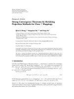
jeeeee eeeeei eiiiiieijejjjjje eeeeee

··· ···
Figure 1: Three kinds of emission mechanisms: (1) position-
dependent emission, (2) hash-interpolated emission, and (3)
normal emission. Based on the relative distance from the state tran-
sition point, we first encounter the position-dependent emissions
(denoted as (1)), then we use the zone-dependent emissions (2),
and finally, we encounter the normal state emissions (denoted as
(3)).
with success but are not discussed further here). The size
of the “zone” region extends from the end of the position-
dependent emission table’s coverage to a distance specified
by a parameter. For the dataruns shown in the Results, this
parameterwassetto50.
There are eight zde tables:
{ieeeee, jeeeee, eeeeei, eeeee j,
eiiiii, iiiiie, ejjjjj,andjjjjje
}, where ieeeee corresponds to
the exon emission table for the downstream side of an ie
transition, with zde region 50 bases wide, for example, the
zone on the downstream side of a non-self transition with
positions in the domain (window, window + 50]. We build
another set of eight hash tables for states on the reverse
strand. We see 2% performance improvement when the zde
regions are separated from the bulk-dependent emissions
(bde), the standard HMM emission for the regions. When
outside the pde and zde regions, thus in a bde region, there
are three emission tables for both the forward and reverse
strands exon, intron, and junk states, corresponding to the
normal exon emission table, the normal intron emission
table and the normal junk emission table. The three kinds

of emission processing are shown in Figure 1.
The model contains the following 27 states in total
for each strand, three each of
{ieeeee, jeeeee, eeeeei, eeeee j,
eeeeee, eiiiii, iiiiie, iiiiii
}, corresponding to the different read-
ing frames, and one each of
{ejjjjj, jjjjje,andjjjjjj}.
As before, there is another set of corresponding reverse-
strand states, with junk as the shared state. When a state
transition happens, junk to exon for example, the positional-
dependent emissions inside the window ( je)willberef-
erenced first, then the state travels to the zone-dependant
emission zone ( jeeeee), then travels to the state of the normal
emission region (eeeee), then travels to another state of
zone-dependent emissions (eeeeei or eeeee j), then to a bulk
region of self-transitions (iiiiiii or jjjjjj), and so forth,
The duration information of each state is represented by
the corresponding bin assigned by the algorithm, according
to [10]. For convenience in calculating emissions in the
Viterbi decoding, we precompute the cumulant emission
tables for each of 54 substates (states of the forward and
reverse strand), then as the state transitions, its emission
contributions can be determined by the differences between
two references to the precomputed cumulant array data.
6 EURASIP Journal on Advances in Signal Processing
The occurrence of a stop codon (TAA, TAG, or TGA)
that is in reading frame 0 and located inside an exon, or
across two exons because of the intron interruption, is called
as an “in-frame stop”. In general, the occurrences of in-

frame stops are considered very rare. We designed our in-
frame stop filter to penalize such Viterbi paths. A DNA
sequence has six reading frames (read in six ways based on
frames), three for the forward strand and three for the reverse
strand. When precomputing the emission tables in the above
for the sub-states, for those sub-states related to exons we
consider the occurrences of in-frame stop codons in the six
reading frames. For each reading frame, we scan the DNA
sequence from left to the right, and whenever a stop codon
is encountered in-frame, we add to the emission probability
for that position a user defined stop penalty factor. In this
way, the in-frame stop filter procedure is incorporated into
the emission table building process and does not bring the
additional computational complexity to the program. The
algorithmic complexity of the whole program is O(TND
∗
)
where N
= 54 sub-states and D
∗
is the number of bins for
each sub-state, and the memory complexity is O(TN), via
the HMMBD method described in [10].
3.3. Hardware Implementation. The whole program for this
application is written in the C programming language. The
GNU Compiler Collection (GCC) is used to compile the
codes. The Operating system used is Ubuntu/Linux, running
on a server with 8 GB RAM. In general, the measure of pre-
diction performance is taken at both individual nucleotide
level and the full exon level, according to the specification in

[33], where we calculate sensitivity (SN), specificity (SP), and
take their average as our final accuracy rate (AC).
3.4. Prediction Accuracy Measures. The sensitivity (SN),
specificity (SP), and accuracy (AC) are defined at the base
or nucleotide level, or complete exon match level
SN
=
TP
[
TP + FN
]
,SP
=
TP
[
TP + FP
]
,AC
=
(
SN + SP
)
2
,
(7)
where TP: true positive count; FN: false negative count; and
FP: false positive count.
3.5. Data Preparation. The data we use in the experiment are
Chromosomes I–V of C. elegans that were obtained from
release WS200 of Wormbase [34]. The data preparation is

describedin[27] and is done exactly the same in order to
perform a precise comparison with the meta-HMM method.
The reduced data set, without the coding regions that
have (known) alternative splicing, or any kind of multiple
encoding, is summarized in Tables 1 and 2.
4. Results
We take advantage of the parallel presentation in [27]to
start the tuning with a parameter set that is already nearly
optimized (i.e., the Markov emissions, window size, and
other genome-dependent tuning parameters is already close
0.4
0.5
0.6
0.7
0.8
0.9
1
Accuracy
0 2 4 6 8 101214161820
Window size
Nucleotide accuracies
M
= 8
M
= 5
M
= 2
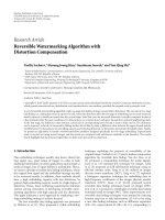
Figure 2: Nucleotide level accuracy rate results with Markov order
of 2, 5, and 8, respectively, for C. elegans, Chromosomes I–V.
to optimal). For verification purposes, we first do training

and testing using the same folds, the results for each of
the five folds indicated above are very good, a 99%-100%
accuracy rate (not shown). We then do a “proper” single
train/test fold from the fivefold cross-validation set (i.e., folds
1–4 to train, and the 5th fold as test), and explore the tuning
on Markov model and window size as shown in Figures 2–
5. We then perform a complete fivefold cross-validation with
the five folds for the model identified as best (i.e., train on
four folds, test on one, permute over the five holdout test
possibilities and take their average accuracies of the different
train/tests as the overall accuracy).
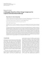
In Figures 2 and 3, we show the results of the experiments
where we tune the Markov order and window size param-
eters to try to reach a local maximum in the predication
performance for both the full exon level and the individual
nucleotide level. We compare the results of three kinds of
different configurations. In the first configuration, shown in
Figures 2 and 3, we have the HMM with binned duration
(HMMBD) with position-dependent emissions (pde’s) and
zone-dependent emissions (i.e., HMMBD + pde + zde).
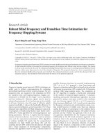
In the second configuration, we turn off the zone-
dependent emissions (so, HMMBD + pde), the resulting
accuracy suffers a 1.5%–2.0% drop as shown in Figures 4 and
5. In the third setting, we use the same setting as the first
setting except that we now use the geometric distribution
that is implicitly incorporated by HMM as the duration
distribution input to the HMMBD (HMMBD + pde + zde
+ Geometric). The purpose is have an approximation of
the performance of the standard HMM with pde and zde
contributions. As show in Figures 4 and 5, the performance

of the result has about 3% to 4% drop (conversely, the
performance improvement with HMMD modeling, with the
duration modeling on the introns in particular, is improved
3%-4% in this case, with a notable robustness at handling
multiple genes in a sequence—as seen in the intron submodel
that includes duration information in [12]). When the
window size becomes 0, that is, when we turn off the setting
EURASIP Journal on Advances in Signal Processing 7
Table 1: Summary of data reduction in C. elegans, Chromosomes I–V.
Summary of data reduction in C. elegans, Chromosomes I–V
File No.ofsequences No.ofalt. %alt. No.ofexons No.ofalt. %alt.
CHROMOSOME I 3537 1306 36.92% 24295 10942 45.04%
CHROMOSOME
II 4161 1316 31.63% 25427 10427 41.01%
CHROMOSOME
III 3277 1220 37.23% 21541 9614 44.63%
CHROMOSOME
IV 3886 1195 30.75% 24390 9509 38.99%
CHROMOSOME
V 5653 1222 21.62% 32135 9122 28.39%
Total 20514 6259 30.51% 127788 49614 38.83%
Table 2: Properties of data set C. elegans, Chromosomes I–V (reduced).
No. of Bases Coding density
Sequences Introns Exons
To t a l B P Av g . L e n . To t a l B P Av g . L e n . To t a l B P Av g . L e n .
67000811 0.24 14255 32547117 2283.2 63919 16371001 256.1 78174 16176057 206.9
0.2
0.3
0.4
0.5

0.6
0.7
0.8
0.9
1
0 2 4 6 8 101214161820
Window size
Accuracy
Exon accuracies
M
= 8
M
= 5
M
= 2
Figure 3: Exon level accuracy rate results with Markov order of 2,
5, and 8, respectively, for C. elegans, Chromosomes I–V.
of position-dependent emissions, the performances of the
results drop sharply as shown in Figures 4 and 5. This is
because the strong information at the transitions, such as
the start codon with ATG or stop codons with TAA, TAG,
or TGA, and so forth, are now “buried” in the bulk statistics
of the exon, intron, or junk regions.
A full fivefold cross validation is performed for the
HMMBD + pde + zde case, as shown in Figures 6 and 7.The
fifth- and second-order Markov models work best, with the
fifth order Markov model having a notably smaller spread in
values consistent with [27] and validating the rapid tuning
performed in Figures 2–5 (that proceeded with analysis using
only one fold). The best case performance was 86% accuracy

at the nucleotide level and 70% accuracy at the base level
0.6
0.7
0.8
0.9
1
0 2 4 6 8 101214161820
Window size
Accuracy
Nucleotide accuracies
HMMBDwithpdeandzde
HMMBD with pde, zde and geo.dist.
HMMBD with pde
Figure 4: Nucleotide level accuracy rate results for three different
kinds of settings.
(compared with 90% on nucleotides and 74% on exons on
the exact same datasets in the meta-HMM described in [27]).
5. Discussion and Conclusions
The gap and hash interpolating Markov models (gIMM and
hIMM) [3] will eventually be incorporated into the model,
since they are already known to extract additional informa-
tion that may prove useful, particularly in the zde regions
where promoters and other gapped motifs might exist.
This is because promoters and transcription factor-binding
sites often have lengthy overall gapped motif structure, and
with the hash-interpolated Markov models, it is possible to
capture the conserved higher order sequence information
in the zde sample space. The hIMM and gIMM methods
will not only strengthen the gene structure recognition, but
also the gene-finding accuracy, and they can also provide

the initial indications of anomalous motif structure in the
regions identified by the gene finder (in a postgenomic phase
of the analysis) [3].
8 EURASIP Journal on Advances in Signal Processing
0
0.1
0.2
0.3
0.4
0.5
0.6
0.7
0.8
0 2 4 6 8 101214161820
Window size
Exon accuracies
Accuracy
HMMBDwithpdeandzde
HMMBD with pde, zde and geo.dist.
HMMBD with pde
Figure 5: Exon level accuracy rate results for three different kinds
of settings.
0
0.2
0.4
0.6
0.8
1
H2 H5 H8
HMMBD performance for 5-fold c.v.

C.Elegans,Chr.I–V,w/oalt-splice
SNSP
AVG
snsp
avg
Figure 6: Nucleotide (red) and exon (blue) accuracy results for
Markov models of order: 2, 5, and 8, using the 5-bin HMMBD
(where the AC value of the five folds is averaged in what is shown).
In this paper we present a novel formulation for inclusion
of side information, beginning with treating the state dura-
tion as side information and thereby bootstrapping from an
HMM to a HMMD modeling capability. We then apply the
method, using binned duration for speedup, HMMBD [10],
to eukaryotic gene-finding analysis and compare to the meta-
HMM [27]. In further work, we plan to merged the methods
to obtain a meta-HMMBD + zde that is projected to have at
least a 3% improvement over the meta-HMM at comparable
time complexity.
0
0.005
0.01
0.015
0.02
H2 H5 H8
HMMBD Std. Dev. for 5-fold c.v.
C.Elegans, Chr. I–V, w/o alt-splice
SNSP
SD
snsp
sd

Figure 7: Nucleotide (red) and exon (blue) standard deviation
results for Markov models of order: 2, 5, and 8, using the 5-bin
HMMBD (where the standard deviation of the AC values of the five
foldsisshown).
Appendices
In Appendix A that follows, we present a description of the
Baum-Welch algorithm in the hidden semi-Markov model
(HSMM) formalism. In Appendix B, we present a descrip-
tion of the Viterbi algorithm in the HSMM formalism.
A. Baum-Welch Algorithm in HMMD
Side-Information Formalism
The Baum-Welch algorithm in the length-martingale side-
information HMMD formalism.
We define the following three variables to simplify what
follows:
s
i
(
d
)
=
⎧
⎪
⎪
⎨
⎪
⎪
⎩
1 − s
i

(
d +1
)
,ifd
= 0,
1
− s
i
(
d +1
)
1 − s
i
(
d
)
· s
i
(
d
)
,if1
≤ d ≤ D − 1,
(A.1)
θ
(
k, i, d
)
= e
i

(
k
)
s
i
(
d
)
,0
≤ d ≤ D − 1,
ε
(
k, i, d
)
= e
i
(
k
)
s
i
(
d
)
,1
≤ d ≤ D − 1.
(A.2)
Define f

t

(i, d) = P(O
1
O
2
···O
t
, S
i
has consecutively
occurred d times up to t
| λ)
f

t
(
i, d
)
=
⎧
⎪
⎪
⎪
⎨
⎪
⎪
⎪
⎩
e
i
(

O
t
)
N

j=1,j
/
= i
F
t−1

j

a
ji
,ifd = 1,
f

t−1
(
i, d
− 1
)
s
i
(
d
− 1
)
e

i
(
O
t
)
,if2
≤ d ≤ D.
(A.3)
EURASIP Journal on Advances in Signal Processing 9
Define
f
t
(
i, d
)
= P
(
O
1
O
2
···O
t
, S
i
ends at t with duration d | λ
)
= f

t

(
i, d
)(
1
− s
i
(
d
))
,1
≤ d ≤ D,
=
⎧
⎨
⎩
θ
(
O
t
, i, d − 1
)
F

t−1
(
i
)
,ifd
= 1,
θ

(
O
t
, i, d − 1
)
f
t−1
(
i, d
− 1
)
,if2≤ d ≤ D,
(A.4)
where
F

t
(
i
)
=
N

j=1,j
/
= i
F
t

j


∗
a
ji
, F
t
(
i
)
=
D

d=1
f

t
(
i, d
)(
1
− s
i
(
d
))
.
(A.5)
Define
b


t
(
i, d
)
= P

O
t
O
t+1
···O
T,
S
i
will have a duration of d from t | λ

=
⎧
⎨
⎩
θ
(
O
t
, i, d − 1
)
B

t+1
(

i
)
,ifd
= 1,
θ
(
O
t
, i, d − 1
)
b

t+1
(
i, d
− 1
)
,if1<d≤ D,
(A.6)
where
B

t
(
i
)
=
N

j=1,j

/
= i
a
ij
B
t

j

, B
t
(
i
)
=
D

d=1
b

t
(
i, d
)
.
(A.7)
Now, f , f
∗
, b and b
∗

can be expressed as
f
∗
t
(
i
)
=
f

t+1
(
i,1
)
e
i
(
O
t+1
)
, b
∗
t
(
i
)
= B
t+1
(
i

)
,
b
t
(
i
)
= B

t+1
(
i
)
, f
t
(
i
)
= F
t
(
i
)
.
(A.8)
Now, define
ω
(
t, i, d
)

= f
t
(
i, d
)
B

t+1
(
i
)
,
μ
t

i, j

= P

O
1
···O
T
, q
t
= S
i
, q
t+1
= S

j
| λ

=
F
t
(
i
)
a
ij
B
t+1

j

,
ϕ

i, j

=
T−1

t=1
μ
t

i, j


,
v
t
(
i
)
= P

O
1
···O
T,
q
t
= S
i
| λ

=
⎧
⎪
⎪
⎪
⎨
⎪
⎪
⎪
⎩
π
(

i
)
B
1
(
i
)
,ift
= 1,
v
t−1
+
N

j=1,j
/
= i

μ
t−1

j, i

− μ
t−1

i, j

,if2≤ t ≤ T.
(A.9)

Using the above equations
π
new
i
=
π
i
b

1
(
i,1
)
P
(
O | λ
)
,
a
new
ij
=
ϕ

i, j


N
j=1
ϕ


i, j

,
e
new
i
(
k
)
=

T
t=1 s.t. O
t
=k
v
t
(
i
)

T
t=1
v
t
(
i
)
,

p
i
(
d
)
=

T
t
=1
ω
(
t, i, d
)

D
d
=1

T
t
=1
ω
(
t, i, d
)
.
(A.10)
B. Viterbi A lgorithm in HMMD
Side-Information Formalism

The Viterbi algorithm in the length-martingale side-
information HMMD formalism.
Define v
t
(i, d) = the most probable path that consecu-
tively occurred d times at state i at time t
v
t
(
i, d
)
=
⎧
⎪
⎪
⎨
⎪
⎪
⎩
e
i
(
O
t
)
N
max
j=1,j
/
= i

V
t−1

j

a
ji
,ifd = 1,
v
t−1
(
i, d
− 1
)
s
i
(
d
− 1
)
e
i
(
O
t
)
,if2
≤ d ≤ D,
(B.1)
where

V
t
(
i
)
=
D
max
d=1
v
t
(
i, d
)(
1
− s
i
(
d
))
. (B.2)
Thegoalistofind
argmax
[
i,d
]

N,D
max
i,d

v
T
(
i, d
)(
1
− s
i
(
d
))

. (B.3)
Define
s
i
(
d
)
=
⎧
⎪
⎪
⎨
⎪
⎪
⎩
1 − s
i
(

d +1
)
,ifd
= 0,
1
− s
i
(
d +1
)
1 − s
i
(
d
)
· s
i
(
d
)
,if1
≤ d ≤ D − 1,
θ
(
k, i, d
)
= s
i
(
d

− 1
)
e
i
(
k
)
,1
≤ d ≤ D,
v

t
(
i, d
)
= v
t
(
i, d
)(
1
− s
i
(
d
))
,1
≤ d ≤ D,
=
⎧

⎪
⎪
⎨
⎪
⎪
⎩
θ
(
O
t
, i, d
)
N
max
j=1,j
/
= i
V
t−1

j

a
ji
,ifd = 1,
v

t−1
(
i, d

− 1
)
θ
(
O
t
, i, d
)
,if2≤ d ≤ D,
(B.4)
where
V
t
(
i
)
=
D
max
d=1
v

t
(
i, d
)
. (B.5)
Thegoalisnow
argmax
[

i,d
]

N,D
max
i,d
v

T
(
i, d
)

. (B.6)
10 EURASIP Journal on Advances in Signal Processing
If we do a logarithm scaling on
s, a and e in advance, the final
Viterbi path can be calculated by:
θ

(
k, i, d
)
= log θ
(
k, i, d
)
= log s
i
(

d
− 1
)
+loge
i
(
k
)
,
1
≤ d ≤ D,
(B.7)
v

t
(
i, d
)
=
⎧
⎪
⎪
⎨
⎪
⎪
⎩
θ

(
O

t
, i, d
)
+
N
max
j=1,j
/
= i

V
t−1

j

+loga
ji

,ifd = 1,
v

t−1
(
i, d
− 1
)
+ θ

(
O

t
, i, d
)
,if2≤ d ≤ D,
(B.8)
where the argmax goal above stays the same.
Acknowledgment
Funding for this research was provided by an NIH K-22
Grant (5K22LM008794, SWH PI).
References
[1] C. Math
´
e, M F. Sagot, T. Schiex, and P. Rouz
´
e, “Current
methods of gene prediction, their strengths and weaknesses,”
Nucleic Acids Research, vol. 30, no. 19, pp. 4103–4117, 2002.
[2] J. D. Ferguson, “Variable duration models for speech,” in
Proceedings of the Symposium on the Application of Hidden
Markov models to Text and Speech, pp. 143–179, 1980.
[3] S. Winters-Hilt, “Hidden Markov model variants and their
application,” BMC Bioinformatics, vol. 7, no. 2, article no. S14,
2006.
[4] P. Ramesh and J. G. Wilpon, “Modeling state durations in
hidden markov models for automatic speech recognition,”
in Proceedings of IEEE International Conference on Acoustics,
Speech and Signal Processing, vol. 1, pp. 381–384, 1992.
[5] S Z. Yu and H. Kobayashi, “An efficient forward-backward
algorithm for an explicit-duration hidden Markov model,”
IEEE Signal Processing Letter s, vol. 10, no. 1, pp. 11–14, 2003.

[6] M. T. Johnson, “Capacity and complexity of HMM duration
modeling techniques,” IEEE Signal Processing Letters, vol. 12,
no. 5, pp. 407–410, 2005.
[7] Z. Ghahramani and M. I. Jordan, “Factorial hidden Markov
models,” Machine Learning, vol. 29, no. 2-3, pp. 245–273,
1997.
[8] S. Fine, Y. Singer, and N. Tishby, “The hierarchical hidden
Markov model: analysis and applications,” Machine Learning,
vol. 32, no. 1, pp. 41–62, 1998.
[9] K. Murphy and M. Paskin, “Linear time inference in hierar-
chical hmms,” in Proceedings of Neural Information Processing
Systems (NIPS ’01), pp. 833–840, December 2001.
[10] S. Winters-Hilt and Z. Jiang, “A hidden markov model with
binned duration algorithm,” IEEE Transactions on Signal
Processing, vol. 58, no. 2, pp. 948–952, 2010.
[11] M. Stanke, R. Steinkamp, S. Waack, and B. Morgenstern,
“AUGUSTUS: a web server for gene finding in eukaryotes,”
Nucleic Acids Research, vol. 32, pp. W309–W312, 2004.
[12] M. Stanke and S. Waack, “Gene prediction with a hidden
Markov model and a new intron submodel,” Bioinformatics,
vol. 19, no. 2, pp. 215–225, 2003.
[13] R. Guig
´
o, P. Agarwal, J. F. Abril, M. Burset, and J. W. Fickett,
“An assessment of gene prediction accuracy in large DNA
sequences,” Genome Research, vol. 10, no. 10, pp. 1631–1642,
2000.
[14] P. A. Stoll and J. Ohya, “Applications of HMM modeling to
recognizing human gestures in image sequences for a man-
machine interface,” in Proceedings of the 4th IEEE International

Workshop on Robot and Human Communication (RO-MAN
’95), pp. 129–134, July 1995.
[15] M. Elmezain, A. Al-Hamadi, J. Appenrodt, and B. Michaelis,
“A hidden markov model-based continuous gesture recogni-
tion system for hand motion trajectory,” in Proceedings of the
19th International Conference on Pattern Recognition (ICPR
’08), December 2008.
[16] J. Appenrodt, M. Elmezain, A. Al-Hamadi, and B. Michaelis,
“A hidden markov model-based isolated and meaningful
hand gesture recognition,” International Journal of Electrical,
Computer, and Systems Engineering, vol. 3, pp. 156–163, 2009.
[17] S. Knerr, E. Augustin, O. Baret, and D. Price, “Hidden Markov
model based word recognition and its application to legal
amount reading on french checks,” Computer Vision and Image
Understanding, vol. 70, no. 3, pp. 404–419, 1998.
[18] M. Schenkel and M. Jabri, “Low resolution, degraded docu-
ment recognition using neural networks and hidden markov
models,” Pattern Recognition Letters, vol. 19, no. 3-4, pp. 365–
371, 1998.
[19] J. Vlontzos and S. Kung, “Hidden markov models for character
recognition,” IEEE Transactions on Image Processing, vol. 1, no.
4, pp. 539–543, 1992.
[20] J. Li, A. Najmi, and R. M. Gray, “Image classification by a
two-dimensional hidden Markov model,” IEEE Transactions
on Signal Processing, vol. 48, no. 2, pp. 517–533, 2000.
[21] J. Li, R. M. Gray, and R. A. Olshen, “Multiresolution image
classification by hierarchical modeling with two-dimensional
hidden Markov models,” IEEE Transactions on Information
Theory, vol. 46, no. 5, pp. 1826–1841, 2000.
[22] C L. Huang, M S. Wu, and S H. Jeng, “Gesture recognition

using the multi-PDM method and hidden Markov model,”
Image and Vision Computing, vol. 18, no. 11, pp. 865–879,
2000.
[23] J. Garcia-Frias, “Hidden markov models for burst error
characterization in indoor radio channels,” IEEE Transactions
on Vehicular Technology, vol. 46, no. 4, pp. 1006–1020, 1997.
[24] E. Bellone, J. P. Hughes, and P. Guttorp, “A hidden Markov
model for downscalling synoptic atmospheric patterns to
precipitation amounts,” Climate Research, vol. 15, no. 1, pp.
1–12, 2000.
[25] C. Raphael, “Automatic segmentation of acoustic musical
signals using hidden Markov models,” IEEE Transactions on
Pattern Analysis and Machine Intelligence, vol. 21, no. 4, pp.
360–370, 1999.
[26] J. A. Kogan and D. Margoliash, “Automated recognition of bird
song elements from continuous recordings using dynamic
time warping and hidden Markov models: a comparative
study,” JournaloftheAcousticalSocietyofAmerica, vol. 103,
no. 4, pp. 2185–2196, 1998.
[27] S. Winters-Hilt and C. Baribault, “A meta-state hmm with
application to gene-structure identification in eukaryotes,”
submitted to EURASIP Genomic Signal Processing.
[28] L. R. Rabiner, “Tutorial on hidden Markov models and
selected applications in speech recognition,” Proceedings of the
IEEE, vol. 77, no. 2, pp. 257–286, 1989.
[29] E. Limpert, W. A. Stahel, and M. Abbt, “Log-normal distribu-
tions across the sciences: keys and clues,” BioScience, vol. 51,
no. 5, pp. 341–352, 2001.
EURASIP Journal on Advances in Signal Processing 11
[30] M. O. Lorenz, “Methods of measuring the concentration of

wealth,” Publications of the American Statistical Association,
vol. 9, no. 70, pp. 209–219, 1905.
[31] A. Krogh, I. S. Mian, and D. Haussler, “A hidden Markov
model that finds genes in E. coli DNA,” Nucleic Acids Research,
vol. 22, no. 22, pp. 4768–4778, 1994.
[32] X. Hong, D. G. Scofield, and M. Lynch, “Intron size, abun-
dance, and distribution within untranslated regions of genes,”
Molecular Biology and Evolution, vol. 23, no. 12, pp. 2392–
2404, 2006.
[33]M.BursetandR.Guig
´
o, “Evaluation of gene structure
prediction programs,” Genomics, vol. 34, no. 3, pp. 353–367,
1996.
[34] “wormbase,” 2009, ttp://www.wormbase.org/.