Báo cáo hóa học: " Research Article High-Resolution Time-Frequency Methods’ Performance Analysis" docx

Hindawi Publishing Corporation
EURASIP Journal on Advances in Signal Processing
Volume 2010, Article ID 806043, 7 pages
doi:10.1155/2010/806043
Research Article
High-Resolution Time-Frequency Methods’ Performance Analysis
Imran Shafi,
1
Jamil Ahmad,
1
Syed Ismail Shah,
1
Ataul Aziz Ikram,
1
Adnan Ahmad Khan,
2
Sajid Bashir,
3
and Faisal Mahmood Kashif
4
1
Information and Computing Department, Iqra University Islamabad Campus, Sector H-9, Islamabad 44000, Pakistan
2
College of Telecommunication Engineering, NUST, Islamabad 44000, Pakistan
3
Computer Engineering Depart ment, Centre for Advanced Studies in Engineering, Islamabad 44000, Pakistan
4
Laboratory for Electromagnetic and Electronic Systems (LEES), MIT Cambridge, Cambridge, MA 02139-4307, USA
Correspondence should be addressed to Imran Shafi, imran.shafi@gmail.com
Received 31 December 2009; Accepted 6 July 2010
Academic Editor: L. F. Chaparro

Copyright © 2010 Imran Shafi et al. This is an open access article distributed under the Creative Commons Attribution License,
which permits unrestricted use, distribution, and reproduction in any medium, provided the original work is properly cited.
This work evaluates the performance of high-resolution quadratic time-frequency distributions (TFDs) including the ones
obtained by the reassignment method, the optimal radially Gaussian kernel method, the t-f autoregressive moving-average spectral
estimation method and the neural network-based method. The approaches are rigorously compared to each other using several
objective measures. Experimental results show that the neural network-based TFDs are better in concentration and resolution
performance based on various examples.
1. Introduction
The nonstationary signals are very common in nature
or are generated synthetically for practical applications
like analysis, filtering, modeling, suppression, cancellation,
equalization, modulation, detection, estimation, coding,
and synchronization. The study of the varying spectral
content of such signals is possible through two-dimensional
functions of TFDs that depict the temporal and spectral
contents simultaneously [1]. Different types of TFDs are
limited in scope due to multiple reasons, for example, low
concentration along the individual components, blurring of
autocomponents, cross terms (CTs) appearance in between
autocomponents, and poor resolution. These shortcomings
result into inaccurate analysis of nonstationary signals.
Half way in this decade, there is an enormous amount
of work towards achieving high concentration along the
individual components and to enhance the ease of iden-
tifying the closely spaced components in the TFDs. The
aim is to correctly interpret the fundamental nature of the
nonstationary signals under analysis in the time-frequency
(TF) domain [2]. There are three open trends that make this
task inherently more complex, that is, (i) concentration and
resolution tradeoff, (ii) application-specific environment,

and (iii) objective assessment of TFDs [1–3]. Tradeoff
between concentration and CTs’ removal is a classical prob-
lem. The concepts of concentration and resolution are used
synonymously in literature whereas for multicomponent
signals this is not necessarily the case, and a difference
is required to be established. High signal concentration is
desired but in the analysis of multicomponent signals reso-
lution is more important. Moreover, different applications
have different preferences and requirements to the TFDs.
In general, the choice of a TFD in a particular situation
depends on many factors such as the relevance of properties
satisfied by TFDs, the computational cost and speed of the
TFD, and the tradeoff in using the TFD. Also selection
of the most suited TFD to analyze the given signal is not
straightforward. Generally the common practice have been
the visual comparison of all plots with the choice of most
appealing one. However, this selection is generally difficult
and subjective.
The estimation of signal information and complexity
in the TF plane is quite challenging. The themes which
inspire new measures for estimation of signal information
and complexity in the TF plane, include the CTs’ suppression,
concentration and resolution of autocomponents, and the
ability to correctly distinguish closely spaced components.
2 EURASIP Journal on Advances in Signal Processing
Efficient concentration and resolution measurement can
provide a quantitative criterion to evaluate performances of
different distributions. They conform closely to the notion of
complexity that is used when visually inspecting TF images
[1, 3].

This paper presents the performance evaluation of high
resolution TFDs that include well-known quadratic TFDs
and other established and proven high resolution and inter-
esting TF techniques like the reassignment method (RAM)
[4], the optimal radially Gaussian kernel method (OKM) [5],
the TF autoregressive moving-average spectral estimation
method (TSE) [6], and the neural network-based method
(NTFD) [7, 8]. The methods are rigorously compared to each
other using several objective measures discussed in literature
complementing the initial results reported in [9].
2. Experimental Results and Discussion
Various objective criteria are used for objective evaluation
that include the ratio of norms-based measures [10], Shan-
non & R
´
enyi entropy measures [11, 12], normalized R
´
enyi
entropy measure [13], Stankovi measure [14], and Boashash
and Sucic performance measures [15]. Both real life and
synthetic signals are considered to validate the experimental
results.
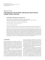
2.1. Bat Echolocation Chirps Signal. The spectrogram of bat
echolocation chirp sound is shown in Figure 1(a), that is
blurred and difficult to interpret. The results are obtained
using the TSE, RAM, OKM, and NTFD, shown in Figure 1.
The TF autoregressive moving-average estimation mod-
els for nonstationary random processes are shown to be a
TF symmetric reformulation of time-varying autoregressive
moving-average models using a Fourier basis [6]. This

reformulation is physically intuitive because it uses time
delays and frequency shifts to model the nonstationary
dynamics of a process. The TSE models are parsimonious
for the practically relevant class of processes with a limited
TF correlation structure. The simulation result depicted in
Figure 1(c) demonstrates that the TSE is able to improve on
the Wigner Distribution (WVD) in terms of resolution and
absence of CTs; on the other hand, the TF localization of the
components deviates slightly from that in the WVD.
The reassignment method enhances the resolution in
time and frequency of the classical spectrogram by assigning
to each data point a new TF coordinate that better reflects
the distribution of energy in the analyzed signal [4]. The
reassigned spectrogram for the bat echolocation chirps signal
is shown in Figure 1(d). The evaluation by various objective
criteria is presented in graphical form at Figure 6 criterions
comparative graphs. The analysis indicates that the results
of the reassignment and the neural network-based methods
are proportionate. However, the NTFD’s performance is
superior based on Ljubisa measure.
On the other hand, the optimal radially Gaussian
kernel TFD method proposes a signal-dependent kernel
that changes shape for each signal to offer improved TF
representation for a large class of signals based on quanti-
tative optimization criteria [5]. The result by this method
is depicted in Figure 1(e) that does not recover all the
components missing useful information about the signal.
Also the objective assessment by various criteria does not
point to much significance in achieving energy concentration
along the individual components.

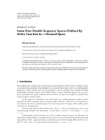
2.2. Synthetic Signals. Four synthetic signals of different
natures are used to identify the best TFD and evaluate their
performance. The first test case consists of two intersecting
sinusoidal frequency modulated (FM) components, given as
x
1
(
n
)
= e
− jπ((5/2)−0.1 sin(2πn/N))n
+ e
jπ((5/2)−0.1 sin(2πn/N))n
. (1)
The spectrogram of the signal is shown in Figure 2(a),
referred to as test image 1 (TI 1).
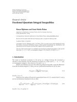
The second synthetic signal contains two sets of nonpar-
allel, nonintersecting chirps, expressed as
x
2
(
n
)
= e
jπ(n/6N)n
+ e
jπ(1+(n/6N))n
+ e
− jπ(n/6N)n
+ e

− jπ(1+(n/6N))n
.
(2)
The spectrogram of the signal is shown in Figure 3(a),
referred to as test image 2 (TI 2).
The third one is a three-component signal containing a
sinusoidal FM component intersecting two crossing chirps,
given as
x
3
(
n
)
= e
jπ((5/2)−0.1 sin(2πn/N))n
+ e
jπ(n/6N)n
+ e
jπ((1/3)−(n/6N))n
.
(3)
The spectrogram of the signal is shown in Figure 4(a),
referred as test image 3 (TI 3). The frequency separation
is low enough and just avoids intersection between the
two components (sinusoidal FM and chirp components) in
between 150–200 Hz near 0.5 sec. This is an ideal signal to
confirm the TFDs’ effectiveness in deblurring closely spaced
components and check its performance at the intersections.
Yet another test case is adopted from Boashash [15]to
compare the TFDs’ performance at the middle of the signal

duration interval by the Boashash’s performance measures.
The authors in [15] have found the modified B distribution
(β
= 0.01) as the best performing TFD for this particular
signal at the middle. The signal is defined as
x
4
(
n
)
= cos

2π

0.15t +0.0004t
2

+cos

2π

0.2t +0.0004t
2

.
(4)
The spectrogram of the signal is shown in Figure 5(a),
referred to as test image 4 (TI 4).
The synthetic test TFDs are processed by the neural
network-based method and the results are shown in Figures

2(b)–5(b), which demonstrate high resolution and good
concentration along the IFs of individual components.
However, instead of relying solely on the visual inspection of
the TF plots, it is mandatory to quantify the quality of TFDs
by the objective methods. The quantitative comparison can
be drawn from Figure 6 (in Figure 6, the abbreviations not
mentioned earlier are the spectrogram (spec), Zhao-Atlas-
Marks distribution (ZAMD), Margenau-Hill distribution
EURASIP Journal on Advances in Signal Processing 3
20
40
60
80
100
120
140
160
Time (s)
50 100 150 200 250 300
Frequency (Hz)
Spectrogram
(a)
20
40
60
80
100
120
140
160

180
Frequency (Hz)
50 100 150 200 250 300 350
NTFD
(b)
TFD obtained by the TSE
(c)
Reassigned spectrogram
(d)
0
25
50
75
100
125
150
175
Time (s)
50 100 150 200 250 300 350 400
Frequency (Hz)
TFD obtained by the OKM
(e)
Figure 1: TFDs of the multicomponent bat echolocation chirp signal by various high resolution t-f methods.
4 EURASIP Journal on Advances in Signal Processing
0
0.5
1
1.5
2
2.5

Time (s)
0 100 200 300 400 500 600 700 800 900
Frequency (Hz)
Test spectrogram TED for synthetic test signal
(a)
0
0.5
1
1.5
2
2.5
Time (s)
0 100 200 300 400 500 600 700 800 900
Frequency (Hz)
Resultant image after processing through NN
(b)
Figure 2: TFDs of a synthetic signal consisting of two sinusoidal FM components intersecting each other. (a) Spectrogram (TI 2) [Hamm,
L
= 90], and (b) NTFD.
0
0.2
0.4
0.6
0.8
1
1.2
Time (s)
0 100 200 300 400 500 600 700 800 900
Frequency (Hz)
Test spectrogram TED for synthetic test signal

(a)
0
0.2
0.4
0.6
0.8
1
1.2
Time (s)
0 100 200 300 400 500 600 700 800 900
Frequency (Hz)
Resultant image after processing through NN
(b)
Figure 3: TFDs of a synthetic signal consisting of two-sets of non-parallel, non-intersecting chirps. (a) Spectrogram (TI 3) [Hamm, L = 90],
and (b) NTFD.
(MHD), and Choi-Williams distribution (CWD)), where
these measures are plotted individually for all the test
images. On scrutinizing these comparative graphs, the NTFD
qualifies the best quality TFD for different measures.
Boashash’s performance measures for concentration
and resolution are computationally expensive because they
require calculations at various time instants. We take a
slice at t
= 64 of the signal and compute the normalized
instantaneous resolution and concentration performance
measures
R
i
(64) and C
n

(64). A TFD that, at a given time
instant, has the largest positive value (close to 1) of the
measure
R
i
is the TFD with the best resolution performance
at that time instant for the signal under consideration. The
NTFD gives the largest value of
R
i
at time t = 64 in Figure 7
and hence is selected as the best performing TFD of this
signal at t
= 64.
On similar lines, we have compared the TFDs’ concentra-
tion performance at the middle of signal duration interval.
EURASIP Journal on Advances in Signal Processing 5
0
0.5
1
1.5
2
2.5
Time (s)
0 100 200 300 400 500 600 700 800 900
Frequency (Hz)
Test spectrogram
(a)
0
0.5

1
1.5
2
2.5
Time (s)
0 100 200 300 400 500 600 700 800 900
Frequency (Hz)
Resultant image after processing through NN
(b)
Figure 4: TFDs of a synthetic signal consisting of crossing chirps and a sinusoidal FM component. (a) Spectrogram (TI 4) [Hamm, L = 90],
and (b) NTFD.
20
40
60
80
100
120
Time (s)
0.05 0.10.15 0.20.25 0.30.35 0.40.45 0.5
Frequency (Hz)
Test spectrogram for closely spaced components
(a)
20
40
60
80
100
120
Time (s)
0.05 0.10.15 0.20.25 0.30.35 0.40.45 0.5

Frequency (Hz)
NNTFD for synthetic signal 4
(b)
Figure 5: TFDs of a signal consisting of two linear FM components with frequencies increasing from 0.15 to 0.25 Hz and 0.2 to 0.3 Hz,
respectively. (a) Spectrogram and (b) NTFD.
A TFD is considered to have the best energy concentration
for a given multicomponent signal if for each signal compo-
nent, it yields the smallest instantaneous bandwidth relative
to component IF (V
i
(t)/f
i
(t)) and the smallest side lobe
magnituderelativetomainlobemagnitude(A
S
(t)/A
M
(t)).
The results plotted in Figure 7 comparative graphs for
Boashash concentration resolution measure indicate that
the NTFD gives the smallest values of
C
1,2
(t)att = 64
and hence is selected as the best concentrated TFD at time
t
= 64.
3. Conclusion
The objective criteria provide a quantitative framework
for TFDs’ goodness instead of relying solely on the visual

measure of goodness of their plots. Experimental results
6 EURASIP Journal on Advances in Signal Processing
10
0
10
1
10
2
10
3
Numerical value of the measure
Spec
WVD
ZAMD
MHD
CWD
TSE
NTFD
RAM
OKM
Type of TFDs
Shannon entropy measure
(a)
6
8
10
12
14
16
18

20
Numerical value of the measure
Spec
WVD
ZAMD
MHD
CWD
TSE
NTFD
RAM
OKM
Type of TFDs
Renyi entropy measure
(b)
6
8
10
12
14
16
18
Numerical value of the measure
Spec
WVD
ZAMD
MHD
CWD
TSE
NTFD
RAM

OKM
Type of TFDs
Volume normalised Renyi entropy measure
(c)
10
−5
10
−4
10
−3
10
−2
Numerical value of the measure
Spec
WVD
ZAMD
MHD
CWD
TSE
NTFD
RAM
OKM
Type of TFDs
Ratio of norm based measure
(d)
10
2
10
3
10

4
10
5
10
6
10
7
Numerical value of the measure
Spec
WVD
ZAMD
MHD
CWD
TSE
NTFD
RAM
OKM
Type of TFDs
Ljubisa measure
TI 1
TI 2
TI 3
TI 4
(e)
Figure 6: Comparison plots, numerical values of criterion versus method employed, for the test images 1–4, (a) The Shannon entropy
measure, (b) R
´
enyi entropy measure, (c) Volume normalized R
´
enyi entropy measure, (d) Ratio of norm based measure, and (e) Ljubisa

measure.
EURASIP Journal on Advances in Signal Processing 7
0
0.1
0.2
0.3
0.4
0.5
0.6
0.7
0.8
0.9
Numerical value of the measure
Spec
WVD
ZAMD
CWD
BJD
Modified B
NTFD
Type of TFDs
Modified Boashash concentration measure (
C
n
)
C1
C3
(a)
0.5
0.55

0.6
0.65
0.7
0.75
0.8
0.85
0.9
0.95
1
Numerical value of the measure
Spec
WVD
ZAMD
CWD
BJD
Modified B
NTFD
Type of TFDs
Boashash normalised instantaneous resolution measure (
R
i
)
(b)
Figure 7: Comparison plots for the Boashash’s TFD performance
measures versus different types of TFDs, (a) The proposed modified
Boashash’s concentration measure (
C
n
(64)), and (b) The Boashash’s
normalized instantaneous resolution measure (

R
i
).
demonstrate the effectiveness of the neural network-based
approach against well-known and established high reso-
lution TF methods including some popular distributions
known for their high CTs suppression and energy concen-
tration in the TF domain.
References
[1] L. Cohen, Time Frequency Analysis, Upper Saddle River, NJ,
USA, 1995.
[2] I. Shafi, J. Ahmad, S. I. Shah, and F. M. Kashif, “Techniques
to obtain good resolution and concentrated time-frequency
distributions: a review,” EURASIP Journal on Advances in
Signal Processing, vol. 2009, Article ID 673539, 43 pages, 2009.
[3] B. Boashash, Time-Frequency Signal Analysis and Processing: A
Comprehensive Reference, Elsevier, Oxford, UK, 2003.
[4] P. Flandrin, F. Auger, and E. Chassande-Mottin, “Time-
frequency reassignment: from principles to algorithms,” in
Applications in Time-Frequency Signal Processing, A. P. Sup-
pappola, Ed., chapter 5, pp. 179–203, CRC Press, Boca Raton,
Fla, USA, 2003.
[5] R. G. Baraniuk and D. L. Jones, “Signal-dependent time-
frequency analysis using a radially Gaussian kernel,” Signal
Processing, vol. 32, no. 3, pp. 263–284, 1993.
[6] M. Jachan, G. Matz, and F. Hlawatsch, “Time-frequency
ARMA models and parameter estimators for underspread
nonstationary random processes,” IEEE Transactions on Sig nal
Processing, vol. 55, no. 9, pp. 4366–4381, 2007.
[7] I. Shafi, J. Ahmad, S. I. Shah, and F. M. Kashif, “Evolutionary

time-frequency distributions using Bayesian regularised neu-
ral network model,” IET Signal Processing,vol.1,no.2,pp.
97–106, 2007.
[8] I. Shafi, J. Ahmad, S. I. Shah, and F. M. Kashif, “Computing
de-blurred time frequency distributions using artificial neural
networks,” in Circuits, Systems, and Signal Processing, vol. 27,
pp. 277–294, Springer, Berlin, Germany; Birkh
¨
auser, Boston,
Mass, USA, 2008.
[9] I. Shafi, J. Ahmad, S. I. Shah, and F. M. Kashif, “Quantitative
evaluation of concentrated time-frequency distributions,” in
Proceedings of the 17th European Signal Processing Conference
(EUSIPCO ’09), pp. 1176–1180, Glasgow, Scotland, August
2009.
[10] D. L. Jones and T. W. Parks, “A resolution comparison of
several time-frequency representations,” IEEE Transactions on
Signal Processing, vol. 40, no. 2, pp. 413–420, 1992.
[11] C. E. Shannon, “A mathematical theory of communication,
part I,” Bell System Technical Journal, vol. 27, pp. 379–423,
1948.
[12] A. R
´
enyi, “On measures of entropy and information,” in
Proceedings of the 4th Berkeley Symposium on Mathematical
Statistics and Probability, vol. 1, pp. 547–561, 1961.
[13] T. H. Sang and W. J. Williams, “Renyi information and
signal-dependent optimal kernel design,” in Proceedings of the
20th International Conference on Acoustics, Speech, and Signal
Processing (ICASSP ’95), vol. 2, pp. 997–1000, Detroit, Mich,

USA, May 1995.
[14] L. Stankovic, “Measure of some time-frequency distributions
concentration,” Signal Processing, vol. 81, no. 3, pp. 621–631,
2001.
[15] B. Boashash and V. Sucic, “Resolution measure criteria for
the objective assessment of the performance of quadratic
time-frequency distributions,” IEEE Transactions on Signal
Processing, vol. 51, no. 5, pp. 1253–1263, 2003.