Báo cáo hóa học: " Research Article A Machine Learning Approach for Locating Acoustic Emission" pdf

Hindawi Publishing Corporation
EURASIP Journal on Advances in Signal Processing
Volume 2010, Article ID 895486, 14 pages
doi:10.1155/2010/895486
Research Article
A Machine Learning Approach for Locating Acoustic Emission
N. F. Ince,
1
Chu-Shu Kao,
2
M. Kaveh,
1
A. Tewfik (EURASIP Member),
1
and J. F. Labuz
2
1
Department of Electrical and Computer Engineering, University of Minnesota, Minneapolis, MN 55455, USA
2
Department of Civil Engineering, University of Minnesota, Minneapolis, MN 55455, USA
Correspondence should be addressed to N. F. Ince, ince
fi
Received 18 January 2010; Revised 26 July 2010; Accepted 20 October 2010
Academic Editor: Jo
˜
ao Marcos A. Rebello
Copyright © 2010 N. F. Ince et al. This is an open access article distributed under the Creative Commons Attribution License,
which permits unrestricted use, distribution, and reproduction in any medium, provided the original work is properly cited.
This paper reports on the feasibility of locating microcracks using multiple-sensor measurements of the acoustic emissions (AEs)
generated by crack inception and propagation. Microcrack localization has obvious application in non-destructive structural
health monitoring. Experimental data was obtained by inducing the cracks in rock specimens during a surface instability test,

which simulates failure near a free surface such as a tunnel wall. Results are presented on the pair-wise event correlation of the AE
waveforms, and these characteristics are used for hierarchical clustering of AEs. By averaging the AE events within each cluster,
“super” AEs with higher signal to noise ratio (SNR) are obtained and used in the second step of the analysis for calculating the
time of arrival information for localization. Several feature extraction methods, including wavelet packets, autoregressive (AR)
parameters, and discrete Fourier transform coefficients, were employed and compared to identify crucial patterns related to P-
waves in time and frequency domains. By using the extracted features, an SVM classifier fused with probabilistic output is used to
recognize the P-wave arrivals in the presence of noise. Results show that the approach has the capability of identifying the location
of AE in noisy environments.
1. Introduction
Rapidly changing environmental conditions and harsh me-
chanical loading are sources of damage to structures. Result-
ing damage can be examined based on local identification
such as the presence of small cracks (microcracks) in a com-
ponent or global identification such as changes in natural
frequency of the structure. Continuous health monitoring
process may involve both global and local identification.
Generally, local damage, such as cracks in critical compo-
nents, is inspected visually. This type of inspection is slow
and prone to human error. Therefore, automated, fast, and
accurate techniques are needed to detect the onset of local
damage in critical components to prevent failure.
In this scheme, nondestructive testing and monitoring
should be employed so that the damage can be inferred
through analysis of the signals obtained from inspection.
Acoustic emission (AE) events can serve as a source of
information for locating the damage, particularly as caused
by the initiation and propagation of microcracks [1–3]. The
spatial distribution of AE locations can provide clues about
the position and extent of the damage [4]. In practice, the
location of AE is estimated from the primary wave (P-wave),

the first part of the signal to arrive at the sensor (see
Figure 2(c)). However, the use of AE waveforms is often
obscured by noise and spurious events, which may cause
misinterpretation of the data. Even in controlled laboratory
settings, it is difficult to account for all the sources of noise.
Therefore, an AE system that automatically “learns” crucial
patterns from the total AE data, as well as particular P-wave
arrivals, may provide clues for distinguishing between real
events and extraneous signals, thus improving the spatial
accuracy of AE locations and reduce false alarms. Accurate
detection of these events with appropriate signal processing
and machine learning techniques may open new possibilities
for monitoring the health of critical components; this offers
the possibility for raising alarms in an automated manner if
the degradation of structural integrity is severe.
In this paper, we describe a novel combination of signal
processing and machine learning techniques based on hier-
archical clustering and support vector machines to process
multi-sensor AE data generated by the inception and prop-
agation of microcracks in rock specimens during a surface
instability test. The effectiveness of the approach is validated
2 EURASIP Journal on Advances in Signal Processing
Preprocessing
(median filter)
AE
Location
estimation
with TOA
SVM-based
P-wave detection

Hierarchical
clustering
Averaging
Envelope detectionFeature extraction
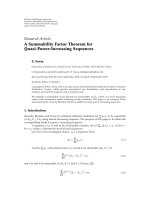
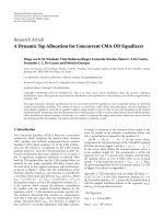
Figure 1: Schematic diagram of the signal processing and classification system. The AE signals were preprocessed with a median filter. In
the following step they are grouped with a hierarchical clustering procedure. An averaging step was implemented in each cluster to improve
the SNR. This is followed by a feature extraction procedure in time and frequency domains. On the test data, the feature extraction and
classification steps were executed when the signal envelope exceeded a predefined threshold. The TOA is calculated by detecting the P-waves
with an SVM classifier.
by laboratory-based experimental results. Fundamental to
the proposed technique is experimentally observed highly
correlated AE waveforms that are generated by the propa-
gation of microcracks [3]. A similar phenomenon was also
reported in [5] by exploring the use of coherence functions
in the frequency domain. Thus, the signal processing frame-
work we present in this study focuses on the capture and
processing of such correlated events as representing signals
of interest for damage localization. The correlated nature
of these events is expected to be different from extraneous
interfering signals within the same measurement bandwidth
that may be generated by other mechanisms with random
characteristics. Several features were extracted from time and
frequency domain using autoregressive modeling, wavelet
packets (WP), and discrete Fourier transform. These features
were used in conjunction with a maximum margin support
vector machine (SVM) classifier coupled with probabilistic
output [6] to recognize the P-waves in the presence of
noise for accurate time of arrival (TOA) calculation. The
classification step is followed by the use of TOA information
of the identified waves of interest for estimating the location

of the microcracks. The feasibility of the proposed techniques
in determining the location of a fracture is presented by
examining AE events recorded by eight sensors attached
to a structure with localized microcracks. A block diagram
summarizing the overall signal processing system is given in
Figure 1.
The remainder of the paper is organized as follows.
In the next section, the experiments and the AE data sets
recorded from two specimens during controlled failure tests
are described. Next, the signal preprocessing techniques used
for enhancing the measured AE signals in the presence of
noise and data acquisition imperfections are presented. This
is followed by a description of a novel hierarchical clustering
technique to group the AE events. The feature extraction
and machine learning techniques for detecting P-waves are
described in Section 4. Finally, the experimental results on
the spatial distributions of AE events are provided and
compared to the actual fracture locations.
2. Acoustic Emission Recordings
AE events were recorded during a surface instability test
that is used to examine failure near a free surface such as
a tunnel wall. A photo representing the experimental setup
(a)
Z
X
Y
(b)
−300
−200
−100

0
100
200
300
Amplitude (mV)
P-wave
0 100 200 300 400 500 600
Samples
(c)
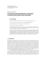
Figure 2: (a) Experimental setup for recording the AE events in
a surface instability test. (b) Coordinate axes of the setup. (c) AE
event recorded from the first sensor that triggers the data acquisition
process. The P-wave is indicated with an arrow; it is the first
component that arrives at the sensor and used for time of arrival
detection.
is given in Figure 2. A prismatic rock specimen, wedged
between two rigid vertical side walls and a rigid vertical rear
wall, is subjected to axial load applied in the Y-direction
through displacing rigid platens. The specimen is supported
in the Z-direction such that compressive stress is generated
passively. The rear wall in X-direction ensures that the lateral
deformation and failure (cracks) were promoted to take place
on the front, exposed face of the specimen.
Four acoustic emission (AE) sensors were attached to the
exposed face using cyanoacrylate glue, and their positions
(x, y, z) were measured. Four other AE sensors were fas-
tened to the side walls of the apparatus. The AE data were
collected with high-speed, CAMAC-based data acquisition
EURASIP Journal on Advances in Signal Processing 3
−10

−5
0
5
10
0 100 200 300 400 500 600 700 800 900 1000
Samples
Normalized amplitude
Original data
(a)
−10
−5
0
5
10
0 100 200 300 400 500 600 700 800 900 1000
Samples
Normalized amplitude
Corrected data
(b)
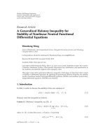
Figure 3: Original signal on (a) corrupted with spikes. At (b), the corrected signal with a median filter.
equipment, consisting of four two-channel modular tran-
sient recorders (LeCroy model 6840) with 8-bit analog to
digital converter (ADC) resolution and a sampling rate of
20 MHz. The data acquisition system was interfaced with
eight piezoelectric transducers (Physical Acoustics model
S9225), and eight preamplifiers with bandpass filters from
0.1 to 1.2 MHz and 40 dB gain were used for conditioning the
raw AE signals. The frequency response of these transducers
ranged from 0.1 to 1 MHz, with a diameter of approximately
3 mm. All channels were triggered when the signal amplitude

exceeded a certain threshold on the first sensor. This sensor
is referred to as the “anchor” sensor. AE data were acquired
in a more or less continuous fashion until 128 Kbytes of
a digitizer memory were filled; then the AE data were
transferred to the host computer, with approximately four
seconds of downtime. The entire waveforms were stored
automatically and sequentially with a time stamp. This
experiment was repeated twice using two very similar rock
specimens with dimensions of 62 mm (X)
× 93 mm (Y) ×
80 mm (Z) labeled as SR1 and SR2. A sample AE signal
recorded with the system is presented in Figure 2(c).Intotal,
2176 and 1536 AE events were recorded in the experiments
SR1 and SR2, respectively. This number includes both real
AE and spurious (noise) events.
Several events contained spikes (Figure 3), which prob-
ably originated from ADC sign errors. Consequently, a
median filter was employed to remove the spikes from the AE
recordings. The median filter is a nonlinear digital filtering
technique that has found widespread application in image
processing. In this study, each sample was replaced with the
median value of a window covering three pre- and post-
samples. A representative corrupted signal and median filter
output is shown in Figure 3. The median filter successfully
corrected the events with consecutive spikes.
3. Clustering of AE Events
In practice, the crack locations are inspected visually by
projecting on a plane the locations of individual AE events,
which are estimated from the TOA information at the
sensors [7]. The TOA is determined by comparing the

signal amplitude to a predefined threshold, where the earliest
arrival is due to the P-wave, as shown in Figures 2 and 4(a).
This type of method produces misleading TOA information
if the signal is noisy, which is usually the case in actual
structures. For instance, the data set we recorded contained
several records with corrupted baseline (Figure 4(b))or
pseudo-AE events. Therefore, before applying the amplitude
threshold, the SNR of the signal was increased by capturing
correlated recordings and averaging grouped events. For
this particular purpose, a hierarchical clustering approach,
which uses the cross-correlation function computed between
different events, was applied.
As a first step, the normalized cross-correlation function
R
xy
[k] was computed for only 256 shifts between pairs of
events represented by the preprocessed signals x[n]andy[n]
acquired at the anchor sensor:
R
xy
[
k
]
=
1
(
N
− k
)
σ

x
σ
y

n
x
[
n
]
y
[
n + k
]
, |k|≤256.
(1)
A correlation matrix was then constructed using the
maximum value of the absolute cross-correlation function
between all event pairs. The lag indices of maximum
correlation between paired events were saved to align the
associated events in further steps of the analysis. The
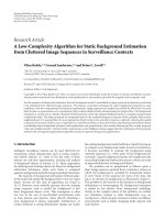
correlation matrices of the two data sets are shown in
Figure 5. These correlation matrices were used to build a
hierarchical cluster [8]. The average linkage method was
used to build the dendrogram, which represented the nested
correlation structure of all AE events. The dendrogram was
cut at level 0.2 in order to cluster those events that have
average cross-correlations equal or larger than 0.8. At this
level, 105 and 80 clusters were obtained with two or more
members for SR1 and SR2, respectively.
AE events related to a particular cluster with four

members are shown in Figure 5.Thisstepwasfollowedby
computing the averages of each cluster to obtain “super”
AE signals. In this scheme, averaging is expected to reduce
the uncorrelated noise in comparison with the repetitive
AE signal component across the records of a given cluster,
resulting in an amplitude SNR increase of at best
√
C,where
C is the number of events in a cluster. A similar approach
has been utilized for processing gene expression profiles in
[9]; it has been shown that averaged gene expression data
within clusters have more predictive power than those from
individual gene expressions. Thus, by increasing the SNR of
the waveforms, AE locations will be more accurate.
4 EURASIP Journal on Advances in Signal Processing
−10
−5
0
5
10
0 500 1000 1500 2000
Samples
Normalized amplitude
(a)
−10
−5
0
5
10
0 500 1000 1500 2000

Samples
Normalized amplitude
(b)
−10
−5
0
5
10
0 500 1000 1500 2000
Samples
Normalized amplitude
(c)
Figure 4: Sample AE recordings. (a) High SNR with clear baseline. (b) Corrupted baseline. (c) Pseudo-AE (noise).
InordertoimprovetheamplitudeSNRbyafactorof
two or more, clusters with at least four members were used
in estimating the location of AE. Those clusters with large
numbers of members increase the reliability of the location
estimation step. We emphasize that the key assumption here,
and one that has been observed experimentally, is the very
low likelihood that, in practice, noise will also be highly
correlated across multiple measurement records. Hence, it
is expected that highly correlated signals (events) can only
originate from a source such as microcracks.
4. P-Wave Detection with SVM
The spatial distribution of AE is estimated from the TOA
information, which is extracted from the waveforms. The
detection of P-waves by a using simple threshold becomes
difficult in the presence of noise or local peaks in the data.
With lower amplitude thresholds, the rate of false positives
(FP) increases rapidly due to the noise in the baseline.

Increasing the amplitude threshold may cause a decrease in
false positive along with the true positive (TP) rate. Con-
sequently, an intelligent algorithm is needed to distinguish
between real and pseudo-P-waves (noise). In this paper, the
use of a maximum margin classifier using input features
extracted from time and frequency domain analysis of the
AE data was investigated for the detection of the P-waves.
In order to determine the TOA accurately, the time and fre-
quency domain properties of the AE data in short windows
around the P-wave arrival were examined. The energy of P-
waves was generally found to be located in lower frequency
bands. This wave was followed by large oscillations with
similar spectral characteristic (the 1st row in Figure 6(a)).
Sample waveforms and spectra related to a typical P-
wave (center frame in the 1st row, Figure 6(a)) and those
windows preceding and following this wave are presented
in frames 1 and 3 in Figure 6(a). The same analysis related
to a segment that may be recognized as a pseudo-P-
wave is also given (Figure 6(b)). It is observed that the
pseudo-P-waves were not followed by large oscillations.
In addition, their frequency spectrum indicates that these
waveforms had a certain amount of energy in mid-frequency
bands. In the following, we describe three approaches
for determining features to be used in a classifier. The
identification of the features was implemented on a training
set by selecting around 20 multichannel “super” AE events
from each data set. The effectiveness of these features and
their combinations are examined on testing datasets in
Section 5.
4.1. Discrete Fourier Transform-Based Features. Based on the

above observations on the frequency characteristics of P-
waves and noise and within the spirit of [10], so-called
Mel Scale, subband energy features were extracted from
the spectrum of each time window using a fast Fourier
transform. A Blackman-Tukey window was used during the
estimation of spectra of segments. In total, five subbands
EURASIP Journal on Advances in Signal Processing 5
2000
1500
1000
500
0
0 500 1000 1500 2000
0.5
0.6
0.7
0.8
0.9
1
Event number
Event number
(a)
1500
1000
500
0
0 500 1000 1500
0.5
0.6
0.7

0.8
0.9
1
Event number
Event number
(b)
Ch-1
Ch-8
100 200 300 400 500 600
Samples
(c)
Figure 5: Correlation matrices of (a) SR1 and (b) SR2. (c) Overlap plot of AE events related to a particular cluster with four members.
were extracted. The widths of the subbands were not uniform
and had a dyadic structure. The lowest two bands had the
same bandwidth, and the following subbands were twice as
wide as the preceding subbands. This setup focused more on
the lower frequency bands since the energy of the signal was
concentrated in this range. By concatenating the Mel Scale
subband features from all three windows, a 15-dimensional
feature vector was constructed. Generally, the noise (pseudo-
P-waves) had jagged spectra. In contrast, the spectra of the
P-waves were smooth. The variance of the derivative of the
spectrum of each time window was also computed as another
feature to capture this difference.
4.2. Discriminatory Wavelet Packet Analysis-Based Features.
In addition to the energies computed in predefined Mel
Scale subbands, we also considered selection of the subbands
adaptively with a discriminant wavelet packet (WP) analysis
technique [11]. In more detail, the signals belonging to
noise and P-waves are decomposed into WP coefficients

over a pyramidal tree structure. In the following step, the
expansion coefficients at each position in the tree structure
are squared and averaged within each class. Then a Euclidean
distance between the averaged expansion coefficients of noise
and P-waves were computed at each node of the WP tree.
The corresponding binary tree structure was pruned from
bottom to top to select the most discriminatory frequency
subbands. This is achieved by comparing the estimated
distance of the children and mother nodes. The energy, in
each selected band, is used as a feature for the recognition
of P-waves. The reader is referred to [11, 12] for a detailed
description of discriminatory wavelet packet analysis and
its derivations. Since short data segments are inspected, we
used a four-tap Daubechies wavelet filter while analyzing
the signals. A tree depth of four was selected, where in
the finest level the available bandwidth was divided in 16
subbands. In Figure 7, we present the selected WP subbands
for the datasets SR1 and SR2, respectively. We note that
the obtained segmentations were somewhat similar in both
datasets. Wider subbands were selected in the left window
preceding the P-wave. We note that the entire high frequency
6 EURASIP Journal on Advances in Signal Processing
024 024
Frequency (MHz)
024
Frequency (MHz) Frequency (MHz)
−20
−10
0
10

log power
Frequency (MHz)
−20
−10
0
10
log power
−20
−10
0
10
20 40 60
Samples
−4
−2
0
2
4
20 40 60
Samples
−4
−2
0
2
4
20 40 60 80 100 120
Samples
Normalized amplitude
−4
−2

0
2
4
(a)
024 024
Frequency (MHz)
024
Frequency (MHz) Frequency (MHz)
−20
−10
0
10
log power
Frequency (MHz)
−20
−10
0
10
log power
−20
−10
0
10
20 40 60
Samples
−4
−2
0
2
4

20 40 60
Samples
−4
−2
0
2
4
20 40 60 80 100 120
Samples
Normalized amplitude
−4
−2
0
2
4
Left Center Right
(b)
Figure 6: (a) Waveforms and log power spectra of 64-sample long time window preceding the P-wave, centered around P-wave, and a 128-
sample long window after the P-wave; (b) Raw data and spectra of noise segments that may be recognized as a pseudo-P-wave.
EURASIP Journal on Advances in Signal Processing 7
01234
L
H
Level
Left Center Right
SR1
(a)
01234
L
H

Level
Left Center Right
SR2
(b)
Figure 7: The WP subband tiling for datasets SR1 (a) and SR2 (b). Each selected subband is weighted with the corresponding log scaled
Euclidean distance between classes. The darker nodes have higher discrimination power.
band was selected as one feature in the left window. The
discriminative power of the high band in the left window
was higher than the high subbands in the center and right
windows, whereas the discriminatory power of the center
and right windows in lower bands were much higher than
the left window. Interestingly, finer levels were selected in the
center and right windows.
4.3. AR Model-Based Features. TheAEdatawerealso
analyzed in the left, center, and right windows using an
autoregressive model. Since the P-waves and oscillations
following them are more structured, it is expected that the
AE waveforms can be well predicted by a linear combination
of the past samples. However, for noise, such a prediction is
expected to fail due to the lack of correlation and/or structure
between consecutive samples. With this motivation, the pre-
diction error of the AR (alternatively the linear predication)
model was used in each time window as another feature for
detecting the P-waves. Prior to employing the AR modeling
in each window, the data were normalized to zero mean and
unit variance in order to eliminate the energy differences
between different events. Since short data segments are
analyzed, the order of the AR model was investigated with
a corrected Akaike information criterion (AICc) of [13],
AIC

=−2log
(
e
)
+2p,
AICc
= AIC +
2p

p +1

N − p −1
,
(2)
where p is the model order, N is the sample size, and e is
the prediction error of the model. The AICc has a second-
order correction for small sample sizes. As the number of
samples gets large, the AICc converges to AIC; therefore,
it can be employed regardless of sample size [13]. In Figure 8,
we present the averaged AICc of both datasets SR1 and SR2
computed in all windows. The AICc criterion indicated a
model order between 6 and 8. To obtain an idea about the
discriminative power of the selected model order, the receiver
operating characteristic (ROC) curves computed on the
training data were also constructed in these three consecutive
time windows for each model order. The area between
the ROC curve (AUC) and the diagonal, no decision,
line was used as a measure to quantify the discrimination
performance of the extracted features. We also inspected
change in discriminatory information as a function of model

order in each analysis window (see Figure 8(b)). However,
the AUC plot suggested lower model orders, where the
model order of p
= 6 provided maximum discriminatory
information.
The ROC curves of different time windows for both
datasets are given in Figure 9. It was observed that the area
under the curve was the maximum in the time window
following the P-wave. This was followed by the window
covering the P-wave. Specifically, the prediction error of the
model was smaller in the last two windows for real P-waves
and provided better discrimination. This is an expected
outcome since the signals in these windows have higher SNR
and are more structured compared to the signals in the first
window.
For each time point, computing the features described
could be a demanding process. To reduce the number of
candidate time points that need to be tested for P-wave
arrival, first the signal was normalized, and then the envelope
of the signal was computed with the Hilbert transform.
When the envelope of the signal exceeded a predefined
threshold, and then that time point was tested for P-wave
8 EURASIP Journal on Advances in Signal Processing
−8
−7
−6
−5
−4
−3
−2

2 4 6 8 10 12
Model order
AICc
(a)
0.34
0.36
0.38
0.4
0.42
0.44
2 4 6 8 10 12
Model order
Area under ROC curve
(b)
Figure 8: (a) The corrected Akaike Information criterion is computed for both datasets SR1 and SR2 and then averaged. The AICc criterion
indicated a model order between 6 and 8, where the minimum was at p
= 8. (b) ROC curve related to prediction error of the AR model on
the training data was computed in the center and right windows and averaged over both datasets SR1 and SR2.
00.20.40.60.81
0
0.2
0.4
0.6
0.8
AUC
= 0.21
Left
1
TP rate
FP rate

(a)
00.20.40.60.81
0
0.2
0.4
0.6
0.8
AUC
= 0.47
Center
SR1
1
TP rate
FP rate
(b)
00.20.40.60.81
0
0.2
0.4
0.6
0.8
AUC
= 0.43
Right
1
TP rate
FP rate
(c)
00.20.40.60.81
0

0.2
0.4
0.6
0.8
AUC
= 0.27
Left
1
TP rate
FP rate
(d)
00.20.40.60.81
0
0.2
0.4
0.6
0.8
AUC
= 0.44
Center
SR2
1
TP rate
FP rate
(e)
00.20.40.60.81
0
0.2
0.4
0.6

0.8
AUC
= 0.39
Right
1
TP rate
FP rate
(f)
Figure 9: The ROC curves related to the model order p = 6 computed on the training data in the left, center, and right windows. Note that
the discrimination in the center and right windows is better than the left window.
EURASIP Journal on Advances in Signal Processing 9
arrival, it was found that a threshold value of 0.5 was
good enough to determine most of the P-waves. The feature
vectors for each method presented above were individually
fed into a linear support vector machine classifier for the
final decision [6]. The main motivation for using an SVM
classifier is based on its robustness against outliers and
its generalization capacity in higher dimensions, which is
the result of its large margin. Furthermore, the output
of the SVM classifier was postprocessed by a sigmoid
function to map the SVM output into probabilities. This
was accomplished by minimizing the cross-entropy error
function as suggested in [14]. By using this procedure, we
were able to assign posterior probabilities to SVM output
which is later used as a confidence level to detect P-
wave arrival. The SVM classifier was trained by selecting
around 20 multichannel “super” AE events from each data
set. Since each event includes AE data from 8 channels,
thisresultedin160P-wavestobetestedineachdataset.
This number included those clusters with low number of

members.However,duetopoorSNR,wewereunableto
visually identify the location of all P-waves in these data
sets. Consequently, we selected those events which have a
visible P-wave. The training feature vectors for P-waves and
noise sets were constructed from this subset by manually
marking the P-wave arrivals and noise events that exceeded
the predefined threshold in each channel. The numbers of
visually identified P-waves were 100 and 78 in datasets SR1
and SR2, respectively. The numbers of noise events were 155
and 162 for SR1 and SR2, respectively. The SVM classifier
was trained on the features using the data set of one of
the experiments and applied it on the other dataset. In this
way, it was guaranteed that no test samples were used in
training the classifier. In addition, using such a training
strategy, it was investigated whether both data sets share
similar patterns. The success of such a strategy can also
validate the generalization capability of the classification
system constructed.
5. Results
As a first step, on each training set, the decision character-
istics of the SVM classifiers were examined by visualizing
the ROC curves related to their outputs. We individually
investigated the ROC curves of each feature extraction
method described above and computed the area between
the diagonal line. In addition, we also considered the
classification performance of SVM when the raw AE data
in these consecutive windows are applied. The ROC curves
related to the training data for SR1 and SR2 are depicted in
Figure 10. We note that the maximum area in both datasets
were obtained with the WP method (0.496 for dataset SR1

and 0.481 for SR2). The second most discriminative features
were Mel scale subband energies obtained with FFT (AUC
=
0.489 and 0.477 for datasets, SR1 and SR2, resp.). On both
datasets, adaptive selection of frequency subbands provided
better performance. We note that the SVMs trained with 256-
dimensional raw AE data had quite poor performance, where
the AUC was 0.39 and 0.31 for datasets SR1 and SR2.
We also examined the performance of a combination
of feature sets. Interestingly, the features computed with
WP method did not provide any better discrimination
performance when they are combined with other features.
For dataset SR1, the best performance was obtained with
those features computed with WP method only. We note
that the best separation performance was obtained with the
combination of Mel Scale, AR model error, and spectrum
variance features on the dataset SR2 (AUC
= 0.483). Based on
these observations, we trained the SVM classifiers either with
only WP features or with the combination of Mel Scale, AR
model error, and spectrum variance features. These classifiers
were applied on the test samples we describe below.
In this study, it is desirable to have a system with low false
positive rates since there exist several peaks in the baseline
preceding the P-waves that can be potentially recognized as a
P-wave. For this particular purpose, we used the probability
output of the SVM classifier. We only accepted those points
as P-Wave arrivals when the posterior probability exceeds a
threshold of 0.9. The threshold can also be moved to more
stringent levels. However, this may result in the classifier

missing the P-waves which will yield low TP rates. One
can also select that time as P-wave arrival point, where the
posterior probability of the SVM classifier is maximum on
the whole AE signal. However, this caused the system to miss
the P-waves and identify those regions in the post-P-wave as
they share similar characteristics. Therefore, we selected the
first point as P-wave when the posterior probability exceeded
the 0.9 threshold.
As indicated in earlier sections, the SVM classifier was
trained on the features using the data set of one of the
experiments and applied on the other dataset. Using this
strategy, we evaluated the generalization capacity of the
system on similar specimens. At this point, it is difficult
to numerically quantify the classification accuracies of both
datasets due to the lack of true labels of the test data. The
true labels can be obtained by manually marking the P-waves.
However, several clusters with low number of members
had poor SNR. It was difficult to visually identify the P-
waves in these records. Consequently, we elected to study
the classification accuracy on those clusters with four or
more members. The algorithm identified 13 and 9 clusters
with four or more members in the datasets SR1 and SR2,
respectively. The super AEs obtained from these clusters had
much higher SNR, and the P-waves were mostly visually
observable. We manually marked the locations of P-waves
and when the classifier identified a region in
±10 samples
around the marked location. We provided such a tolerance
region because the P-wave location was not clearly visible
on small number of records due to low SNR, and the expert

manually marked these positions as possible P-wave location.
The success of the system in recognizing the P-waves with
WP features was 97.1% when SR2 was used as training and
SR1 as testing set. While using SR1 as training and SR2
as testing set, the success on recognizing the P-waves was
94.5%. The combination of features yielded classification
accuracies of 93.3% and 94.5% using the same training
and testing procedure for these datasets, respectively. We
note that similar recognition accuracies were obtained with
10 EURASIP Journal on Advances in Signal Processing
00.20.40.60.81
Mel subbands
AR
Spectrum variance
Wave le t packets
Raw data
0
0.2
0.4
0.6
0.8
1
TP rate
FP rate
(a)
00.20.40.60.81
Mel subbands
AR
Spectrum variance
Wave le t packets

Raw data
0
0.2
0.4
0.6
0.8
1
TP rate
FP rate
(b)
Figure 10: The training classification performance of different feature sets on the dataset SR1 (a) and SR2 (b). The best performance was
obtained with WP approach. The performance of the raw AE data was quite poor compared to other methods.
Ch-1
Ch-8
100 200 300 400 500 600
Samples
Figure 11: Sample cluster average and detected arrivals from eight
sensors of SR1. TOA is marked with a vertical line on each channel.
Note that the SVM classifier was trained on SR2.
both techniques, and the performances were in accordance
with the training data characteristics. Sample TOA estimates
detected by the tuned SVM classifier for a particular cluster
are visualized in Figure 11. The horizontal dashed lines
represent the predefined threshold. Those time points, where
the envelope of the signal exceeded the threshold, were
tested for P-wave arrival. The vertical blue lines represent
the detected P-wave arrivals. Note that, although several
other time points exceeded the threshold, the algorithm
successfully eliminated them. Recall that the SVM classifiers
were trained with different data sets. It was observed that the

SVM classifier successfully recognized the P-waves showing
that the classifier can generalize similar specimens. This may
provide great advantage in the deployment of the system in
real-life applications.
After calculating the arrival information for each sensor,
the iterative algorithm in [15] was used to estimate the
3D hypocenter of the source. For the iterative localization
method, the location errors were described by the symmetric
covariance matrix. The algorithm was executed in a two-step
procedure to improve estimation accuracy. In the first step,
the iterative method computed an optimized AE position
while the covariance matrix that contains spatial variance of
arrival times was examined. The two channels that provided
largest estimated location errors computed from residual
times were disregarded. Then, in the second step, the source
location was estimated with the remaining channels. If no
noticeable reduction was observed, the location estimation
was implemented using all available channels. With this
strategy, we evaluated arrival information from the com-
bination of AE sensors. It should be noted that the AE
location error for the iterative algorithm tested with synthetic
data is generally between 0.5 and 3.0 mm if the P-wave
arrivals can be located within
±10 samples. Figure 12 shows
the estimated locations of all clusters and those with at
least four members. In Figure 13, we present the photos of
EURASIP Journal on Advances in Signal Processing 11
0204060
X-axis
0

10
20
30
40
50
60
70
80
90
0
10
20
30
40
50
60
70
80
90
Y-axisY-axis
0204060
X-axis
(a)
0204060
X-axis
SR1
SR2
0
10
20

30
40
50
60
70
80
90
0
10
20
30
40
50
60
70
80
90
Y-axisY-axis
0204060
X-axis
(b)
0
20
40
60
80
Z-axis
0
20
40

60
0
20
40
60
80
X-axis
Y-axis
Z-axis
0
20
40
60
0
20
40
60
80
X-axis
Y-axis
0
20
40
60
80
(c)
Figure 12: Estimated locations of the AE events for SR1 (first row) and SR2 (bottom row). Each blue circle represents the location of a
particular cluster. The diameter of the circle is proportional to the number of AE in the cluster: (a) The locations of all clusters; (b) the
locations of those clusters with at least four members. Note that the locations are very close to the free surface; (c) the 3D view of the
locations given in the second column.

deformed specimens. The locations were estimated using the
WP features for SR1 and combined feature set for SR2. Note
that the clusters with at least four members have an SNR that
is two times larger than individual recordings. The positions
of the AE sensors were marked with the gray squares. Each
blue circle represents the location of a particular cluster.
The size of each circle is proportional to the number of AE
events within the cluster. The locations of the AE events
were in accordance with the visible crack locations. Most of
the events were localized towards the free surface on both
specimens. Interestingly, the largest clusters were localized a
few millimeters away from the free surface, which matched
well with the observed cracks on the deformed specimens in
both tests (Figures 12(b), 13(a),and13(b)). Several cracks
were developed on or adjacent to the frontal surface in the
X-Y plane in both tests (Figures 13(a) and 13(b)). Especially
for SR2, most clusters were located in the region of X>45,
Y>60, Z<40 mm, which precisely matched with the
heavily cracked zone observed on the Y -Z plane (lower row
in Figures 12(c) and 13(c)).
The locations of all detected clusters in SR1 spread
over the specimen with a tendency towards the free surface
(Figure 12(a)). This is an expected factor since those clusters
with low number of members have lower SNR. It is also
possible to capture noise by chance with a low number of
members. In order to get around this problem, one can
construct another decision system in order to discriminate
between AE and noise. Observations indicate that keeping
12 EURASIP Journal on Advances in Signal Processing
X

Y
X
Y
(a)
0204060
X-axis
SR1
SR2
0
10
20
30
40
50
60
70
80
90
0
10
20
30
40
50
60
70
80
90
Y-axisY-axis
0204060

X-axis
(b)
Z
Y
Z
Y
Y
= 50
Y
= 50
(c)
Figure 13: (a) Photos of the observed cracks at the upper part of the free surface (X = 62 mm). (b) The observed cracks mapped onto X-Y
plane, where the free surface is on the right-hand side (X
= 62 mm). Note that the cracks on SR2 sample are hairline thin. (c) Photos of the
observed cracks on the Z
= 80 mm surface.
those clusters with large number of members automatically
eliminates those recordings with noise or random nature.
One can also increase the correlation threshold for identi-
fying the clusters. However, there is a chance that a high cor-
relation threshold may erase all possible clusters in the data,
where the SNR is low. On the other hand, keeping it very
low relaxes the constraints, where the chance of obtaining
clusters with noise members is increased. The threshold can
be adjusted depending on the quality of the available data.
In order to obtain an idea about the improvement in esti-
mating the location of AE with our technique, we compared
our results to the AE locations estimated using the classic
threshold algorithm. The traditional algorithm uses an
amplitude threshold method to examine P-wave arrivals. The

threshold is determined from the mean signal noise (i.e., pre-
trigger signal) plus/minus 4 times of the standard deviation
or a minimum of
±2 mV. In order to qualify the picked time
mark as a P-wave arrival, two criteria have to be satisfied.
(i) Once the signal exceeds the threshold, it has to sur-
pass the threshold at least 3 times in the subsequent
40-sample (40
× 50 ns = 2 μs) window.
(ii) After 120 samples (i.e., 6 μs) from the picked time
mark, the signal has to exceed threshold at least once.
The threshold method has been studied and proven reli-
able [16] and was chosen due to its simplicity and efficiency
to process thousands of AE events. In Figure 14,wepro-
vide the estimated locations with the traditional threshold
method. We note that the threshold method resulted in a
very scattered pattern of those AE events and did not provide
EURASIP Journal on Advances in Signal Processing 13
0204060
X (mm)
SR1
0
10
20
30
40
50
60
70
80

90
Y (mm)
(a)
02040 60
X (mm)
SR2
0
10
20
30
40
50
60
70
80
90
Y (mm)
(b)
Figure 14: AE locations calculated with classic algorithm on SR1 and SR2 without clustering analysis and SVM technique.
clear information on crack locations. This was due to the
raw AE signals being quite noisy and the TOA that was not
precisely detected by the simple threshold-passing criterion.
The proposed machine learning approach, however, proved
its strength and potential to filter out the noise and enhance
the SNR to correctly identify the position of major cracks.
6. Conclusions
Novel approaches based on hierarchical clustering and sup-
port vector machines (SVM) are introduced for clustering
AE signals and detecting P-waves for microcrack location
in the presence of noise. Prior to feature extraction and

classification process, spikes from the AE data are removed
by employing a median filter. Clusters of AE events are
identified by inspecting their pairwise correlation. After
identifying clusters, an averaging step was implemented
to obtain “super” AE with improved SNR. Characteristic
features were extracted from the data in time and frequency
domains to identify P-waves for time of arrival (TOA). SVM
classifiers with probabilistic outputs were trained with these
features to recognize P-waves for TOA determination. The
location of each AE cluster was estimated accordingly.
The proposed machine learning technique with cluster-
ing analysis and SVM showed that the estimated clusters
can successfully indicate the location of failure observed in
surface instability tests, in which the cracks were promoted
to occur close to the front free surface of the specimen. This
approach, compared to the classic AE algorithm that gave a
very disperse pattern and was not indicative of the region of
failure, also presents the capability of filtering noisy signals
and enhance the SNR to obtain more reliable AE cluster
locations. The preliminary results show that the method
has the potential to be a component of a structural health
monitoring system.
Acknowledgments
Partial support was provided by the National Science Foun-
dation, Grant no.CMMI-0825454. The authors express their
appreciation for the constructive comments provided by the
referees, which served to considerably improve the paper.
References
[1]C.Grosse,S.D.Glaser,andM.Kr
¨

uger, “Wireless acoustic
emission sensor networks for structural health monitoring in
civil engineering,” in Proceedings of the European Conference
on Non-Destructive Testing (ECNDT ’06), pp. 1–8, Berlin,
Germany, 2006.
[2] L. Golaski, P. Gebski, and K. Ono, “Diagnostics of reinforced
concrete bridges by acoustic emission,” Journal of Acoustic
Emission, vol. 20, pp. 83–98, 2002.
[3] V.Emamian,M.Kaveh,A.H.Tewfik,Z.Shi,L.J.Jacobs,and
J. Jarzynski, “Robust clustering of acoustic emission signals
using neural networks and signal subspace projections,”
EURASIPJournal on Applied Signal Processing, vol. 2003, no.
3, pp. 276–286, 2003.
[4] Z. Gong, E. O. Nyborg, and G. Oommen, “Acoustic emission
monitoring of steel railroad bridges,” Materials Evaluation,
vol. 50, no. 7, pp. 883–887, 1992.
[5] C. U. Grosse, F. Finck, J. H. Kurz, and H. W. Reinhardt,
“Improvements of AE technique using wavelet algorithms,
coherence functions and automatic data analysis,” Journal of
Construction and Building Mater ials, vol. 18, no. 3, pp. 203–
213, 2004.
[6] T. Hastie, R. Tibshirani, and J. Friedman, The Elements of
Statistical Learning, Springer, New York, NY, USA, 2001.
[7] N. Iverson, C S. Kao, and J. F. Labuz, “Clustering analysis of
AE in rock,” Journal of Acoustic Emission, vol. 25, pp. 364–372,
2007.
[8] S. Theodoridis and K. Koutroumbas, Pattern Recognition
Second Edition, Academic Press, New York, NY, USA, 2003.
14 EURASIP Journal on Advances in Signal Processing
[9] M. Y. Park, T. Hastie, and R. Tibshirani, “Averaged gene

expressions for regression,” Biostatistics, vol. 8, no. 2, pp. 212–
227, 2007.
[10] A. E. Cetin, T. C. Pearson, and A. H. Tewfik, “Classification
of closed and open shell pistachio nuts using principal
component analysis of impact acoustics,” in Proceedings of the
IEEE International Conference on Acoustics, Speech, and Signal
Processing (ICASSP ’04), pp. 677–680, May 2004.
[11] N. Saito, Local feature extraction and its applications using a
library of bases, Ph.D. thesis, Department of Mathematics, Yale
University, New Haven, Connm USA, December 1994.
[12] N. F. Ince, F. Goksu, A. H Tewfik, I. Onaran, A. E. Cetin, and
T. Pearson, “Discrimination between closed and open-shell
(Turkish) pistachio nuts using undecimated wavelet packet
transform,” Biological Eng i neering Journal, American Society of
Agricultural and Biolog ical Engineers (ASABE),vol.1,no.2,pp.
159–172, 2008.
[13] K. P. Burnham and D. R. Anderson, Model Selection and Mul-
timodel Inference: A Practical Information-Theoretic Approach,
Springer, New York, NY, USA, 2nd edition, 2002.
[14] J. C. Platt, “Probabilistic outputs for support vector machines
and comparisons to regularized likelihood,” in Advances in
Large Margin Classifiers, A. Smola, P. Bartlett, B. Sch
¨
olkopf,
and D. Schuurmans, Eds., MIT Press, Cambridge, Mass, USA,
1999.
[15] J.H. Kruz, S. Koppel, L. Linzer, B. Schechinger, and C. U.
Grosse, “Source localization,” in Acoustic Emission Testing:
Basics for Research-Applications in Civil Engineering,C.U.
Grosse and M. Ohtsu, Eds., chapter 6, Springer, Berlin,

Germany, 2008.
[16] K. R. Shah and J. F. Labuz, “Damage mechanisms in stressed
rock from acoustic emission,” Journal of Geophysical Research,
vol. 100, no. 8, pp. 15527–15539, 1995.