Báo cáo hóa học: " Research Article Video Frames Reconstruction Based on Time-Frequency Analysis and Hermite Projection Method" docx
Bạn đang xem bản rút gọn của tài liệu. Xem và tải ngay bản đầy đủ của tài liệu tại đây (7.1 MB, 11 trang )
Hindawi Publishing Corporation
EURASIP Journal on Advances in Signal Processing
Volume 2010, Article ID 970105, 11 pages
doi:10.1155/2010/970105
Research Article
Video Frames Reconstruction Based on Time-Frequency
Analysis and Hermite Projection Me thod
Srdjan Stankovi
´
c,
1
Irena Orovi
´
c,
1
and Andrey Krylov
2
1
Faculty of Electrical Engineering, University of Montenegro, 20000 Podgorica, Montenegro
2
Faculty of Computational Mathematics and Cybernetics, Lomonosov Moscow State University, Moscow119991, Russia
Correspondence should be addressed to Irena Orovi
´
c,
Received 15 February 2010; Revised 3 July 2010; Accepted 14 August 2010
Academic Editor: Sridhar Krishnan
Copyright © 2010 Srdjan Stankovi
´
c et al. This is an open access article distributed under the Creative Commons Attribution
License, which permits unrestricted use, distribution, and reproduction in any medium, provided the original work is properly
cited.
A method for temporal analysis and reconstruction of video sequences based on the time-frequency analysis and Hermite
projection method is proposed. The S-method-based time-frequency distribution is used to characterize stationarity within
the sequence. Namely, a sequence of DCT coefficients along the time axes is used to create a frequency-modulated signal. The
reconstruction of nonstationary sequences is done using the Hermite expansion coefficients. Here, a small number of Hermite
coefficients can be used, which may provide significant savings for some video-based applications. The results are illustrated with
video examples.
1. Introduction
Video signal exchange and storage are very important in
multimedia applications. For this purpose, different kinds
of video processing techniques are needed, such as video
compression algorithms, video denoising methods, and
scene analysis [1–4]. Depending on the video quality and
bit-rate constraints, various compression algorithms have
been developed [5–10]. These algorithms commonly employ
motion-compensated differential coding (known as P and
B frames), that is the interframe prediction based on the
reference frames (I-frames). I-frames are set at user-defined
intervals (e.g., 1 key frame for every 5 frames, or 15 frames,
etc.). Thus, the algorithm compares two images and sends
only the parts of the following images (B- and P-frames)
that differ from the reference image [5]. For example,
such algorithms are MPEG-2 compression and its improved
version MPEG-4 [6]. A good implementation of MPEG-
4 can additionally reduce the bit rate for approximately
15%, but it requires high processing power. Furthermore,
the H.264 standard improves compression in comparison
to MPEG-4 [6–8]. It offers many additional but optional
tools, so that the compression ratio will significantly vary
for different implementations. The most popular Baseline
Profile provides a bit rate reduction of 10%
−30% over
MPEG-4, but it requires almost twice the CPU power. An
overly simple H.264 implementation may produce worse
results than an MPEG-4 implementation while the Main
Profile is computationally heavy. Finally, some applications
use the Moving-JPEG (MJPEG) multimedia format, where
video frames are separately compressed as JPEG images [9].
It does not include interframe prediction, which results in
lower compression ratio. However, it has been commonly
used by digital still cameras for the unified treatment of still
and video compression. Also, it has been used for IP-based
video cameras via HTTP streams.
Here, we propose a method for video sequence recon-
struction based on the time-frequency analysis and Hermite
projections. The main goal of this paper is not to provide
a specific compression solution for video applications,
but rather an auxiliary tool for other video processing
algorithms, such as video surveillance, motion tracking, and
video compression. Combined with the existing compres-
sion algorithms, this approach can additionally reduce the
amount of data required for high-quality video reconstruc-
tion. It does not use the exhaustive search procedures for
motion estimation, spatial or temporal prediction, or the
computationally demanding advanced options included in
2 EURASIP Journal on Advances in Signal Processing
other approaches. The proposed procedure can be applied
to the coefficients of raw video format or the reference
frames (I frames) of coded video, or to the coefficients within
the sequence of JPEG images. Therefore, the possibility to
merge it with the existing techniques could be interesting for
researchers and could provide additional improvements of
compression ratio.
The procedure consists of two parts. The first one
employs the time-frequency analysis to examine the tem-
poral stationarity/non-stationarity of the coefficients over
time. When observing a sequence of video frames, one may
distinguish between stationary scene regions that do not
change over time and dynamic scene regions containing
moving objects (nonstationary regions). Video sequences
usually contain noise, causing coefficients to vary, even in
the absence of moving objects. In order to reduce the noise
influence, here we propose a time-frequency-based proce-
dure for temporally stationary and nonstationary coefficients
characterization. Various time-frequency distributions have
been used for the analysis of noisy nonstationary signals
with different instantaneous frequency laws [11, 12]. Here,
we focus on the use of computationally efficient quadratic
distribution called the S-method [13, 14]. To characterize
temporal behaviour, the sequence of coefficients at the
position (x, y) is analyzed by using the S-method.
The second part of the proposed procedure deals with
the high-quality reconstruction of the coefficients. The
reconstruction of a stationary sequence is based on its first
coefficient. On the other hand, the efficient reconstruction
of nonstationary sequences of coefficients is obtained by
using the Hermite projection method [15]. Namely, by using
a certain number of Hermite coefficients, nonstationary
sequence can be reconstructed. This number could be quite
smaller than the length of original sequence. Although, the
quality of reconstructed video depends on the number of
Hermite functions, significant savings can be achieved even
if a high video quality is required.
The paper is organized as follows. Section 2 describes the
theory behind the time-frequency analysis and its application
for characterizing the temporal stationarity. In Section 3, the
reconstruction procedure based on the Hermite projection
method is proposed. In Section 4, the proposed method is
applied to the examples. Concluding remarks are given in
Section 5.
2. Theoretical Background
A brief theoretical background on the S-method-based time-
frequency analysis and the Hermite projection method is
presented in this Section. The time-frequency analysis will
be used to characterize the stationarity of video coefficients
over time while the Hermite projection method reduces the
amount of data for high-quality video reconstruction.
2.1. Time-Frequency Analysis—the S-Method. Time-freque-
ncy representations have been used to analyze the time-
varying spectral properties of nonstationary signals. The
commonly used approaches are obtained by introducing
the time dependency into the Fourier analysis using the
time-windowing technique. Hence, the short time Fourier
transform (STFT) is defined as follows [12]:
STFT
(
t, ω
)
=
∞
−∞
x
(
t + τ
)
w
(
τ
)
e
−jωτ
dτ,(1)
where x(t)isasignal,andw(t) is a window function. The
spectrogram is the energetic version of STFT and it is defined
as SPEC(t, ω)
=|STFT(t, ω)|
2
. The main drawback of
the spectrogram is a low time-frequency resolution. There-
fore, the quadratic distributions are introduced to improve
time-frequency concentration. An efficient quadratic time-
frequency distribution is obtained by the S-method. It is
defined as follows [13]:
SM
(
t, ω
)
=
∞
−∞
P
(
θ
)
STFT
(
t, ω + θ
)
STFT
∗
(
t, ω
−θ
)
dθ,
(2)
where P(θ) is a finite frequency domain window. The S-
method preserves the autocomponents concentration as
in the Wigner distribution but significantly reduces or
removes the cross-terms. Unlike the Wigner distribution, the
oversampling in time domain is not necessary because the
aliasing components will be removed in the same way as
the cross-terms. The discrete form of the S-method can be
written as follows:
SM
(
n, k
)
=
L
l=−L
P
(
l
)
STFT
(
n, k + l
)
STFT
∗
(
n, k
−l
)
=|STFT(n, k)|
2
+2Real
⎧
⎨
⎩
L
l=1
STFT
(
n, k + l
)
STFT
∗
(
n, k
−l
)
⎫
⎬
⎭
,
(3)
where n and k denote discrete time and frequency, respec-
tively, while the rectangular window P(l) is assumed. Param-
eter L determines the frequency window width which is
2L + 1. Windowing the product in the convolution through
the narrow window P(l), the cross-terms will be reduced or
even removed. Thus, by choosing an appropriate value of L,
the sharpness of the Wigner distribution can be preserved
while avoiding the cross-terms. Namely, high autoterms
concentration is obtained with only a few summation terms
due to the fast convergence within P(l). Hence, in many
practical applications L<5 is a suitable choice (e.g., L
= 3).
Also, as shown in the sequel, a lower L value requires a fewer
number of computations.
The S-method is computationally less demanding in
comparison with other quadratic distributions. It requires
N(3 + L)/2 complex multiplications and N(6 +L)/2complex
additions (N is the number of samples within the window),
unlike the Wigner distribution which requires N(4+log
2
N)/2
complex multiplications and Nlog
2
2N complex additions.
Also, the S-method allows simple and efficient hardware
realization that has already been done [14].
EURASIP Journal on Advances in Signal Processing 3
2.2. Fast Hermite Projection Method. The Hermite projection
method has been introduced in various image and speech
processing applications [15–19]. Namely, it has been shown
that this method could be efficient in image database
retrieval, image filtering, texture analysis, text-independent
speaker indentification, and so forth. The expansion into
Hermite functions provides good localization in both signal
and transform domain. Although the computation of Her-
mite functions seems to be a demanding task, they could be
easily obtained using recursive realization as follows:
Ψ
0
(
x
)
=
1
4
√
π
e
−x
2
/2
,
Ψ
1
(
x
)
=
√
2x
4
√
π
e
−x
2
/2
,
Ψ
p
(
x
)
= x
2
p
Ψ
p−1
(
x
)
−
p −1
p
Ψ
p−2
(
x
)
,
∀p ≥ 2.
(4)
The first step in the Hermite projection method is to remove
the baseline since:
ψ
p
(
x
)
−→ 0, |x|−→∞. (5)
The baseline is defined as follows:
b
x
y
=
F
(
x,0
)
+
F
(
x, P
)
−F
(
x,0
)
P
· y,(6)
where F(x, y) is a two-dimensional signal, x
= 0, , P and
y
= 1, , Q, while the baseline is b(x, y) = b
x
(y)forafixed
x. Further, the baseline is subtracted from the original values
as follows:
f
x, y
= F
x, y
−b
x, y
. (7)
The decomposition into N Hermite functions is defined as:
f
y
(
x
)
=
N−1
p=0
c
p
ψ
p
(
x
)
,(8)
where f
y
(x) = f (x, y)holdsforafixedy, while the
coefficients of Hermite expansion are
c
p
(
x
)
=
∞
−∞
f
y
(
x
)
ψ
p
(
x
)
dx. (9)
Fast Hermite projection method uses the Gauss-Hermite
quadrature to calculate the Hermite expansion coefficients as
follows [15, 16]:
c
p
(
x
)
≈
1
M
M
m=1
μ
p
M
−1
(
x
m
)
f
(
x
m
)
, (10)
where x
m
are zeros of Hermite polynomials
H
p
(
x
)
=
(
−1
)
p
e
x
2
d
p
e
−x
2
dx
p
. (11)
The constants μ
p
M
−1
(x
m
) are obtained using the Hermite
functionsasfollows:
μ
p
M
−1
(
x
m
)
=
ψ
p
(
x
m
)
ψ
M−1
(
x
m
)
2
. (12)
1
31
61
91
121 151
181 211
241
271
301 331
1
1
1
1
1
1
1
1
1
1
1
1
2
2
2
2
2
2
2
2
2
2
2
2
Figure 1: An illustration of stationary and nonstationary blocks in
a sequence of frames (box 1-stationary block, box 2-nonstationary
block).
3. Video Analysis and Reconstr uction Using
Time-Frequency Representations and Fast
Hermite Projection Method
3.1. Analysis of Temporal Stationarity within the Video
Sequence. By observing a video scene over time, usually
there are some blocks that do not change (the box marked
by 1 in Figure 1) while the others vary, for example, due
to the presence of moving objects (the box marked by 2
in Figure 1).Thesetwotypesofblockswillbereferred
to as stationary and nonstationary blocks, respectively. For
example, a temporal sequence of pixels belonging to the
stationary block should represent a constant amplitude sig-
nal, unlike the sequence of pixels from nonstationary block.
Thesameholdswhenasequenceoffrequencycoefficients,
for example Discrete Cosine Transform (DCT) coefficients,
is observed instead of pixels. Thus, in order to analyze the
stationarity/non-stationarity within the sequence of frames,
a procedure described in the sequel can be applied to
different coefficients. We focus on the DCT coefficients, since
they are usually employed in image and video processing
algorithms.
The video frames are split in 8
× 8 blocks and DCT
coefficients are calculated. Further, the sequence of DC
coefficients within the K consecutiveframesisconsideredas
follows:
DC
n
1
,n
2
(
t
)
=
DC
n
1
,n
2
(
t
1
)
,DC
n
1
,n
2
(
t
2
)
, ,DC
n
1
,n
2
(
t
K
)
,
(13)
where block position (n
1
, n
2
) is determined by the position
of its first coefficient while t
1
, t
2
, ,t
K
indicate frames’
numbers.
4 EURASIP Journal on Advances in Signal Processing
200 400 600 800 1000 1200
Time (frames)
DC AC (1, 2) AC (2, 1)
60
50
40
30
20
10
Frequency
60
50
40
30
20
10
Frequency
60
50
40
30
20
10
Frequency
60
50
40
30
20
10
Frequency
200 400 600 800 1000 1200
Time (frames)
200 400 600 800 1000 1200
Time (frames)
(a)
200 400 600 800 1000 1200
Time (frames)
DC AC (1, 2) AC (2, 1)
60
50
40
30
20
10
Frequency
60
50
40
30
20
10
Frequency
60
50
40
30
20
10
Frequency
60
50
40
30
20
10
Frequency
200 400 600 800 1000 1200
Time (frames)
200 400 600 800 1000 1200
Time (frames)
(b)
Figure 2: Time-frequency representations of coefficients belonging to: (a) nonstationary block, (b) stationary block.
Thetemporalsequenceofcoefficients may contain the
nonstationarities due to the motion, noise, or luminance
variations. Thus, the stationary sequence becomes slightly
nonstationary even in the presence of a small amount of
noise. The comparison between consecutive coefficients may
lead to an incorrect conclusion. Consequently, DC
n
1
,n
2
(t) −
DC
n
1
,n
2
(t) cannot be used to indicate whether a sequence
is stationary or not. In order to eliminate the influence of
noise, the time-frequency analysis is employed. Therefore,
the examination of stationarity is performed by using the
time-frequency-based instantaneous frequency estimation. It
is estimated as a position of the time-frequency distribution
maxima as explained below.
Based on DC
n
1
,n
2
(t), a frequency-modulated signal x(t)is
created as follows [17]:
x
n
1
,n
2
(
t
)
= e
jμ(DC
n
1
,n
2
(t)−DC
n
1
,n
2
(t))·t
, (14)
where
DC
n
1
,n
2
= mean(DC
n
1
,n
2
) while μ is a constant that
controls time-frequency resolution and t is a time vector.
Thus, for each 8
× 8block,64frequency-modulated
signals are created. Further, for the signal x
n
1
,n
2
(t), the time-
frequency distribution is obtained by using the S-method as
follows:
SM
x
(
t, ω
)
=
L
i=−L
P
(
i
)
STFT
x
(
t, ω + i
)
STFT
x
∗
(
t, ω
−i
)
.
(15)
One may note that
ω = arg max{SM
x
(
t, ω
)
}=μ
DC
n
1
,n
2
(
t
)
−DC
n
1
,n
2
(
t
)
.
(16)
Therefore, if
ω = const, the block at the position (n1, n2)
is stationary and will remain unaltered within K consecutive
frames. Otherwise, the observed block is nonstationary.
The AC components (the alternating components, that
is, the remaining 63 components in the 8
× 8 DCT block)
within the stationary block are stationary as well. The
AC components within the nonstationary block should be
analyzed separately. The S-method of a sequence of DC
components belonging to nonstationary and stationary 8
×8
blockaregiveninFigures2(a) and 2(b), respectively. Also,
time-frequency representations of two AC components are
included.
The time-frequency representation of stationary
sequence should be robust to certain amount of noise,
meaning that it should be flat even in the presence of noise.
Otherwise, the nonstationarities caused by the noise may
be interpreted as nonstationarities due to the motion. Note
that additive noise within the sequence DC
n
1
,n
2
(t)becomes
multiplicative one after the frequency-modulated signal
is formed (according to (14)). The performance of time-
frequency distributions in the presence of multiplicative
noises has been studied in the literature [20–23], where
various analyses and optimality conditions have been
derived. Here, numerous experiments have been performed
to prove good characteristics of the proposed approach in a
noisy environment.
It has been shown, (in Figure 3), that the proposed
method can be robust in the presence of some additional
Gaussian (zero mean and variance up to 0.001) and impulse
noise (noise density up to 0.002) added to the video frames.
In particular, three cases are observed for a stationary
sequence:
EURASIP Journal on Advances in Signal Processing 5
(i) Figure 3(a)—no additional noise (just the noise
caused by luminance variations),
(ii) Figure 3(b)—with Gaussian noise,
(iii) Figure 3(c)—with impulse noise.
In each case, one sample frame is illustrated (left), as well as
the noisy sequence of DC coefficients and its time-frequency
representation (right), which is flat even in the presence of
noise.
In order to speed up the procedure, the S-method can be
calculated for several components at the same time. Namely,
a frequency-modulated signal x(t) can be modified into
multicomponent signal as follows:
x
M
(
t
)
=
M−1
q=0
x
q
(
t
)
,
x
0
(
t
)
= e
jμ(DC
n
1
,n
2
(t)−DC
n
1
,n
2
(t)) ·t−jβ
0
t,
x
q
(
t
)
= e
jμ(AC
q
n
1
,n
2
(t)−AC
q
n
1
,n
2
(t)) ·t−jβ
q
t
,
q>0,
(17)
where AC
q
is an AC component within the 8 × 8 block.
The S-method provides a cross-term free representation,
but the components have to be spaced from each other by
using the constants β0, , βq. Namely, these constants are
used to shift the components up and down from the central
frequency, so that they do not overlap. They are integers
whose values depend on the window width and can be
chosen experimentally.
3.2. Hermite Projection-Based Temporal Reconstruction of
Nonstationary Pixels within the Sequence of Video Frames.
The Hermite functions are used as the basis functions
for the video sequence expansion method due to their
favorable properties. They represent an independent set
of orthogonal functions, with good localization. Therefore,
they can provide a unique representation of signals, while
the coefficients of expansion are easily computed. Hence,
the Hermite functions-based transform has been used in
many applications for different types of signals, especially for
images [15, 16]. Beside the Hermite functions, some other
possible basis functions with desirable properties are Leg-
endre polynomial, Laguerre polynomials, Bessel functions,
and so forth [18]. For instance, the Legendre polynomials
are defined on normalized intervals [
−1, 1] and their Fourier
transform has infinite spread. Thus, there are difficulties
to determine the expansion coefficients when the original
signal is not explicitly given. The uncertainty inequalities for
Laguerre polynomials cannot be easily reduced to a form
that involves only expansion coefficients. In the case of Bessel
function, the derivation of the coefficients from explicit or
implicit information about the signal is very complicated
[18].
Furthermore, by using the Hermite expansion, the signal
energy is approximated by the numerical integral of the
Gauss-Hermite type and converges more rapidly than the
−40
−20
0
20
Sequence of DC coefficients
60 120
Time (frames)
40
30
Frequency
20
10
60 120
(a)
−40
−20
0
20
Sequence of DC coefficients
60 120
Time (frames)
40
30
Frequency
20
10
60 120
(b)
−40
−20
0
20
Sequence of DC coefficients
60 120
Time (frames)
40
30
Frequency
20
10
60 120
(c)
Figure 3: (a) without additional noise, (b) with Gaussian noise
(zero mean and variance 0.001), (c) with impulse noise (noise
density 0.002).
rectangle rule in the case of the DCT [19]. Therefore, the
Hermite functions allow for a higher concentration of signal
energy at lower frequencies and lead to better compression.
Consider the pixels (n1, n2), whose intensity varies over
time. For K frames, we can observe a nonstationary sequence
in the following form:
V
=
p
n
1
,n
2
(
1
)
, p
n
1
,n
2
(
2
)
, p
n
1
,n
2
(
3
)
, , p
n
1
,n
2
(
K
)
, (18)
where p
n1,n2
(k) represents a pixel value in the kth frame. The
sequence V(t) can be decomposed into N Hermite functions:
6 EURASIP Journal on Advances in Signal Processing
V
≈
N−1
p
=0
c
p
ψ
p
(x). AsequenceofK elements can be
reconstructed even by a small number of Hermite coefficients
c
p
, that is, for N<K.An error, depending on the value of
N, is introduced by the reconstruction. Thus, with a suitable
choice of N, a sequence with K pixels can be represented
using smaller number (N)ofcoefficients without significant
quality degradation.
Instead of pixels, one can reconstruct DCT coefficients
within the 8
× 8 blocks. For instance, a temporal sequence
of DC components from the 8
×8 blocks whose central pixels
are on the (n1, n2) position is
V
DC
=
DC
n
1
,n
2
(
1
)
,DC
n
1
,n
2
(
2
)
,DC
n
1
,n
2
(
3
)
, ,DC
n
1
,n
2
(
K
)
.
(19)
The original nonstationary sequence V
DC
for K = 360
videoframesisillustratedinFigure 4(a). Its time-frequency
representation is given in Figure 2(a) (frames from 224 to
584). The two reconstructed sequences with N
= 240 and
N
= 180 Hermite coefficients are illustrated in Figures
4(b) and 4(c), respectively. An additional moving average
smoothing procedure is applied as well
DC
N
(
k
)
=
DC
N
(
k
−1
)
+DC
N
(
k +1
)
2
, (20)
where DC
N
(k) denotes the kth element of sequence recon-
structed by N Hermite coefficients. Namely, the moving
average smoothing is used to reduce the errors introduced by
the reconstruction when the number of Hermite coefficients
is significantly lower than the number of the original
coefficients, such as K/N
= 180/360 = 1/2.
Therefore, in the case with N
= 180, the sequence is
reconstructed by using a number of Hermite coefficients that
is half the number of original coefficients, that is, K/N
= 2.
In the second case, the saving rate is K/N
= 1.5.
The previously described procedure should be done for
all AC components, as well.
4. Examples
Example 1. A video sequence with 1200 frames (48 seconds)
is considered. It is recorded by the video surveillance camera
in the shopping center. It is split into three parts in order to
illustrate different moving objects. Several frames for each of
them are merged in Figure 5.
First, the temporal stationarity of blocks is analyzed. For
this purpose, the frames are divided into 8
×8 blocks and the
DCT is performed. Then, the DC sequences are obtained for
K
= 1200.
In the time-frequency analysis, the window width influ-
ences the resolution in the time-frequency domain. A
narrow window produces good time resolution while a wide
window produces good frequency resolution. In practical
applications, the window width should be chosen to provide
a good tradeoff between resolutions along the two axes. Here,
the window widths of 32, 64, and 128 samples are analyzed
and it has been shown experimentally that the width of 64
samples is the most appropriate for the considered sequence
length. Thus, the stationarity of a DC sequence is analyzed by
0 100 200 300
Time
500
1000
1500
Coefficients values
(a)
0 100 200 300
Time
500
1000
1500
Coefficients values
(b)
0 100 200 300
Time
500
1000
1500
Coefficients values
(c)
Figure 4: (a) Original sequence with 360 DC components, (b)
the sequence reconstructed using 240 Hermite coefficients, (c) the
sequence reconstructed using 180 Hermite coefficients.
using the S-method with window width of 64 samples while
L
= 3. An appropriate value of μ = 0.2 is chosen to produce
a smoothed representation of stationary coefficients, keeping
the variations of nonstationary (dynamic) coefficients still
intensive.
Here, three representative cases are observed as follows:
(i) stationary block (e.g., box 1 in Figure 5),
(ii) partly nonstationary (e.g., box 2), and
(iii) nonstationary block (e.g., box 3).
The blocks with DC sequences producing constant value in
the time-frequency domain (Figure 6(a)) are stationary over
the considered time and could be reconstructed from the first
frame. Therefore, a temporally stationary sequence of DC
components is reconstructed over time by a single coefficient.
The same holds for AC components from the stationary
block.
Furthermore, we have considered a sequence which is a
combination of stationary and nonstationary ones. Namely,
EURASIP Journal on Advances in Signal Processing 7
1
2
3
(a)
1
2
3
(b)
1
2
3
(c)
Figure 5: An illustration of test video sequence.
a sequence of blocks that is mostly stationary over time and
has just a couple of short nonstationary parts (Figure 6(b))
will be called partly nonstationary. Here, we assume that a
partly nonstationary sequence has at least 2/3 of stationary
coefficients over time (800 out of 1200 coefficients). In other
words, the time-frequency representation of partly nonsta-
tionary sequence is linear along 2/3 of the sequence length.
For instance, the partly nonstationary sequence presented by
the S-method in Figure 6(b) can be reconstructed as follows:
(i) stationary part 1:360-1 coefficient,
(ii) nonstationary part 361:450-60 Hermite coefficients,
that is, K/N
= 1.4,
(iii) stationary part 451:900-1 coefficient,
(iv) nonstationary part 901:1200-200 Hermite coeffi-
cients, that is, K/N
= 1.4.
Thus, the total number of coefficients, required for the recon-
struction of partly nonstationary sequence (Figure 6(b))of
length 1200, is 262. Note that two coefficients should be
600 800 1000
Time (frames)
400200
60
40
20
Frequency
(a)
600 800 1000
Time (frames)
400200
60
40
20
Frequency
(b)
600 800 1000
Time (frames)
400200
60
40
20
Frequency
(c)
Figure 6: The S-method of: (a) a stationary DC sequence, (b)
a partly nonstationary DC sequence, (c) a nonstationary DC
sequence.
added for the baseline calculation of each nonstationary part.
However, they do not have significant influence to the total
number of coefficients.
The block whose DC sequence is mostly made of
nonstationary segments is called a nonstationary block.
An illustrative example is given in Figure 6(c).Duetoits
complexity and dynamics, the reconstruction of such a
sequence requires a higher number of coefficients:
(i) nonstationary part 1:360-257 Hermite coefficients
(K/N
= 1.4)
(ii) stationary part 361:460-1 coefficient,
(iii) nonstationary part 461:520-42 coefficients (K/N
=
1.4),
8 EURASIP Journal on Advances in Signal Processing
600 800 1000
Time (frames)
400200
60
40
20
Frequency
(a)
600 800 1000
Time (frames)
400200
60
40
20
Frequency
(b)
600 800 1000
Time (frames)
400200
60
40
20
Frequency
(c)
600 800 1000
Time (frames)
400200
60
40
20
Frequency
(d)
Figure 7: The S-method of AC components on the positions (a) (2,1), (b) (1,2), (c) (3,3), (d) (4,4).
(iv) stationary part 521:690-1 coefficient,
(v) nonstationary part 691:1100-230 coefficients,
(vi) stationary part 1101:1200-1 coefficient.
The total number of coefficients is 532 (without the baseline
ones). For the three observed sequences, the average number
of Hermite coefficients, required for the reconstruction, is
265 per sequence. It provides the average saving ratio K/N
=
4.5.
Note that, if the DC component is nonstationary, most
of the AC components are also nonstationary. The S-method
obtained for a few AC components within the nonstationary
8
× 8 block is shown in Figure 7(a)−
7(d). In the case of
AC components reconstruction, a high quality is achieved
with K/N
≈ 1.6. Although the block is nonstationary, some
coefficients (e.g., AC (4, 4) in Figure 7(d))canbepartly
nonstationary and require just a partial reconstruction with
Hermite coefficients.
The total number of stationary, partly nonstationary, and
nonstationary blocks within the 1200 frames of the observed
sequences is given in Tab le 1 . For the sake of simplicity, it
is assumed that all 64 components within the block have
almost the same temporal behavior. Nevertheless, there could
be slight variations for some of the AC components.
From the presented statistics, we can calculate the total
number of coefficients for video reconstruction, which is
approximately 20% of the number of original coefficients.
Table 1: The number of stationary and nonstationary blocks within
the considered video sequence.
Blocks statistics
Total no. of frames observed 1200
To t a l n o . of 8
×8 blocks 1728
No. of stationary 8
×8 blocks 550 (31,8%)
No. of partly nonstationary 8
×8 blocks 1072 (59,2%)
No. of nonstationary 8
×8 blocks 156 (9%)
Some of the reconstructed and original nonstationary
blocks are illustrated in Figure 8. Each row presents a
reconstructed block (left) versus its original version (right).
The blocks are chosen randomly from different frames
to illustrate the quality of reconstruction. Note that the
difference between the original and reconstructed blocks is
imperceptible. Additionally, an original and corresponding
reconstructed frame is shown in Figure 9. It can be seen that
the reconstructed frame preserves the quality of the original
one.
The peak signal to noise ratio (PSNR) is calculated and it
is approximately around 47 dB, which is significantly higher
than in the other compression algorithms [10]. As previously
estimated, the proposed method requires approximately
20% of the original coefficients for such a high-quality
reconstruction, entailing the compression ratio 5 : 1. Thus,
if combined with the existing algorithms it may significantly
EURASIP Journal on Advances in Signal Processing 9
(1)
(2)
(3)
(4)
(5)
PSNR
= 51dB
PSNR
= 51dB
PSNR
= 43dB
PSNR
= 47dB
PSNR
= 46dB
Figure 8: Zoomed reconstructed (left) and original blocks 8 × 8
(right) from randomly chosen frames.
(a)
(b)
Figure 9: (a) Original frame, (b) Reconstructed frame.
DC
AC (1,2)
AC (2,2)
AC (2,1)
50
Time (frames)
100 150
(a)
DC
AC (1,2)
AC (2,2)
AC (2,1)
50
Time (frames)
100 150
(b)
Figure 10: The S-method calculated for a few DCT coefficients (a)
mostly stationary, (b) nonstationary coefficients.
improve the total compression ratio, without degrading the
quality. The estimated compression ratio can be further
increased which will produce a lower PSNR.
Note that the number of Hermite coefficients N, used
for the reconstruction, has been set empirically, based on
a large number of tests. Namely, in the experiments we
have K/N
= 1.4withPSNR≈ 47 dB. By increasing the ratio
K/N, PSNR between the original and reconstructed frames
slowly decreases (e.g., K/N
= 1.8 ⇒ PSNR ≈ 43 dB, K/N =
2.2 ⇒ PSNR ≈ 40 dB, etc.).
Example 2. This example aims to show that the proposed
method can be performed even on a set of nonconsecutive
frames, such as I frames in the MPEG sequence. For this
10 EURASIP Journal on Advances in Signal Processing
purpose, we made a new sequence of frames that will be
called I sequence by selecting each 13th frame from the
starting video sequence (we assumed that the I frame rate is
set at every 13 frames). However, without loss of generality,
we can also use each 5th, 12th, or 15th frame, depending
on I frame refreshing rate which can be user defined. The
total number of frames within the sequence is 126. Due to
a smaller number of coefficients than in the previous case,
the window width is 42 samples for the calculation of the S-
method.
In order to optimize the processing time, the S-method is
calculated for several components at once. The illustrations
are given in Figure 10, where the multicomponent time-
frequency representation is given for four DCT components
from two image blocks. Note that, the DCT components
within the first block (Figure 10(a)) are mostly stationary,
unlike the components from the second block.
The reconstruction procedure is performed for each
coefficient as described in the previous example. The station-
ary segments are reconstructed by a single coefficient, the
nonstationary parts of DC components with ratio K/N
=
1.4, while the ratio for nonstationary segments of AC
sequences is K/N
= 1.6. An example with the original and
corresponding reconstructed sequence is shown in Figure 11.
The reconstructed and the corresponding original 8
× 8
blocks from different frames are zoomed in Figure 12.The
same blocks from Example 1 are observed. Although the I
sequence contains significant discontinuities comparing to
the case when each frame is used, the proposed approach
again provides a high-quality reconstruction, with a slightly
lower PSNR than in the previous example.
Example 3 (Performance comparison with MJPEG). In this
example, we discuss one simple solution for combining the
proposed approach with the Motion JPEG algorithm in order
to improve the compression ratio. A part of a video sequence
having 126 JPEG frames (as a basis of MJPEG format) of total
size 1.38 MB is used. The frame size is 288
× 384 while the
average number of bits per 8
×8blockisB = 64∗0.8 = 51.2.
The proposed approach classifies DCT blocks into sta-
tionary (S) and nonstationary (NS) ones. In the considered
sequence, the number of S blocks is No
{S}=1442, while
No
{NS}=286. All the coefficients from the S blocks
are constant over time and can be reconstructed from the
corresponding first frame’s blocks. Thus, while the set of
126 JPEG frames requires No
{S}·B· 126 bits, the proposed
approach needs No
{S}·B bits to represent the coefficients of
S blocks.
Each NS block of DCT coefficients during 126 frames
forms a matrix of the size 8
× 8 × 126. Using the proposed
approach, it is represented by the matrix of Hermite
coefficients of the size 8
× 8 × N (e.g., N = 70). In other
words, instead of 126 DCT 8
× 8-blocks, we have 70 8 ×
8-blocks of Hermite coefficients. The blocks of Hermite
coefficients (rounded to the integer values), look very similar
to the quantized DCT blocks, having the same range and
distribution of values. Thus, they can be treated and coded in
the same way as DCT blocks in the JPEG algorithm (zigzag
scan, lossless entropy coding, etc.). The total number of bits
0 80 100 12060
Original
Time (frames)
4020
400
900
1400
Coefficients values
(a)
0 80 100 12060
Reconstructed
Time (frames)
4020
400
900
1400
Coefficients values
(b)
Figure 11: Original and reconstructed I sequence.
(1)
(2)
(3)
(4)
(5)
PSNR
= 40dB
PSNR
= 42dB
PSNR
= 41dB
PSNR
= 42dB
PSNR
= 46dB
Figure 12: Zoomed reconstructed (left column) and original blocks
8
×8 (right column) from randomly chosen frames.
(for the observed sequence) can be calculated as follows:
(i) for Motion JPEG: No
{S}·B ·126+ No{NS}·B ·126,
(ii) for the combined (proposed + MJPEG) approach:
No
{S}·B +No{NS}·N · B.
In this example, the combined approach leads to 10 times
smaller size of videosequence.
EURASIP Journal on Advances in Signal Processing 11
5. Conclusion
The proposed method for video sequence reconstruction
employs two different signal processing techniques: the time-
frequency analysis and the Hermite projection method. The
time-frequency distribution provides an efficient analysis of
temporal variations of coefficients. In that sense, it is used to
distinguish stationary and nonstationary coefficients. Tem-
porally nonstationary coefficients are reconstructed using
a smaller number of Hermite expansion coefficients. The
results have shown that the high-quality video reconstruc-
tion can be achieved by using significantly reduced number
of coefficients. An additional improvement can be obtained
by using the JPEG compression to reduce the number of AC
components that should be reconstructed. The future works
could include the time-frequency-based analysis of temporal
stationarity in video surveillance applications to detect the
appearance of moving objects. For instance, the surveillance
system may ignore nonstationarities of short duration (e.g.,
bird flyover) while the attention should be paid when
nonstationary segments last longer (meaning that significant
movements appear). To make the proposed method faster
for possible real time applications, it would be necessary to
develop a special purpose hardware implementation.
Acknowledgments
The authors are thankful to the anonymous reviewers for
their valuable comments and suggestions. Test video data
used in the experiments are coming from the EC Funded
CAVIAR Project/IST 2001 37540, found at URL: http://
homepages.inf.ed.ac.uk/rbf/CAVIAR/.
References
[1] G. J. Sullivan and T. Wiegand, “Video compression-from
concepts to the H.264/AVC standard,” Proceedings of the IEEE,
vol. 93, no. 1, pp. 18–31, 2005.
[2] J. L. Mitchell, W. B. Pennebaker, C. E. Fogg, and D. J. LeGall,
MPEG Video Compression Standard, Chapman & Hall, Boca
Raton, Fla, USA, 1997.
[3] A. Pi
ˇ
zurica, V. Zlokolica, and W. Philips, “Noise reduction
in video sequences using wavelet-domain and temporal
filtering,” in Wavelet Applications in Industrial Processing, vol.
5266 of Proceedings of SPIE, pp. 48–59, October 2003.
[4] V. Zlokolica, A. Pt
ˇ
zurica, and W. Philips, “Wavelet-domain
video denoising based on reliability measures,” IEEE Transac-
tions on Circuits and Systems for Video Technology, vol. 16, no.
8, Article ID 1683825, pp. 993–1007, 2006.
[5] T. Sikora, “MPEG digital video coding standards,” in Digital
Electronics Consumer Handbook, McGraw Hill, New York, NY,
USA, 1997.
[6] E. Richardson, H.264 and MPEG-4 Video Compression Video
Coding for Next-generation Multimedia,JohnWiley&Sons,
New York, NY, USA, 2003.
[7] G. J. Sullivan, P. Topiwala, and A. Lutha, “The H264/AVC
advanced video coding standard, overview and introduction
tothefidelityrangeextensions,”inApplications of Digital
Image Processing XXVII, vol. 5558 of Proceedings of SPIE,pp.
454–474, August 2004.
[8] T. Wiegand, G. J. Sullivan, G. Bjøntegaard, and A. Luthra,
“Overview of the H.264/AVC video coding standard,” IEEE
Transactions on Circuits and Systems for Video Technology, vol.
13, no. 7, pp. 560–576, 2003.
[9] G. Pearson and M. Gill, “An evaluation of Motion JPEG 2000
for video archiving,” in Proceedings of the Archiving , pp. 237–
243, Washington, DC, USA, April 2005.
[10] A. Hakeem, K. Shafique, and M. Shah, “An object based video
coding framework for video sequences obtained from static
cameras,” in Proceedings of the 13th annual ACM International
Conference on Multimedia (MULTIMEDIA ’05), pp. 608–617,
Singapore, November 2005.
[11] L. Cohen, Time-Frequency Analysis, Prentice Hall, Upper
Saddle River, NJ, USA, 1995.
[12] B. Boashash, “Estimating and interpreting the instantaneous
frequency of a signal-Part 1: fundamentals,” Proceedings of the
IEEE, vol. 80, no. 4, pp. 520–538, 1992.
[13] L. Stankovi
´
c, “Method for time-frequency analysis,” IEEE
Transactions on Signal Processing, vol. 42, no. 1, pp. 225–229,
1994.
[14] S. Stankovi
´
c, L. Stankovi
´
c, V. Ivanovi
´
c, and R. Stojanovi
´
c,
“An architecture for the VLSI design of systems for time-
frequency analysis and time-varying filtering,” Annales des
Telecommunications, vol. 57, no. 9-10, pp. 974–995, 2002.
[15] A. Krylov and D. Korchagin, “Fast hermite projection
method,” in Proceedings of the 3rd International Conference
on Image Analysis and Recognition (ICIAR ’06), vol. 4141 of
Lecture Notes in Computer Science, pp. 329–338, Povoa de
Varzim, Portugal, September 2006.
[16] D. N. Kortchagine and A. S. Krylov, “Projection Filtering
in image processing,” in Proceedings of the International
conference on the Computer Graphics and Vision (Graphicon
’00), pp. 42–45.
[17] S. Stankovi
´
c, I. Orovi
´
c, and N.
ˇ
Zari
´
c, “An application of
multidimensional time-frequency analysis as a base for the
unified watermarking approach,” IEEE Transactions on Image
Processing, vol. 19, no. 3, pp. 736–745, 2010.
[18] Y. V. Venkatesh, “Hermite polynomials for signal reconstruc-
tion from zero-crossings. Part 1: one-dimensional signals,” IEE
Proceedings, P art I , vol. 139, no. 6, pp. 587–596, 1992.
[19] P. Lazaridis, G. Debarge, P. Gallion et al., “Signal compression
method for biomedical image using the discrete orthogonal
Gauss-Hermite transform,” in Proceedings of the 6th WSEAS
International Conference on Signal Processing, Computational
Geometry & Artificial Vision, pp. 34–38, August 2006.
[20] B. Barkat, “Analysis of frequency modulated signals in
multiplicative noise,” in Proceedings of the 6th International
Symposium on Signal Processing and its Applications, vol. 2, pp.
753–756, 2001.
[21] B. Barkat, “Instantaneous frequency estimation of nonlinear
frequency-modulated signals in the presence of multiplicative
and additive noise,” IEEE Transactions on Signal Processing, vol.
49, no. 10, pp. 2214–2222, 2001.
[22] B. Boashash and B. Ristic, “Polynomial time-frequency dis-
tributions and time-varying higher order spectra: application
to the analysis of multicomponent FM signals and to the
treatment of multiplicative noise,” Signal Processing, vol. 67,
no. 1, pp. 1–23, 1998.
[23] L. T. Nguyen, Estimation and separation of linear frequency-
modulated signals in wireless communications using time-
frequency signal processing, Ph.D. thesis, Signal Processing
Research Center, Queensland University of Technology, Bris-
bane, Australia, 2004.