Chris Brooks Real Estate Modelling and Forecasting_6 pdf
Bạn đang xem bản rút gọn của tài liệu. Xem và tải ngay bản đầy đủ của tài liệu tại đây (430.49 KB, 32 trang )
Forecast evaluation 299
Table 9.15 Mean forecast errors for the changes in rents series
Steps ahead
123456 7 8
(a) LaSalle Investment Management rents series
VAR(1) −1.141 −2.844 −3.908 −4.729 −5.407 −5.912 −6.158 −6.586
VAR(2) −0.799 −1.556 −2.652 −3.388 −4.155 −4.663 −4.895 −5.505
AR(2) −0.595 −0.960 −1.310 −1.563 −1.720 −1.819 −1.748 −1.876
Long-term mean −2.398 −3.137 −3.843 −4.573 −5.093 −5.520 −5.677 −6.049
Random walk 0.466 −0.246 −0.923 −1.625 −2.113 −2.505 −2.624 −2.955
(b) CB Hillier Parker rents series
VAR(1) −1.447 −3.584 −5.458 −7.031 −8.445 −9.902 −11.146 −12.657
AR(2) −1.845 −2.548 −2.534 −1.979 −1.642 −1.425 −1.204 −1.239
Long-term mean −3.725 −5.000 −6.036 −6.728 −7.280 −7.772 −8.050 −8.481
Random walk 1.126 −0.108 −1.102 −1.748 −2.254 −2.696 −2.920 −3.292
forecast is made in 1Q97 for the period 2Q97 to 1Q99). In this way, forty-
four one-quarter forecasts, forty-four two-quarter forecasts, and so forth are
calculated.
The forty-four one-quarter forecasts are compared with the realised data
for each of the four methodologies. This is repeated for the two-quarter-,
three-quarter-, . . . , and eight-quarter-ahead computed values. This compar-
ison reveals how closely rent predictions track the corresponding historical
rent changes over the different lengths of the forecast horizon (one to eight
quarters). The mean forecast error, the mean squared forecast error and the
percentage of correct sign predictions are the criteria employed to select
the best performing models.
Ex ante forecasts of retail rents based on all methods are also made for
eight quarters from the last available observation at the time that the study
was written. Forecasts of real retail rents are therefore made for the peri-
ods 1999 quarter two to 2001 quarter one. An evaluation of the forecasts
obtained fromthe different methodologies is presented in tables 9.15 to 9.17.
Table 9.15 reports the MFE.
As noted earlier, a good forecasting model should have a mean forecasting
error of zero. The first observation that can be made is that, on average, all
mean errors are negative for all models and forecast horizons. This means
that all models over-predict, except for the one-quarter-ahead CBHP forecast
using the random walk. This bias could reflect non-economic influences
300 Real Estate Modelling and Forecasting
Table 9.16 Mean squared forecast errors for the changes in rents series
Steps ahead
12345678
(a) LaSalle Investment Management rents series
VAR(1) 111.30 112.92 112.59 106.86 106.00 108.91 114.13 115.88
VAR(2) 67.04 69.69 75.39 71.22 87.04 96.64 103.89 115.39
AR(2) 77.16 84.10 86.17 76.80 79.27 86.63 84.65 86.12
Long-term mean 159.55 163.42 139.88 137.20 139.98 143.91 150.20 154.84
Random walk 138.16 132.86 162.95 178.34 184.43 196.55 202.22 198.42
(b) CB Hillier Parker rents series
VAR(1) 78.69 117.28 170.41 236.70 360.34 467.90 658.41 867.72
AR(1) 75.39 88.24 84.32 92.18 88.44 89.15 80.03 87.44
Long-term mean 209.55 163.42 139.88 137.20 139.98 143.91 150.20 154.84
Random walk 198.16 132.86 123.71 149.78 132.94 148.79 149.62 158.13
during the forecast period. The continuous fall in rents in the period 1990
to 1995, which constitutes much of the out-of-sample period, may to some
extent explain this over-prediction, however. Reasons that the authors put
forward include the contention that supply increases had greater effects
during this period when retailers were struggling than in the overall sample
period and the fact that retailers benefited less than the growth in GDP at
that time suggested, as people were indebted and seeking to save more to
reduce indebtedness.
Of the two VAR models used for LIM rents, the VAR(2) model – i.e. a VAR
with a lag length of two – produces more accurate forecasts. This is not
surprising, given that the VAR(1) model of changes in LIM rents is a poor
performer compared with the VAR(2) model. The forecasts produced by the
random walk model appear to be the most successful when forecasts up to
three quarters ahead are considered, however. Then the AR model becomes
the best performer. The same conclusion can be reached for CBHP rents, but
here the random walk model is superior to the AR(2) model for the first four
quarter-ahead forecasts.
Table 9.16 shows the results based on the MSFE, an overall accuracy mea-
sure. The computations of the MSFE for all eight time horizons in the CBHP
case show that the AR(2) model has the smallest MSFEs. The VAR model
appears to be the second-best-performing methodology when forecasts up
Forecast evaluation 301
Table 9.17 Percentage of correct sign predictions for the changes in rents series
Steps ahead
12345678
(a) LaSalle Investment Management rents series
VAR(1) 6245404034333129
VAR(2) 8075726761635647
AR(2) 8080798173757471
Long-termmean4039403834333132
(b) CB Hillier Parker rents series
VAR(1) 7666676949434147
AR(2) 7880817973787774
Long-termmean4241424034353334
Note: The random walk in levels model cannot, by definition, produce sign
predictions, since the predicted change is always zero.
to two quarters ahead are considered, but, as the forecast time horizon
lengthens, the performance of the VAR deteriorates. In the case of LIM retail
rents, the VAR(2) model performs best up to four quarters ahead, but when
longer-term forecasts are considered the AR process appears to generate
the most accurate forecasts. Overall, the long-term mean procedure out-
performs the random walk model in the first two quarters of the forecast
period for both series, but this is reversed when the forecast period extends
beyond four quarters. Therefore, based on the MSFE criterion, the VAR(2) is
the most appropriate model to forecast changes in LIM rents up to four quar-
ters but then the AR(2) model performs better. This criterion also suggests
that changes in CBHP rents are best forecast using a pure autoregressive
model across all forecasting horizons.
Table 9.17 displays the percentage of correct predictions of the sign for
changes in rent from each model for forecasts up to eight periods ahead.
While the VAR model’s performance can almost match that of the AR speci-
fication for the shortest horizon, the latter model dominates as the models
forecast further into the future. From these results, the authors conclude
that rent changes have substantial memory for (at least) two periods. Hence
useful information for predicting rents is contained in their own lags. The
predictive capacity of the other aggregates within the VAR model is limited.
There is some predictive ability for one period, but it quickly disappears
thereafter. Overall, then, the autoregressive approach is to be preferred.
302 Real Estate Modelling and Forecasting
Key concepts
The key terms to be able to define and explain from this chapter are
●
forecast error
●
mean error
●
mean absolute error
●
mean squared error
●
root mean squared error
●
Theil’s U1 statistic
●
bias, variance and covariance proportions
●
Theil’s U2 statistic
●
forecast efficiency
●
forecast improvement
●
rolling forecasts
●
in-sample forecasts
●
out-of-sample forecasts
●
forecast encompassing
10
Multi-equation structural models
Learning outcomes
In this chapter, you will learn how to
●
compare and contrast single-equation and systems-based
approaches to building models;
●
discuss the cause, consequence and solution to simultaneous
equations bias;
●
derive the reduced-form equations from a structural model;
●
describe and apply several methods for estimating simultaneous
equations models; and
●
conduct a test for exogeneity.
All the structural models we have considered thus far are single-equation
models of the general form
y = Xβ + u (10.1)
In chapter 7, we constructed a single-equation model for rents. The rent
equation could instead be one of several equations in a more general model
built to describe the market, however. In the context of figure 7.1, one
could specify four equations – for demand (absorption or take-up), vacancy,
rent and construction. Rent variation is then explained within this system
of equations. Multi-equation models represent alternative and competitive
methodologies to single-equation specifications, which have been the main
empirical frameworks in existing studies and in practice. It should be noted
that, even if single equations fit the historical data very well, they can
still be combined to construct multi-equation models when theory suggests
that causal relationships should be bidirectional or multidirectional. Such
systems are also used by private practices even though their performance
may be poorer. This is because the dynamic structure of a multi-equation
303
304 Real Estate Modelling and Forecasting
system may affect the ability of an individual equation to reproduce the
properties of an historical series. Multi-equation systems are frameworks of
importance to real estate forecasters.
Multi-equation frameworks usually take the form of simultaneous-
equation structures. These simultaneous models come with particular
conditions that need to be satisfied for their estimation and, in general,
their treatment and estimation require the study of specific econometric
issues. There is also another family of models that, although they resemble
simultaneous-equations models, are actually not. These models, which are
termed recursive or triangular systems, are also commonly encountered in
the real estate field.
This chapter has four objectives. First, to explain the nature of
simultaneous-equations models and to study the conditions that need to
be fulfilled for their estimation. Second, to describe the available estima-
tion techniques for these models. Third, to draw a distinction between
simultaneous and recursive multi-equation models. Fourth, to illustrate
the estimation of a systems model.
10.1 Simultaneous-equation models
Systems of equations constitute one of the important circumstances under
which the assumption of non-stochastic explanatory variables can be vio-
lated. Remember that this is one of the assumptions of the classical linear
regression model. There are various ways of stating this condition, differing
slightly in terms of strictness, but they all have the same broad implica-
tion. It can also be stated that all the variables contained in the X matrix
are assumed to be exogenous – that is, their values are determined outside
the equation. This is a rather simplistic working definition of exogeneity,
although several alternatives are possible; this issue is revisited later in this
chapter. Another way to state this is that the model is ‘conditioned on’
the variables in X, or that the variables in the X matrix are assumed not
to have a probability distribution. Note also that causality in this model
runs from X to y, and not vice versa – i.e. changes in the values of the
explanatory variables cause changes in the values of y, but changes in
the value of y will not impact upon the explanatory variables. On the
other hand, y is an endogenous variable – that is, its value is determined
by (10.1).
To illustrate a situation in which this assumption is not satisfied, con-
sider the following two equations, which describe a possible model for the
Multi-equation structural models 305
demand and supply of new office space in a metropolitan area:
Q
dt
= α + βR
t
+ γ EMP
t
+ u
t
(10.2)
Q
st
= λ + µR
t
+ κINT
t
+ v
t
(10.3)
Q
dt
= Q
st
(10.4)
where Q
dt
= quantity of new office space demanded at time t,Q
st
= quan-
tity of new office space supplied (newly completed) at time t,R
t
= rent level
prevailing at time time t,EMP
t
=office-using employment at time t,INT
t
=
interest rate at time t, and u
t
and v
t
are the error terms.
Equation (10.2) is an equation for modelling the demand for new office
space, and (10.3) is a specification for the supply of new office space. (10.4) is
an equilibrium condition for there to be no excess demand (firms requiring
more new space to let but they cannot) and no excess supply (empty office
space due to lack of demand for a given structural vacancy rate in the
market).
1
Assuming that the market always clears – that is, that the market
is always in equilibrium – (10.2) to (10.4) can be written
Q
t
= α + βR
t
+ γ EMP
t
+ u
t
(10.5)
Q
t
= λ + µR
t
+ κINT
t
+ v
t
(10.6)
Equations (10.5) and (10.6) together comprise a simultaneous structural
form of the model, or a set of structural equations. These are the equa-
tions incorporating the variables that real estate theory suggests should be
related to one another in a relationship of this form. The researcher may,
of course, adopt different specifications that are consistent with theory, but
any structure that resembles equations (10.5) and (10.6) represents a simul-
taneous multi-equation model. The point to emphasise here is that price
and quantity are determined simultaneously: rent affects the quantity of
office space and office space affects rent. Thus, in order to construct and
rent more office space, everything else equal, the developers will have to
lower the price. Equally, in order to achieve higher rents per square metre,
developers need to construct and place in the market less floor space. R and
Q are endogenous variables, while EMP and INT are exogenous.
1
Of course, one could argue here that such contemporaneous relationships are unrealistic.
For example, interest rates will have affected supply in the past when developers were
making plans for development. This is true, although on several occasions the
contemporaneous term appears more important even if theory supports a lag structure. To
an extent, this owes to the linkages of economic and monetary data in successive periods.
Hence the current interest rate gives an idea of the interest rate in the recent past. For the
sake of illustrating simultaneous-equations models, however, let us assume the presence
of relationships such as (10.2) and (10.3).
306 Real Estate Modelling and Forecasting
A set of reduced-form equations corresponding to (10.5) and (10.6) can be
obtained by solving (10.5) and (10.6) for R and Q separately. There will be a
reduced-form equation for each endogenous variable in the system, which
will contain only exogenous variables.
Solving for Q,
α +βR
t
+ γ EMP
t
+ u
t
= λ + µR
t
+ κINT
t
+ v
t
(10.7)
Solving for R,
Q
t
β
−
α
β
−
γ EMP
t
β
−
u
t
β
=
Q
t
µ
−
λ
µ
−
γ INT
t
µ
−
v
t
µ
(10.8)
Rearranging (10.7),
βR
t
− µR
t
= λ − α +κINT
t
− γ EMP
t
+ ν
t
− u
t
(10.9)
(β − µ)R
t
= (λ − α) + κINT
t
− γ EMP
t
+ (ν
t
− u
t
) (10.10)
R
t
=
λ − α
β − µ
+
κ
β − µ
INT
t
−
γ
β − µ
EMP
t
+
v
t
− u
t
β − µ
(10.11)
Multiplying (10.8) through by βµ and rearranging,
µQ
t
− µα − µγ EMP
t
− µu
t
= βQ
t
− βλ − βκINT
t
− βv
t
(10.12)
µQ
t
− βQ
t
= µα − βλ −βκINT
t
+ µγ EMP
t
+ µu
t
− βv
t
(10.13)
(µ − β)Q
t
= (µα − βλ) − βκINT
t
+ µγ EMP
t
+ (µu
t
− βv
t
) (10.14)
Q
t
=
µa −βλ
µ − β
−
βκ
µ − β
INT
t
+
µγ
µ − β
EMP
t
+
µu
t
− βv
t
µ − β
(10.15)
(10.11) and (10.15) are the reduced-form equations for R
t
and Q
t
. They are the
equations that result from solving the simultaneous structural equations
given by (10.5) and (10.6). Notice that these reduced form equations have
only exogenous variables on the RHS.
10.2 Simultaneous equations bias
It would not be possible to estimate (10.5) and (10.6) validly using OLS, as
they are related to one another because they both contain R and Q, and OLS
would require them to be estimated separately. What would have happened,
however, if a researcher had estimated them separately using OLS? Both
equations depend on R. One of the CLRM assumptions was that X and u are
independent (when X is a matrix containing all the variables on the RHS
of the equation), and, given the additional assumption that E(u) = 0,then
E(X
u) = 0 (i.e. the errors are uncorrelated with the explanatory variables)
It is clear from (10.11), however, that R is related to the errors in (10.5) and
(10.6) – i.e. it is stochastic. This assumption has therefore been violated.
Multi-equation structural models 307
What would the consequences be for the OLS estimator,
ˆ
β, if the simul-
taneity were ignored? Recall that
ˆ
β = (X
X)
−1
X
y (10.16)
and that
y = Xβ + u (10.17)
Replacing y in (10.16) with the RHS of (10.17),
ˆ
β = (X
X)
−1
X
(Xβ + u) (10.18)
so that
ˆ
β = (X
X)
−1
X
Xβ + (X
X)
−1
X
u (10.19)
ˆ
β = β + (X
X)
−1
X
u (10.20)
Taking expectations,
E(
ˆ
β) = E(β) + E((X
X)
−1
X
u) (10.21)
E(
ˆ
β) = β +E((X
X)
−1
X
u) (10.22)
If the Xs are non-stochastic (i.e. if the assumption had not been violated),
E[(X
X)
−1
X
u] = (X
X)
−1
X
E[u] = 0, which would be the case in a single-
equation system, so that E(
ˆ
β) = β in (10.22). The implication is that the OLS
estimator,
ˆ
β, would be unbiased.
If the equation is part of a system, however, then E[(X
X)
−1
X
u] = 0, in
general, so the last term in (10.22) will not drop out, and it can therefore
be concluded that the application of OLS to structural equations that are
part of a simultaneous system will lead to biased coefficient estimates. This
is known as simultaneity bias or simultaneous equations bias.
Is the OLS estimator still consistent, even though it is biased? No, in fact,
the estimator is inconsistent as well, so that the coefficient estimates would
still be biased even if an infinite amount of data were available, although
proving this would require a level of algebra beyond the scope of this book.
10.3 How can simultaneous-equation models be estimated?
Taking (10.11) and (10.15) – i.e. the reduced-form equations – they can be
rewritten as
R
t
= π
10
+ π
11
INT
t
+ π
12
EMP
t
+ ε
1t
(10.23)
Q
t
= π
20
+ π
21
INT
t
+ π
22
EMP
t
+ ε
2t
(10.24)
308 Real Estate Modelling and Forecasting
where the π coefficients in the reduced form are simply combinations of
the original coefficients, so that
π
10
=
λ − α
β − µ
,π
11
=
κ
β − µ
,π
12
=
−γ
β − µ
,ε
1t
=
v
t
− u
t
β − µ
π
20
=
µα −βλ
µ − β
,π
21
=
−βκ
µ − β
,π
22
=
µγ
µ − β
,ε
2t
=
µu
t
− βv
t
µ − β
Equations (10.23) and (10.24) can be estimated using OLS as all the RHS
variables are exogenous, so the usual requirements for consistency and
unbiasedness of the OLS estimator will hold(provided that there are no other
misspecifications). Estimates of the π
ij
coefficients will thus be obtained.
The values of the π coefficients are probably not of much interest, however;
what we wanted were the original parameters in the structural equations –
α, β, γ , λ, µ and κ. The latter are the parameters whose values determine
how the variables are related to one another according to economic and
real estate theory.
10.4 Can the original coefficients be retrieved from the πs?
The short answer to this question is ‘Sometimes’, depending upon whether
the equations are identified. Identification is the issue of whether there is
enough information in the reduced-form equations to enable the structural-
form coefficients to be calculated. Consider the following demand and sup-
ply equations:
Q
t
= α + βR
t
supply equation (10.25)
Q
t
= λ + µR
t
demand equation (10.26)
It is impossible to say which equation is which, so, if a real estate analyst
simply observed some space rented and the price at which it was rented, it
would not be possible to obtain the estimates of α, β, λ and µ. This arises
because there is insufficient information from the equations to estimate
four parameters. Only two parameters can be estimated here, although
each would be some combination of demand and supply parameters, and
so neither would be of any use. In this case, it would be stated that both
equations are unidentified (or not identified or under-identified). Notice that
this problem would not have arisen with (10.5) and (10.6), since they have
different exogenous variables.
10.4.1 What determines whether an equation is identified or not?
Any one of three possible situations could arise, as shown in box 10.1.
Multi-equation structural models 309
Box 10.1 Determining whether an equation is identified
(1) An equation such as (10.25) or (10.26) is unidentified. In the case of an
unidentified equation, structural coefficients cannot be obtained from the
reduced-form estimates by any means.
(2) An equation such as (10.5) or (10.6) is exactly identified (just identified).Inthe
case of a just identified equation, unique structural-form coefficient estimates can
be obtained by substitution from the reduced-form equations.
(3) If an equation is over-identified, more than one set of structural coefficients can be
obtained from the reduced form. An example of this is presented later in this
chapter.
How can it be determined whether an equation is identified or not?
Broadly, the answer to this question depends upon how many and which
variables are present in each structural equation. There are two conditions
that can be examined to determine whether a given equation from a system
is identified – the order condition and the rank condition.
●
The order condition is a necessary but not sufficient condition for an equa-
tion to be identified. That is, even if the order condition is satisfied, the
equation might still not be identified.
●
The rank condition is a necessary and sufficient condition for identification.
The structural equations are specified in a matrix form and the rank
of a coefficient matrix of all the variables excluded from a particular
equation is examined. An examination of the rank condition requires
some technical algebra beyond the scope of this text.
Even though the order condition is not sufficient to ensure the identifi-
cation of an equation from a system, the rank condition is not considered
further here. For relatively simple systems of equations, the two rules would
lead to the same conclusions. In addition, most systems of equations in
economics and real estate are in fact over-identified, with the result that
under-identification is not a big issue in practice.
10.4.2 Statement of the order condition
There are a number of different ways of stating the order condition; that
employed here is an intuitive one (taken from Ramanathan, 1995, p. 666,
and slightly modified):
Let G denote the number of structural equations. An equation is just identified
if the number of variables excluded from an equation is G −1, where ‘excluded’
means the number of all endogenous and exogenous variables that are not present
in this particular equation. If more than G − 1 are absent, it is over-identified. If
less than G − 1 are absent, it is not identified.
310 Real Estate Modelling and Forecasting
One obvious implication of this rule is that equations in a system can
have differing degrees of identification, as illustrated by the following
example.
Example 10.1 Determining whether equations are identified
Let us determine whether each equation is over-identified, under-identified
or just identified in the following system of equations.
ABS
t
= α
0
+ α
1
R
t
+ α
2
Q
st
+ α
3
EMP
t
+ α
4
USG
t
+ u
1t
(10.27)
R
t
= β
0
+ β
1
Q
st
+ β
2
EMP
t
+ u
2t
(10.28)
Q
st
= γ
0
+ γ
1
R
t
+ u
3t
(10.29)
where ABS
t
= quantity of office space absorbed at time t, R
t
= rent level
prevailing at time t, Q
st
= quantity of new office space supplied at time
t,EMP
t
= office-using employment at time t, USG
t
= is the usage ratio (that
is, a measure of the square metres per employee) at time t and u
t
, e
t
and v
t
are the error terms at time t.
In this case, there are G = 3 equations and three endogenous variables
(Q, ABS and R). EMP and USG are exogenous, so we have five variables in
total. According to the order condition, if the number of excluded variables
is exactly two, the equation is just identified. If the number of excluded
variables is more than two, the equation is over-identified. If the number of
excluded variables is fewer than two, the equation is not identified.
Applying the order condition to (10.27) to (10.29) produces the following
results.
●
Equation (10.27): contains all the variables, with none excluded, so it is
not identified.
●
Equation (10.28): two variables (ABS and USG) are excluded, and so it is
just identified.
●
Equation (10.29): has variables ABS, USG and EMP excluded, hence it is
over-identified.
10.5 A definition of exogeneity
Leamer (1985) defines a variable x as exogenous if the conditional distri-
bution of y given x does not change with modifications of the process
generating x. Although several slightly different definitions exist, it is pos-
sible to classify two forms of exogeneity: predeterminedness and strict
exogeneity
Multi-equation structural models 311
●
A predetermined variable is one that is independent of all contemporaneous
and future errors in that equation.
●
A strictly exogenous variable is one that is independent of all contempora-
neous, future and past errors in that equation.
10.5.1 Tests for exogeneity
Consider again (10.27) to (10.29). Equation (10.27) contains R and Q –but
are separate equations required for them, or could the variables R and Q be
treated as exogenous? This can be formally investigated using a Hausman
(1978) test, which is calculated as shown below.
(1) Obtain the reduced-form equations corresponding to (10.27) to (10.29),
as follows.
Substituting in (10.28) for Q
st
from (10.29),
R
t
= β
0
+ β
1
(γ
0
+ γ
1
R
t
+ u
3t
) + β
2
EMP
t
+ u
2t
(10.30)
R
t
= β
0
+ β
1
γ
0
+ β
1
γ
1
R
t
+ β
1
u
3t
+ β
2
EMP
t
+ u
2t
(10.31)
R
t
(1 − β
1
γ
1
) = (β
0
+ β
1
γ
0
) + β
2
EMP
t
+ (u
2t
+ β
1
u
3t
) (10.32)
R
t
=
(β
0
+ β
1
γ
0
)
(1 − β
1
γ
1
)
+
β
2
EMP
t
(1 − β
1
γ
1
)
+
(u
2t
+ β
1
u
3t
)
(1 − β
1
γ
1
)
(10.33)
(10.33) is the reduced-form equation for R
t
, since there are no endoge-
nous variables on the RHS. Substituting in (10.27) for Q
st
from (10.29),
ABS
t
= α
0
+ α
1
R
t
+ α
2
(γ
0
+ γ
1
R
t
+ u
3t
) + α
3
EMP
t
+α
4
USG
t
+ u
1t
(10.34)
ABS
t
= α
0
+ α
1
R
t
+ α
2
γ
0
+ α
2
γ
1
R
t
+ α
2
u
3t
+ α
3
EMP
t
+α
4
USG
t
+ u
1t
(10.35)
ABS
t
= (α
0
+ α
2
γ
0
) + (α
1
+ α
2
γ
1
)R
t
+ α
3
EMP
t
+ α
4
USG
t
+(u
1t
+ α
2
u
3t
) (10.36)
Substituting in (10.36) for R
t
from (10.33),
ABS
t
= (α
0
+ α
2
γ
0
) + (α
1
+ α
2
γ
1
)
×
(β
0
+ β
1
γ
0
)
(1 − β
1
γ
1
)
+
β
2
EMP
t
(1 − β
1
γ
1
)
+
(u
2t
+ β
1
u
3t
)
(1 − β
1
γ
1
)
+α
3
EMP
t
+ α
4
USG
t
+ (u
1t
+ α
2
u
3t
) (10.37)
ABS
t
=
α
0
+ α
2
γ
0
+ (α
1
+ α
2
γ
1
)
(β
0
+ β
1
γ
0
)
(1 − β
1
γ
1
)
+
(α
1
+ α
2
γ
1
)β
2
EMP
t
(1 − β
1
γ
1
)
+
(α
1
+ α
2
γ
1
)(u
2t
+ β
1
u
3t
)
(1 − β
1
γ
1
)
+α
3
EMP
t
+ α
4
USG
t
+ (u
1t
+ α
2
u
3t
) (10.38)
312 Real Estate Modelling and Forecasting
ABS
t
=
α
0
+ α
2
γ
0
+ (α
1
+ α
2
γ
1
)
(β
0
+ β
1
γ
0
)
(1 − β
1
γ
1
)
+
(α
1
+ α
2
γ
1
)β
2
(1 − β
1
γ
1
)
+ α
3
EMP
t
+α
4
USG
t
+
(α
1
+ α
2
γ
1
)(u
2t
+ β
1
u
3t
)
(1 − β
1
γ
1
)
+ (u
1t
+ α
2
u
3t
)
(10.39)
(10.39) is the reduced-form equation for ABS
t
. Finally, to obtain the
reduced-form equation for Q
st
, substitute in (10.29) for R
t
from (10.33):
Q
st
=
γ
0
+
γ
1
(β
0
+ β
1
γ
0
)
(1 − β
1
γ
1
)
+
γ
1
β
2
EMP
t
(1 − β
1
γ
1
)
+
γ
1
(u
2t
+ β
1
u
3t
)
(1 − β
1
γ
1
)
+ u
3t
(10.40)
Thus the reduced-form equations corresponding to (10.27) to (10.29) are,
respectively, given by (10.39), (10.33) and (10.40). These three equations
can also be expressed using π
ij
for the coefficients, as discussed above:
ABS
t
= π
10
+ π
11
EMP
t
+ π
12
USG
t
+ v
1
(10.41)
R
t
= π
20
+ π
21
EMP
t
+ v
2
(10.42)
Q
st
= π
30
+ π
31
EMP
t
+ v
3
(10.43)
Estimate the reduced-form equations (10.41) to (10.43) using OLS,
and obtain the fitted values, A
ˆ
BS
t
1
,
ˆ
R
1
t
,
ˆ
Q
1
st
,wherethesuperfluous
superscript
1
denotes the fitted values from the reduced-form equations.
(2) Run the regression corresponding to (10.27) – i.e. the structural-form
equation – at this stage ignoring any possible simultaneity.
(3) Run the regression (10.27) again, but now also including the fitted values
from the reduced-form equations,
ˆ
R
1
t
,
ˆ
Q
1
st
, as additional regressors.
ABS
t
= α
0
+ α
1
R
t
+ α
2
Q
st
+ α
3
EMP
t
+ α
4
USG
t
+ λ
2
ˆ
R
1
t
+ λ
3
ˆ
Q
1
st
+ ε
1t
(10.44)
(4) Use an F -test to test the joint restriction that λ
2
= 0 and λ
3
= 0.Ifthe
null hypothesis is rejected, R
t
and Q
st
should be treated as endogenous.
If λ
2
and λ
3
are significantly different from zero, there is extra important
information for modelling ABS
t
from the reduced-form equations. On
the other hand, if the null is not rejected, R
t
and Q
st
can be treated
as exogenous for ABS
t
, and there is no useful additional information
available for ABS
t
from modelling R
t
and Q
st
as endogenous variables.
Steps 2 to 4 would then be repeated for (10.28) and (10.29).
Multi-equation structural models 313
10.6 Estimation procedures for simultaneous equations systems
Each equation that is part of a recursive system (see section 10.8 below)
can be estimated separately using OLS. In practice, though, not all systems
of equations will be recursive, so a direct way to address the estimation
of equations that are from a true simultaneous system must be sought. In
fact, there are potentially many methods that can be used, three of which –
indirect least squares (ILS), two-stage least squares (2SLS or TSLS) and instru-
mental variables – are detailed here. Each of these are discussed below.
10.6.1 Indirect least squares
Although it is not possible to use OLS directly on the structural equations,
it is possible to apply OLS validly to the reduced-form equations. If the
system is just identified, ILS involves estimating the reduced-form equations
using OLS, and then using them to substitute back to obtain the structural
parameters. ILS is intuitive to understand in principle, but it is not widely
applied, for the following reasons.
(1) Solving back to get the structural parameters can be tedious. For a large system,
the equations may be set up in a matrix form, and to solve them may
therefore require the inversion of a large matrix.
(2) Most simultaneous equations systems are over-identified, and ILS can be used to
obtain coefficients only for just identified equations. For over-identified
systems, ILS would not yield unique structural form estimates.
ILS estimators are consistent and asymptotically efficient, but in gen-
eral they are biased, so that in finite samples ILS will deliver biased
structural-form estimates. In a nutshell, the bias arises from the fact that the
structural-form coefficients under ILS estimation are transformations of the
reduced-form coefficients. When expectations are taken to test for unbiased-
ness, it is, in general, not the case that the expected value of a (non-linear)
combination of reduced-form coefficients will be equal to the combination
of their expected values (see Gujarati, 2009, for a proof).
10.6.2 Estimation of just identified and over-identified systems using 2SLS
This technique is applicable for the estimation of over-identified systems,
for which ILS cannot be used. It can also be employed for estimating the
coefficients of just identified systems, in which case the method would yield
asymptotically equivalent estimates to those obtained from ILS.
314 Real Estate Modelling and Forecasting
Two-stage least squares estimation is done in two stages.
●
Stage 1. Obtain and estimate the reduced-form equations using OLS. Save
the fitted values for the dependent variables.
●
Stage 2. Estimate the structural equations using OLS, but replace any RHS
endogenous variables with their stage 1 fitted values.
Example 10.2
Suppose that (10.27) to (10.29) are required. 2SLS wouldinvolve the following
two steps (with time subscripts suppressed for ease of exposition).
●
Stage 1. Estimate the reduced-form equations (10.41) to (10.43) individually
by OLS and obtain the fitted values, and denote them
ˆ
ABS
1
,
ˆ
R
1
,
ˆ
Q
1
S
,where
the superfluous superscript
1
indicates that these are the fitted values
from the first stage.
●
Stage 2. Replace the RHS endogenous variables with their stage 1 estimated
values:
ABS = α
0
+ α
1
ˆ
R
1
+ α
3
ˆ
Q
1
S
+ α
4
EMP + α
5
USG + u
1
(10.45)
R = β
0
+ β
1
ˆ
Q
1
S
+ β
2
EMP + u
2
(10.46)
Q
S
= γ
0
+ γ
1
ˆ
R
1
+ u
3
(10.47)
where
ˆ
R
1
and
ˆ
Q
1
S
are the fitted values from the reduced-form estimation.
Now
ˆ
R
1
and
ˆ
Q
1
S
will not be correlated with u
1
,
ˆ
Q
1
S
will not be correlated
with u
2
, and
ˆ
R
1
will not be correlated with u
3
. The simultaneity problem
has therefore been removed. It is worth noting that the 2SLS estimator is
consistent, but not unbiased.
In a simultaneous equations framework, it is still of concern whether the
usual assumptions of the CLRM are valid or not, although some of the test
statistics require modifications to be applicable in the systems context. Most
econometrics packages will automatically make any required changes. To
illustrate one potential consequence of the violation of the CLRM assump-
tions, if the disturbances in the structural equations are autocorrelated, the
2SLS estimator is not even consistent.
The standard error estimates also need to be modified compared with
their OLS counterparts (again, econometrics software will usually do this
automatically), but, once this has been done, the usual t-tests can be used
to test hypotheses about the structural-form coefficients. This modification
arises as a result of the use of the reduced-form fitted values on the RHS
rather than actual variables, which implies that a modification to the error
variance is required.
Multi-equation structural models 315
10.6.3 Instrumental variables
Broadly, the method of instrumental variables (IV) is another technique for
parameter estimation that can be validly used in the context of a simul-
taneous equations system. Recall that the reason that OLS cannot be used
directly on the structural equations is that the endogenous variables are
correlated with the errors.
One solution to this would be not to use R or Q
S
but, rather, to use some
other variables instead. These other variables should be (highly) correlated
with R and Q
S
, but not correlated with the errors; such variables would be
known as instruments. Suppose that suitable instruments for R and Q
S
were
found and denoted z
2
and z
3
, respectively. The instruments are not used in
the structural equations directly but, rather, regressions of the following
form are run:
R = λ
1
+ λ
2
z
2
+ ε
1
(10.48)
Q
S
= λ
3
+ λ
4
z
3
+ ε
2
(10.49)
Obtain the fitted values from (10.48) and (10.49),
ˆ
R
1
and
ˆ
Q
1
S
, and replace
R and Q
S
with these in the structural equation. It is typical to use more
than one instrument per endogenous variable. If the instruments are the
variables in the reduced-form equations, then IV is equivalent to 2SLS, so
that the latter can be viewed as a special case of the former.
10.6.4 What happens if IV or 2SLS are used unnecessarily?
In other words, suppose that one attempted to estimate a simultaneous
system when the variables specified as endogenous were in fact independent
of one another. The consequences are similar to those of including irrelevant
variables in a single-equation OLS model. That is, the coefficient estimates
will still be consistent, but will be inefficient compared to those that just
used OLS directly.
10.6.5 Other estimation techniques
There are, of course, many other estimation techniques available for systems
of equations, including three-stage least squares (3SLS), full-information
maximum likelihood (FIML) and limited-information maximum likelihood
(LIML). Three-stage least squares provides a third step in the estimation
process that allows for non-zero covariances between the error terms in the
structural equations. It is asymptotically more efficient than 2SLS, since the
latter ignores any information that may be available concerning the error
covariances (and also any additional information that may be contained in
the endogenous variables of other equations).
316 Real Estate Modelling and Forecasting
Full-information maximum likelihood involves estimating all the equa-
tions in the system simultaneously using maximum likelihood.
2
Thus,
under FIML, all the parameters in all equations are treated jointly, and an
appropriate likelihood function is formed and maximised. Finally, limited-
information maximum likelihood involves estimating each equation sepa-
rately by maximum likelihood. LIML and 2SLS are asymptotically equivalent.
For further technical details on each of these procedures, see Greene (2002,
ch. 15).
10.7 Case study: projections in the industrial property market using
a simultaneous equations system
Thompson and Tsolacos (2000) construct a three-equation simultaneous
system to model the industrial market in the United Kingdom. The sys-
tem allows the interaction of the supply of new industrial space, industrial
rents, construction costs, the availability of industrial floor space and macro-
economic variables. The supply of new industrial space, industrial real
estate rents and the availability of industrial floor space are the variables
that are simultaneously explained in the system. The regression forms of
the three structural equations in the system are
NIBSUP
t
= α
0
+ a
1
RENT
t
+ α
2
CC
t
+ u
t
(10.50)
RENT
t
= β
0
+ β
1
RENT
t−1
+ β
2
AVFS
t
+ e
t
(10.51)
AVFS
t
= γ
0
+ γ
1
GDP
t
+ γ
2
GDP
t−1
+ γ
3
NIBSUP
t
+ ε
t
(10.52)
where NIBSUP is new industrial building supply, RENT is real industrial
rents, CC is the construction cost, AVFS is the availability of industrial
floor space (a measure of physical vacancy and not as a percentage of stock)
and GDP is gross domestic product. The αs, βs and γ s are the structural
parameters to be estimated, and u
t
, e
t
and ε
t
are the stochastic disturbances.
Therefore, in this system, the three endogenous variables NIBSUP
t
, RENT
t
and AVFS
t
are determined in terms of the exogenous variables and the
disturbances.
In (10.50) it is assumed that the supply of new industrial space in a partic-
ular year is driven by rents and construction costs in that year. The inclusion
of past values of rents and construction costs in (10.50) is also tested, how-
ever. Rents (equation 10.51) respond to the level of industrial floor space
available. Available floor space reflects both new buildings, which have
not been occupied previously, and the stock of the existing and previously
2
See Brooks (2008) for a discussion of the principles of maximum likelihood estimation.
Multi-equation structural models 317
occupied buildings that came onto the market as the result of lease termi-
nation, bankruptcy, etc. A high level of available industrial space that is
suitable for occupation will satisfy new demand and relieve pressures on
rent increases. Recent past rents also have an influence on current rents.
The final equation (10.52) of the system describes the relationship for the
availability of industrial floor space (or vacant industrial floor space) as a
function both of demand ( GDP) and supply-side (NIBSUP) factors. GDP lagged
by a year enters the equation as well to allow for ‘pent-up’ demand (demand
that was not satisfied in the previous period) on floor space availability. The
sample period for this study is 1977 to 1998.
10.7.1 Results
Before proceeding to estimate the system, the authors address the identifi-
cation and simultaneity conditions that guide the choice of the estimation
methodologies. Based on the order condition for identification, which is a
necessary condition for an equation to be identified, it is concluded that
all equations in the system are over-identified. There are three equations
in the system, and therefore, as we noted above, an equation is identified
if at least two variables are missing from that equation. In the case of the
first equation, RENT
t−1
, AVFS
t
, GDP
t
and GDP
t−1
are all missing; GDP
t
,
GDP
t−1
, NIBSUP
t
and CC
t
are missing from the second equation; and CC
t
,
RENT
t
and RENT
t−1
are missing from the third equation. Therefore there
could be more than one value for each of the structural parameters of the
equations when they are reconstructed from estimates of the reduced-form
coefficients. This finding has implications for the estimation methodology –
for example, the OLS methodology will not provide consistent estimates.
The simultaneity problem occurs when the endogenous variables
included on the right-hand side of the equations in the system are corre-
lated with the disturbance term of those equations. It arises from the inter-
action and cross-determination of the variables in a simultaneous-equation
model. To test formally for possible simultaneity in the system, the authors
apply the Hausman specification test to pairs of equations in the system as
described above, and also as discussed by Nakamura and Nakamura (1981)
and Gujarati (2009). It is found from these tests that simultaneity is present
and, therefore, the system should be estimated with an approach other than
OLS.
When the system of equations (10.50) to (10.52) is estimated, the errors
in all equations are serially correlated. The inclusion of additional lags in
the system does not remedy the situation. Another way to deal with the
problem of serial correlation is to use changes (first differences) instead of
levels for some or all of the variables; the inclusion of some variables in
318 Real Estate Modelling and Forecasting
Table 10.1 OLS estimates of system of equations (10.53) to (10.55)
NIBSUP
t
RENT
t
AVFS
t
Constant 6,518.86 1.90 3,093.07
(14.83) (0.42) (3.41)
RENT
t
24.66
(5.91)
CC
t
−34.28
(−5.95)
RENT
t−1
0.62
(4.12)
AVFS
t
−0.01
(−3.10)
GDP
t
−102.28
(−4.15)
GDP
t−1
−77.39
(−3.14)
NIBSUP
t
−0.12
(−0.56)
Adj. R
2
0.79 0.57 0.76
DW statistic d = 1.73 h = 0.88 d = 1.40
Notes: Numbers in parentheses are t-ratios. The h-statistic is a
variant on DW that is still valid when lagged dependent variables
are included in the model.
first differences helps to rectify the problem. Therefore, in order to remove
the influence of trends in all equations and produce residuals that are not
serially correlated, the first differences for RENT, AVFS and GDP are used.
First differences of NIBSUP are not taken as this is a flow variable; CC
t
in
first differences is not statistically significant in the model and therefore
the authors included this variable in levels form. The modified system that
is finally estimated is given by equations (10.53) to (10.55).
NIBSUP
t
= α
0
+ α
1
RENT
t
+ α
2
CC
t
+ u
t
(10.53)
RENT
t
= β
0
+ β
1
RENT
t−1
+ β
2
AVFS
t
+ e
t
(10.54)
AVFS
t
= γ
0
+ γ
1
GDP
t
+ γ
2
GDP
t−1
+ γ
3
NIBSUP
t
+ ε
t
(10.55)
where is the first difference operator. Since first differences are used for
some of the variables, the estimation period becomes 1978 to 1998.
Initially, for comparison, the system is estimated with OLS in spite of
its inappropriateness, with the results presented in table 10.1. It can be
seen that all the variables take the expected sign and all are statistically
Multi-equation structural models 319
Table 10.2 2SLS estimates of system of equations (10.53) to (10.55)
NIBSUP
t
RENT
t
AVFS
t
Constant 6,532.45 2.40 2,856.02
(12.84) (0.51) (3.17)
RENT
t
25.07
(5.25)
CC
t
−34.44
(−5.26)
RENT
t−1
0.62
(4.01)
AVFS
t
−0.01
(−3.70)
GDP
t
−94.43
(−4.17)
GDP
t−1
−83.79
(−3.44)
NIBSUP
t
−0.05
(−0.21)
Adj. R
2
0.78 0.55 0.82
DW-statistic d = 1.72 h = 1.07 d = 0.99
Notes: numbers in parentheses are t-ratios. The h-statistic is a
variant on DW that is still valid when lagged dependent variables
are included in the model.
significant, with the exception of NIBSUP
t
in equation (10.53). It is worth
noting that all the coefficients are significant at the 1 per cent level (except,
of course, for the coefficient on NIBSUP
t
). The explanatory power of equa-
tions (10.53) to (10.55) is good. The specification for the rent equation has a
lower
¯
R
2
value of 0.57. (10.54) and (10.55) appear to be well specified based
on the DW statistic (the d-statistic and h-statistic, respectively). The value of
this statistic points to a potential problem of serial correlation in equation
(10.54), however. This is further tested with an application of the Breusch–
Godfrey test, which suggests that the errors are not serially correlated.
Although the overall results of the estimation of the system are consid-
ered good, the authors note that the use of OLS may lead to biased and
inconsistent parameter estimates because the equations are over-identified
and simultaneity is present. For this purpose, the system is estimated by
the method of two-stage least squares, with the results shown in table 10.2.
Interestingly, the results obtained from using 2SLS hardly change from
those derived using OLS. The magnitudes of the structural coefficients and
their levels of significance in all three equations are similar to those in
320 Real Estate Modelling and Forecasting
7,000
6,000
5,000
Actual
Simulated
4,000
3,000
2,000
1,000
1978
1980
1982
1984
1986
1988
1990
1992
1994
1996
1998
Figure 10.1
Actual values and
historical simulation
of new industrial
building supply
table 10.1. The explanatory power of the NIBSUP and RENT equations
shows a marginal fall. On the other hand, the adjusted R
2
is higher in the
equation for AVFS,butthelowDWd-statistic indicates problems of serial
correlation. Overall, it can be seen that, in this particular example, the 2SLS
procedure does not improve the OLS results, although the former approach
is still superior from an econometric perspective.
10.7.2 Simulations
Evaluation of the estimated structural coefficients in the simultaneous
model for the industrial property market takes place with an examina-
tion of the fit of the individual endogenous variables in a simulation con-
text. The ability of the estimated coefficients to track the historical path
of the endogenous variables NIBSUP, RENT and AVFS is thereby exam-
ined. The system that produces the simulations is that estimated with OLS
but the authors exclude the term NIBSUP
t
from the last equation since it
is not significant and does not add to the explanatory power of the system.
The period for the simulations is 1984 to 1998. The starting point in the
simulation period allows an evaluation of the performance of the system
over the cycle of the late 1980s to the early 1990s. These simulations are
dynamic. Therefore, over the simulation period, only the actual values of
GDP
t
, GDP
t−1
and CC
t
are used. The term RENT
t−1
in equation (10.54)
is the simulation solution – that is, the value that the system predicted for
the previous period. In these simulations, the structural coefficients esti-
mated using the whole-sample period are employed. From the simulated
values of RENT and AVFS, the simulated series for RENT and AVFS are
constructed. The simulated and actual series are given in figures 10.1 to
10.3.
Figure 10.1 shows the actual new industrial building supply and the
simulated series (in millions of pounds, 1995 prices). The simulated series
Multi-equation structural models 321
500
450
Actual
Simulated
400
350
300
250
1978
1980
1982
1984
1986
1988
1990
1992
1994
1996
1998
Figure 10.2
Actual values and
historical simulation
of real industrial
rents
18,000
Simulated
Actual
16,000
14,000
12,000
10,000
8,000
6,000
4,000
1978
1980
1982
1984
1986
1988
1990
1992
1994
1996
1998
Figure 10.3
Actual values and
historical simulation
of industrial floor
space availability
tracks the phases of the 1983 to 1998 cycle but it does not replicate the peak
in 1989 and the drop during 1991 to 1993. In addition, the simulated series
over-predicts the actual series during the period 1991 to 1997.
With regard to rents, the simulated series (measured in index values)
reproduces the trend of the actual series well (figure 10.2) until 1993, but,
again, the peak of 1990 is not replicated. Since 1993 the actual series of
real rents has exhibited a slight fall, which seems to bottom out in 1997,
but the model predicts a continuous growth in real rents. The authors
attribute the deviation of the simulated series from the actual rent series to
(1) fuller capacity utilisation, especially at the initial phases of an economic
expansion; (2) the positive take-up rate in the period 1993 to 1998 (when
the availability of floor space declined continuously); and (3) the higher
output/floor space ratio caused by technological advances.
Finally, figure 10.3 illustrates the cycles of the availability of industrial
floor space (measured in thousands of square metres). The availability of
floor space has increased in periods of recession and low economic growth
(the first half of the 1980s and the beginning of the 1990s) and has fallen
in periods of economic expansion (the second half of the 1980s and after
322 Real Estate Modelling and Forecasting
1993). The simulated series tracks the actual series very well. The simulation
fit has improved considerably since 1990 and reproduces the last cycle of
available industrial space very accurately.
10.8 A special case: recursive models
Consider the following system of equations, with time subscripts omitted
for simplicity:
Y
1
= β
10
+ γ
11
X
1
+ γ
12
X
2
+ u
1
(10.56)
Y
2
= β
20
+ β
21
Y
1
+ γ
21
X
1
+ γ
22
X
2
+ u
2
(10.57)
Y
3
= β
30
+ β
31
Y
1
+ β
32
Y
2
+ γ
31
X
1
+ γ
32
X
2
+ u
3
(10.58)
Assume that the error terms from each of the three equations are not
correlated with each other. Can the equations be estimated individually
using OLS? At first sight, an appropriate answer to this question might
appear to be ‘No, because this is a simultaneous equations system’. Consider
the following, though.
●
Equation (10.56) contains no endogenous variables, so X
1
and X
2
are not
correlated with u
1
. OLS can therefore be used on (10.56).
●
Equation (10.57) contains endogenous Y
1
together with exogenous X
1
and X
2
. OLS can be used on (10.57) if all the RHS variables in (10.57) are
uncorrelated with that equation’s error term. In fact, Y
1
is not correlated
with u
2
, because there is no Y
2
term in (10.56). So OLS can indeed be used
on (10.57).
●
Equation (10.58) contains both Y
1
and Y
2
; these are required to be uncor-
related with u
3
. By similar arguments to the above, (10.56) and (10.57) do
not contain Y
3
. OLS can therefore be used on (10.58).
This is known as a recursive or triangular system, which is really a special
case – a set of equations that looks like a simultaneous equations system,
but is not. There is no simultaneity problem here, in fact, as the dependence
is not bidirectional; for each equation it all goes one way.
10.9 Case study: an application of a recursive model to the City of
London office market
Hendershott, Lizieni and Matysiak (1999) develop a recursive multi-equation
model to track the cyclical nature of the City of London office market.
The model incorporates the interlinked occupational, development and
Multi-equation structural models 323
investment markets. This structural model has four identities and three
equations. The identities (using the same notation as in the original paper)
are
S = (1 − dep)S(−1) + complete (10.59)
D = D(−1) + absorp (10.60)
υ = 100
S − D
S
(10.61)
where S is supply or total stock, dep refers to the depreciation rate, complete is
completions, D is demand (that is, space occupied), absorp is net absorptions
and υ is the vacancy rate.
The fourth identity specifies the equilibrium rent,
R
∗
= (r +dep + oper)RC (10.62)
where r is the real interest rate, oper is the operating expense ratio and RC
is the replacement cost.
The rent specification is given by
%R
∗
= f (υ
∗
− υ, R
∗
− R) (10.63)
where
∗
denotes an equilibrium value. The equilibrium vacancy υ
∗
is the
rate at which real rents will be constant when they equal their equilibrium
value. More specifically, the rent equation the authors estimate is
%R = α + β
1
υ
t−1
+ β
2
(R
∗
t
− R
t−1
) + u
t
(10.64)
with α =−λυ
∗
.
The measure of rent modelled in this study is the real effective rent. The
headline nominal values are converted into real figures using the GDP defla-
tor. The resulting real rents are then adjusted to allow for varying tenant
incentive packages. To estimate (10.64), we need a series for the equilibrium
rent R
∗
, which is taken from (10.62). The authors assume that the operat-
ing expense ratio for property investors in the United Kingdom is low. It
is assumed to be 1.5 per cent due to the full repairing and insuring terms
of leases. To put this figure into context, in an earlier paper, Hendershott
(1996) had assumed a figure of 5 per cent for the Sydney office market. The
depreciation rate is assumed constant at 2 per cent. The real interest rate is
estimated as
redemption yield on 20-year government bonds + 2% (risk premium)
− expected inflation
For the expected inflation rate, a number of different measures can be used.
Based on Hendershott (1996), we believe that the expected inflation proxy