Signal processing Part 16 pot

SignalProcessing444
(a) BP = 14
(b) BP = 13
?
?
?
?
(c) BP = 12
?
(d) BP = 11
(e) BP = 10
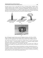
Fig. 10. Context configuration obtained by the proposed method in five different bitplanes of
the image “1230c1G”: (a) when encoding bitplane 14 (seven bits of context); (b) when encoding
bitplane 13 (11 bits of context); (c) when encoding bitplane 12 (13 bits of context); (d) when
encoding bitplane 11 (17 bits of context); (e) when encoding bitplane 10 (20 bits of context).
Context positions falling outside the image at the image borders are considered as having zero
value.
approximately 21 million pixels) required about 220 minutes to compress when the whole
image was used to performed the search. When we used a region of 256
× 256 pixels, it
required approximately 6 minutes to compress the MicroZip test set (about 2 minutes more
than the image-independent approach). These three images have sizes of 1916
×1872, 5496 ×
1956 and 3625 ×1929 pixels. Decoding is faster, because the decoder does not have to search
for the best context: that information is embedded in the bitstream.
6. Experimental results
Table 4 shows the average compression results, in bits per pixel, for the three sets of images
described previously (see Section 3). In this table, we present experimental results of both the
image-independent and the image-dependent approaches. We also include results obtained
with SPIHT (Said and Pearlman, 1996)

4
and EIDAC (Yoo et al., 1998).
Comparing with the results presented in Table 1, we can see that the fast version of the image-
dependent method (indicated as “256
×256” in the table) is 6.3% better than JBIG, 4.7% bet-
ter than JPEG-LS and 8.6% better than lossless JPEG2000. It is important to remember that
JPEG-LS does not provide progressive decoding, a characteristic that is intrinsic to the image-
dependent multi-bitplane finite-context method and also to JPEG2000 and JBIG. From the re-
sults presented in Table 4, it can also be seen that using an area of 256
×256 pixels in the center
of the image for finding the context, instead of the whole image, leads to a small degradation
in the performance (about 0.3%), showing the appropriateness of this approach.
4
SPIHT codec from (version 8.01).
Image set SPIHT EIDAC Image Image-dependent
independent 256
×256 Full
APO_AI 10.812 10.543 10.280 10.225 10.194
ISREC 11.098 10.446 10.199 10.198 10.158
MicroZip 9.198 8.837 8.840 8.667 8.619
Average 10.378 10.005 9.826 9.741 9.708
Table 4. Average compression results, in bits per pixel, using SPIHT, EIDAC, the image-
independent and the image-dependent methods. The “256
× 256” column indicates results
obtained with a context model adjusted using only a square of 256
×256 pixels at the center
of the microarray image, whereas “Full” indicates that the search was performed in the whole
image. The average results presented take into account the different sizes of the images, i.e.,
they correspond to the total number of bits divided by the total number of image pixels.
Table 5 confirms the performance of the image-dependent method relatively to two recent

specialized methods for compressing microarray images: MicroZip (Lonardi and Luo, 2004)
and Zhang’s method (Adjeroh et al., 2006; Zhang et al., 2005). As can be observed, the image-
dependent multi-bitplane finite-context method provides compression gains of 9.1% relatively
to MicroZip and 6.2% in relation to Zhang’s method, on a set of test images that has been used
by all these methods.
Images MicroZip Zhang Image Image-dependent
independent 256
×256 Full
array1 11.490 11.380 11.105 11.120 11.056
array2 9.570 9.260 8.628 8.470 8.423
array3 8.470 8.120 7.962 7.717 7.669
Average 9.532 9.243 8.840 8.667 8.619
Table 5. Compression results, in bits per pixel, using two specialized methods, MicroZip
and Zhang’s method, the image-independent method and the image-dependent method. The
“256
× 256” column indicates results obtained with a context model adjusted using only a
square of 256
×256 pixels at the center of the microarray image, whereas “Full” indicates that
the search was performed in the whole image.
Figure 11 shows, for three different images, the average number of bits per pixel that are
needed for representing each bitplane. As expected, this value generally increases when
going from most significant bitplanes to least significant bitplanes. For the case of images
“Def661Cy3” and “1230c1G”, it can be seen that the average number of bits per pixel re-
quired by the eight least significant bitplanes is close to one, as pointed out by Jörnsten et al.
(2003). However, image “array3” shows a different behavior. Because this image is less
noisy, the compression algorithm is able to exploit redundancies even in lower bitplanes. This
is done without compromising the compression efficiency of noisy images, due to the mech-
anism that monitors and controls the average number of bits per pixel required for encoding
each bitplane.
The maximum number of context bits that we allowed for building the contexts was limited

to 20. Since the coding alphabet is binary, this implies, at most, 2
×2
20
= 2 097 152 counters
that can be stored in approximately 8 MBytes of computer memory. In a 2 GHz Pentium 4
Compressionofmicroarrayimages 445
(a) BP = 14
(b) BP = 13
?
?
?
?
(c) BP = 12
?
(d) BP = 11
(e) BP = 10
Fig. 10. Context configuration obtained by the proposed method in five different bitplanes of
the image “1230c1G”: (a) when encoding bitplane 14 (seven bits of context); (b) when encoding
bitplane 13 (11 bits of context); (c) when encoding bitplane 12 (13 bits of context); (d) when
encoding bitplane 11 (17 bits of context); (e) when encoding bitplane 10 (20 bits of context).
Context positions falling outside the image at the image borders are considered as having zero
value.
approximately 21 million pixels) required about 220 minutes to compress when the whole
image was used to performed the search. When we used a region of 256
× 256 pixels, it
required approximately 6 minutes to compress the MicroZip test set (about 2 minutes more
than the image-independent approach). These three images have sizes of 1916
×1872, 5496 ×
1956 and 3625 ×1929 pixels. Decoding is faster, because the decoder does not have to search
for the best context: that information is embedded in the bitstream.

6. Experimental results
Table 4 shows the average compression results, in bits per pixel, for the three sets of images
described previously (see Section 3). In this table, we present experimental results of both the
image-independent and the image-dependent approaches. We also include results obtained
with SPIHT (Said and Pearlman, 1996)
4
and EIDAC (Yoo et al., 1998).
Comparing with the results presented in Table 1, we can see that the fast version of the image-
dependent method (indicated as “256
×256” in the table) is 6.3% better than JBIG, 4.7% bet-
ter than JPEG-LS and 8.6% better than lossless JPEG2000. It is important to remember that
JPEG-LS does not provide progressive decoding, a characteristic that is intrinsic to the image-
dependent multi-bitplane finite-context method and also to JPEG2000 and JBIG. From the re-
sults presented in Table 4, it can also be seen that using an area of 256
×256 pixels in the center
of the image for finding the context, instead of the whole image, leads to a small degradation
in the performance (about 0.3%), showing the appropriateness of this approach.
4
SPIHT codec from (version 8.01).
Image set SPIHT EIDAC Image Image-dependent
independent 256×256 Full
APO_AI 10.812 10.543 10.280 10.225 10.194
ISREC
11.098 10.446 10.199 10.198 10.158
MicroZip
9.198 8.837 8.840 8.667 8.619
Average 10.378 10.005 9.826 9.741 9.708
Table 4. Average compression results, in bits per pixel, using SPIHT, EIDAC, the image-
independent and the image-dependent methods. The “256
× 256” column indicates results

obtained with a context model adjusted using only a square of 256
×256 pixels at the center
of the microarray image, whereas “Full” indicates that the search was performed in the whole
image. The average results presented take into account the different sizes of the images, i.e.,
they correspond to the total number of bits divided by the total number of image pixels.
Table 5 confirms the performance of the image-dependent method relatively to two recent
specialized methods for compressing microarray images: MicroZip (Lonardi and Luo, 2004)
and Zhang’s method (Adjeroh et al., 2006; Zhang et al., 2005). As can be observed, the image-
dependent multi-bitplane finite-context method provides compression gains of 9.1% relatively
to MicroZip and 6.2% in relation to Zhang’s method, on a set of test images that has been used
by all these methods.
Images MicroZip Zhang Image Image-dependent
independent 256×256 Full
array1 11.490 11.380 11.105 11.120 11.056
array2
9.570 9.260 8.628 8.470 8.423
array3
8.470 8.120 7.962 7.717 7.669
Average 9.532 9.243 8.840 8.667 8.619
Table 5. Compression results, in bits per pixel, using two specialized methods, MicroZip
and Zhang’s method, the image-independent method and the image-dependent method. The
“256
× 256” column indicates results obtained with a context model adjusted using only a
square of 256
×256 pixels at the center of the microarray image, whereas “Full” indicates that
the search was performed in the whole image.
Figure 11 shows, for three different images, the average number of bits per pixel that are
needed for representing each bitplane. As expected, this value generally increases when
going from most significant bitplanes to least significant bitplanes. For the case of images
“Def661Cy3” and “1230c1G”, it can be seen that the average number of bits per pixel re-

quired by the eight least significant bitplanes is close to one, as pointed out by Jörnsten et al.
(2003). However, image “array3” shows a different behavior. Because this image is less
noisy, the compression algorithm is able to exploit redundancies even in lower bitplanes. This
is done without compromising the compression efficiency of noisy images, due to the mech-
anism that monitors and controls the average number of bits per pixel required for encoding
each bitplane.
The maximum number of context bits that we allowed for building the contexts was limited
to 20. Since the coding alphabet is binary, this implies, at most, 2
×2
20
= 2 097 152 counters
that can be stored in approximately 8 MBytes of computer memory. In a 2 GHz Pentium 4
SignalProcessing446
0
0.1
0.2
0.3
0.4
0.5
0.6
0.7
0.8
0.9
1
0 2 4 6 8 10 12 14 16
bpp
Bitplane
Def661Cy3
1230c1G
array3

Fig. 11. Average number of bits per pixel required for encoding each bitplane of three different
microarray images (one from each test set).
computer with 512 MBytes of memory, the image-dependent algorithm required about six
minutes to compress the MicroZip test set (note that this compression time is only indicative,
because the code has not been optimized for speed). Decoding is faster, because the decoder
does not have to search for the best context. Just for comparison, the codecs of the compression
standards took approximately one minute to encode the same set of images.
7. Conclusions
The use of microarray expression data in state-of-the-art biology has been well established.
The widespread adoption of this technology, coupled with the significant volume of data gen-
erated per experiment, in the form of images, has led to significant challenges in storage and
query-retrieval. In this work, we have studied the problem of coding this type of images.
We presented a set of comprehensive results regarding the lossless compression of microar-
ray images by state-of-the-art image coding standards, namely, lossless JPEG2000, JBIG and
JPEG-LS. From the experimental results obtained, we conclude that JPEG-LS gives the best
lossless compression performance. However, it lacks lossy-to-lossless capability, which may
be a decisive functionality if remote transmission over possibly slow links is a requirement.
Complying to this requirement we find JBIG and lossless JPEG2000, lossless JPEG2000 being
the best considering rate-distortion in the sense of the L
2
-norm and JBIG the most efficient
when considering the L
∞
-norm. Moreover, JBIG is consistently better than lossless JPEG2000
regarding lossless compression ratios.
Motivated by these findings, we have developed efficient methods for lossless compression
of microarray images, allowing progressive, lossy-to-lossless decoding. These methods are
based on bitplane compression using image-independent or image-dependent finite-context
models and arithmetic coding. They do not require griding and/or segmentation as most
of the specialized methods that have been proposed do. This may be an advantage if only

compression is sought, since it reduces the complexity of the method. Moreover, since they
do not require griding, they are robust, for example, against layout changes in spot placement.
The results obtained by the multi-bitplane context-based methods have been compared with
the three image coding standards and with two recent specialized methods: MicroZip and
Zhang’s method. The results obtained show that these new methods have better compression
performance in all image test sets used.
8. References
Adjeroh, D., Y. Zhang, and R. Parthe (2006, February). On denoising and compression of DNA
microarray images. Pattern Recognition 39, 2478–2493.
Bell, T. C., J. G. Cleary, and I. H. Witten (1990). Text compression. Prentice Hall.
Faramarzpour, N. and S. Shirani (2004, March). Lossless and lossy compression of DNA mi-
croarray images. In Proc. of the Data Compression Conf., DCC-2004, Snowbird, Utah,
pp. 538.
Faramarzpour, N., S. Shirani, and J. Bondy (2003, November). Lossless DNA microarray im-
age compression. In Proc. of the 37th Asilomar Conf. on Signals, Systems, and Computers,
2003, Volume 2, pp. 1501–1504.
Hampel, H., R. B. Arps, C. Chamzas, D. Dellert, D. L. Duttweiler, T. Endoh, W. Equitz, F. Ono,
R. Pasco, I. Sebestyen, C. J. Starkey, S. J. Urban, Y. Yamazaki, and T. Yoshida (1992,
April). Technical features of the JBIG standard for progressive bi-level image com-
pression. Signal Processing: Image Communication 4(2), 103–111.
Hegde, P., R. Qi, K. Abernathy, C. Gay, S. Dharap, R. Gaspard, J. Earle-Hughes, E. Snesrud,
N. Lee, and J. Q. (2000, September). A concise guide to cDNA microarray analysis.
Biotechniques 29(3), 548–562.
Hua, J., Z. Liu, Z. Xiong, Q. Wu, and K. Castleman (2003, September). Microarray BASICA:
background adjustment, segmentation, image compression and analysis of microar-
ray images. In Proc. of the IEEE Int. Conf. on Image Processing, ICIP-2003, Volume 1,
Barcelona, Spain, pp. 585–588.
Hua, J., Z. Xiong, Q. Wu, and K. Castleman (2002, October). Fast segmentation and lossy-to-
lossless compression of DNA microarray images. In Proc. of the Workshop on Genomic
Signal Processing and Statistics, GENSIPS, Raleigh, NC.

ISO/IEC (1993, March). Information technology - Coded representation of picture and audio infor-
mation - progressive bi-level image compression. International Standard ISO/IEC 11544
and ITU-T Recommendation T.82.
ISO/IEC (1999). Information technology - Lossless and near-lossless compression of continuous-tone
still images. ISO/IEC 14495–1 and ITU Recommendation T.87.
ISO/IEC (2000a). Information technology - JPEG 2000 image coding system. ISO/IEC International
Standard 15444–1, ITU-T Recommendation T.800.
ISO/IEC (2000b). JBIG2 bi-level image compression standard. International Standard ISO/IEC
14492 and ITU-T Recommendation T.88.
Jörnsten, R., W. Wang, B. Yu, and K. Ramchandran (2003). Microarray image compression:
SLOCO and the effect of information loss. Signal Processing 83, 859–869.
Jörnsten, R. and B. Yu (2000, March). Comprestimation: microarray images in abundance. In
Proc. of the Conf. on Information Sciences, Princeton, NJ.
Jörnsten, R. and B. Yu (2002, July). Compression of cDNA microarray images. In Proc. of the
IEEE Int. Symposium on Biomedical Imaging, ISBI-2002, Washington, DC, pp. 38–41.
Jörnsten, R., B. Yu, W. Wang, and K. Ramchandran (2002a, September). Compression of cDNA
and inkjet microarray images. In Proc. of the IEEE Int. Conf. on Image Processing, ICIP-
2002, Volume 3, Rochester, NY, pp. 961–964.
Compressionofmicroarrayimages 447
0
0.1
0.2
0.3
0.4
0.5
0.6
0.7
0.8
0.9
1

0 2 4 6 8 10 12 14 16
bpp
Bitplane
Def661Cy3
1230c1G
array3
Fig. 11. Average number of bits per pixel required for encoding each bitplane of three different
microarray images (one from each test set).
computer with 512 MBytes of memory, the image-dependent algorithm required about six
minutes to compress the MicroZip test set (note that this compression time is only indicative,
because the code has not been optimized for speed). Decoding is faster, because the decoder
does not have to search for the best context. Just for comparison, the codecs of the compression
standards took approximately one minute to encode the same set of images.
7. Conclusions
The use of microarray expression data in state-of-the-art biology has been well established.
The widespread adoption of this technology, coupled with the significant volume of data gen-
erated per experiment, in the form of images, has led to significant challenges in storage and
query-retrieval. In this work, we have studied the problem of coding this type of images.
We presented a set of comprehensive results regarding the lossless compression of microar-
ray images by state-of-the-art image coding standards, namely, lossless JPEG2000, JBIG and
JPEG-LS. From the experimental results obtained, we conclude that JPEG-LS gives the best
lossless compression performance. However, it lacks lossy-to-lossless capability, which may
be a decisive functionality if remote transmission over possibly slow links is a requirement.
Complying to this requirement we find JBIG and lossless JPEG2000, lossless JPEG2000 being
the best considering rate-distortion in the sense of the L
2
-norm and JBIG the most efficient
when considering the L
∞
-norm. Moreover, JBIG is consistently better than lossless JPEG2000

regarding lossless compression ratios.
Motivated by these findings, we have developed efficient methods for lossless compression
of microarray images, allowing progressive, lossy-to-lossless decoding. These methods are
based on bitplane compression using image-independent or image-dependent finite-context
models and arithmetic coding. They do not require griding and/or segmentation as most
of the specialized methods that have been proposed do. This may be an advantage if only
compression is sought, since it reduces the complexity of the method. Moreover, since they
do not require griding, they are robust, for example, against layout changes in spot placement.
The results obtained by the multi-bitplane context-based methods have been compared with
the three image coding standards and with two recent specialized methods: MicroZip and
Zhang’s method. The results obtained show that these new methods have better compression
performance in all image test sets used.
8. References
Adjeroh, D., Y. Zhang, and R. Parthe (2006, February). On denoising and compression of DNA
microarray images. Pattern Recognition 39, 2478–2493.
Bell, T. C., J. G. Cleary, and I. H. Witten (1990). Text compression. Prentice Hall.
Faramarzpour, N. and S. Shirani (2004, March). Lossless and lossy compression of DNA mi-
croarray images. In Proc. of the Data Compression Conf., DCC-2004, Snowbird, Utah,
pp. 538.
Faramarzpour, N., S. Shirani, and J. Bondy (2003, November). Lossless DNA microarray im-
age compression. In Proc. of the 37th Asilomar Conf. on Signals, Systems, and Computers,
2003, Volume 2, pp. 1501–1504.
Hampel, H., R. B. Arps, C. Chamzas, D. Dellert, D. L. Duttweiler, T. Endoh, W. Equitz, F. Ono,
R. Pasco, I. Sebestyen, C. J. Starkey, S. J. Urban, Y. Yamazaki, and T. Yoshida (1992,
April). Technical features of the JBIG standard for progressive bi-level image com-
pression. Signal Processing: Image Communication 4(2), 103–111.
Hegde, P., R. Qi, K. Abernathy, C. Gay, S. Dharap, R. Gaspard, J. Earle-Hughes, E. Snesrud,
N. Lee, and J. Q. (2000, September). A concise guide to cDNA microarray analysis.
Biotechniques 29(3), 548–562.
Hua, J., Z. Liu, Z. Xiong, Q. Wu, and K. Castleman (2003, September). Microarray BASICA:

background adjustment, segmentation, image compression and analysis of microar-
ray images. In Proc. of the IEEE Int. Conf. on Image Processing, ICIP-2003, Volume 1,
Barcelona, Spain, pp. 585–588.
Hua, J., Z. Xiong, Q. Wu, and K. Castleman (2002, October). Fast segmentation and lossy-to-
lossless compression of DNA microarray images. In Proc. of the Workshop on Genomic
Signal Processing and Statistics, GENSIPS, Raleigh, NC.
ISO/IEC (1993, March). Information technology - Coded representation of picture and audio infor-
mation - progressive bi-level image compression. International Standard ISO/IEC 11544
and ITU-T Recommendation T.82.
ISO/IEC (1999). Information technology - Lossless and near-lossless compression of continuous-tone
still images. ISO/IEC 14495–1 and ITU Recommendation T.87.
ISO/IEC (2000a). Information technology - JPEG 2000 image coding system. ISO/IEC International
Standard 15444–1, ITU-T Recommendation T.800.
ISO/IEC (2000b). JBIG2 bi-level image compression standard. International Standard ISO/IEC
14492 and ITU-T Recommendation T.88.
Jörnsten, R., W. Wang, B. Yu, and K. Ramchandran (2003). Microarray image compression:
SLOCO and the effect of information loss. Signal Processing 83, 859–869.
Jörnsten, R. and B. Yu (2000, March). Comprestimation: microarray images in abundance. In
Proc. of the Conf. on Information Sciences, Princeton, NJ.
Jörnsten, R. and B. Yu (2002, July). Compression of cDNA microarray images. In Proc. of the
IEEE Int. Symposium on Biomedical Imaging, ISBI-2002, Washington, DC, pp. 38–41.
Jörnsten, R., B. Yu, W. Wang, and K. Ramchandran (2002a, September). Compression of cDNA
and inkjet microarray images. In Proc. of the IEEE Int. Conf. on Image Processing, ICIP-
2002, Volume 3, Rochester, NY, pp. 961–964.
SignalProcessing448
Jörnsten, R., B. Yu, W. Wang, and K. Ramchandran (2002b, October). Microarray image com-
pression and the effect of compression loss. In Proc. of the Workshop on Genomic Signal
Processing and Statistics, GENSIPS, Raleigh, NC.
Kothapalli, R., S. J. Yoder, S. Mane, and T. P. L. Jr (2002). Microarray results: how accurate are
they? BMC Bioinformatics 3.

Leung, Y. F. and D. Cavalieri (2003, November). Fundamentals of cDNA microarray data
analysis. Trends on Genetics 19(11), 649–659.
Lonardi, S. and Y. Luo (2004, August). Gridding and compression of microarray images. In
Proc. of the IEEE Computational Systems Bioinformatics Conference, CSB-2004, Stanford,
CA.
Moore, S. K. (2001, March). Making chips to probe genes. IEEE Spectrum 38(3), 54–60.
Netravali, A. N. and B. G. Haskell (1995). Digital pictures: representation, compression and stan-
dards (2nd ed.). New York: Plenum.
Neves, A. J. R. and A. J. Pinho (2006, October). Lossless compression of microarray images. In
Proc. of the IEEE Int. Conf. on Image Processing, ICIP-2006, Atlanta, GA, pp. 2505–2508.
Neves, A. J. R. and A. J. Pinho (2009, February). Lossless compression of microarray images
using image-dependent finite-context models. IEEE Trans. on Medical Imaging 28(2),
194–201.
Pinho, A. J. and A. J. R. Neves (2006, October). Lossy-to-lossless compression of images based
on binary tree decomposition. In Proc. of the IEEE Int. Conf. on Image Processing, ICIP-
2006, Atlanta, GA, pp. 2257–2260.
Rissanen, J. (1983, September). A universal data compression system. IEEE Trans. on Informa-
tion Theory 29(5), 656–664.
Rissanen, J. and G. G. Langdon, Jr. (1981, January). Universal modeling and coding. IEEE
Trans. on Information Theory 27(1), 12–23.
Said, A. and W. A. Pearlman (1996, June). A new, fast, and efficient image codec based on
set partitioning in hierarchical trees. IEEE Trans. on Circuits and Systems for Video
Technology 6(3), 243–250.
Salomon, D. (2000). Data compression - The complete reference (2nd ed.). Springer.
Sasik, R., C. H. Woelk, and J. Corbeil (2004, August). Microarray truths and consequences.
Journal of Molecular Endocrinology 33(1), 1–9.
Sayood, K. (2000). Introduction to data compression (2nd ed.). Morgan Kaufmann.
Skodras, A., C. Christopoulos, and T. Ebrahimi (2001, September). The JPEG 2000 still image
compression standard. IEEE Signal Processing Magazine 18(5), 36–58.
Taubman, D. S. and M. W. Marcellin (2002). JPEG 2000: image compression fundamentals, stan-

dards and practice. Kluwer Academic Publishers.
Weinberger, M. J., G. Seroussi, and G. Sapiro (2000, August). The LOCO-I lossless image
compression algorithm: principles and standardization into JPEG-LS. IEEE Trans. on
Image Processing 9(8), 1309–1324.
Yoo, Y., Y. G. Kwon, and A. Ortega (1998, November). Embedded image-domain adaptive
compression of simple images. In Proc. of the 32nd Asilomar Conf. on Signals, Systems,
and Computers, Volume 2, Pacific Grove, CA, pp. 1256–1260.
Zhang, Y., R. Parthe, and D. Adjeroh (2005, August). Lossless compression of DNA microarray
images. In Proc. of the IEEE Computational Systems Bioinformatics Conference, CSB-2005,
Stanford, CA.
RoundoffNoiseMinimizationforState-EstimateFeedback
DigitalControllersUsingJointOptimizationofErrorFeedbackandRealization 449
Roundoff Noise Minimization for State-Estimate Feedback Digital
ControllersUsingJointOptimizationofErrorFeedbackandRealization
TakaoHinamoto,KeijiroKawai,MasayoshiNakamotoandWu-ShengLu
0
Roundoff Noise Minimization for State-Estimate
Feedback Digital Controllers Using Joint
Optimization of Error Feedback and Realization
Takao Hinamoto, Keijiro Kawai, Masayoshi Nakamoto and Wu-Sheng Lu
Name-of-the-University-Company
Country
1. INTRODUCTION
Due to the finite precision nature of computer arithmetic, the output roundoff noise of a fixed-
point IIR digital filter usually arises. This noise is critically dependent on the internal structure
of an IIR digital filter [1],[2]. Error feedback (EF) is known as an effective technique for reduc-
ing the output roundoff noise in an IIR digital filter [3]-[5]. Williamson [6] has reduced the
output roundoff noise more effectively by choosing the filter structure and applying EF to the
filter. Lu and Hinamoto [7] have developed a jointly optimized technique of EF and realiza-
tion to minimize the effects of roundoff noise at the filter output subject to l

2
-norm dynamic-
range scaling constraints. Li and Gevers [8] have analyzed the output roundoff noise of the
closed-loop system with a state-estimate feedback controller, and presented an algorithm for
realizing the state-estimate feedback controller with minimum output roundoff noise under
l
2
-norm dynamic-range scaling constraints. Hinamoto and Yamamoto [9] have proposed a
method for applying EF to a given closed-loop system with a state-estimate feedback con-
troller.
This paper investigates the problem of jointly optimizing EF and realization for the closed-
loop system with a state-estimate feedback controller so as to minimize the output roundoff
noise subject to l
2
-norm dynamic-range scaling constraints. To this end, the problem at hand is
converted into an unconstrained optimization problem by using linear-algebraic techniques,
and then an iterative technique which relies on a quasi-Newton algorithm [10] is developed.
With a closed-form formula for gradient evaluation and an efficient quasi-Newton solver, the
unconstrained optimization problem can be solved efficiently. Our computer simulation re-
sults demonstrate the validity and effectiveness of the proposed technique.
Throughout the paper, I
n
stands for the identity matrix of dimension n × n, the transpose
(conjugate transpose) of a matrix A is indicated by A
T
(A
∗
), and the trace and ith diagonal
element of a square matrix A are denoted by tr
[A] and (A)

ii
, respectively.
2. ROUNDOFF NOISE ANALYSIS
Consider a stable, controllable and observable linear discrete-time system described by
x
(k + 1) = A
o
x(k) + b
o
u(k)
y(k) = c
o
x(k)
(1)
23
SignalProcessing450
where x(k) is an n ×1 state-variable vector, u(k) is a scalar input, y(k) is a scalar output, and
A
o
, b
o
and c
o
are n × n, n × 1 and 1 × n real constant matrices, respectively. The transfer
function of the linear system in (1) is given by
H
o
(z) = c
o
(zI

n
− A
o
)
−1
b
o
. (2)
If a regulator is designed by using the full-order state observer, we obtain a state-estimate
feedback controller as
˜x
(k + 1) = F
o
˜x(k) + b
o
u(k) + g
o
y(k)
=
R
o
˜x(k) + b
o
r(k) + g
o
y(k)
u(k) = − k
o
˜x(k) + r(k)
(3)

where ˜x
(k) is an n ×1 state-variable vector in the full-order state observer, g
o
is an n ×1 gain
vector chosen so that all the eigenvalues of F
o
= A
o
− g
o
c
o
are inside the unit circle in the
complex plane, k
o
is a 1 ×n state-feedback gain vector chosen so that each of the eigenvalues
of A
o
− b
o
k
o
is at a desirable location within the unit circle, r(k) is a scalar reference signal,
and R
o
= F
o
−b
o
k

o
. The closed-loop control system consisting of the linear system in (1) and
the state-estimate feedback controller in (3) is illustrated in Fig. 1.
~
u(k)r(k) y(k)
HO(z)
x(k)
z
-1
I
O
FO
kO
bO
g
Fig. 1. The closed-loop control system with a state-estimate feedback controller.
When performing quantization before matrix-vector multiplication, we can express the finite-
word-length (FWL) implementation of (3) with error feedback as
ˆx
(k + 1) = R Q[ˆx(k)] + br(k) + gy(k) + De(k)
u(k) = − k Q[ˆx(k)] + r( k)
(4)
where
e
(k) = ˆx(k) − Q[ˆx(k)]
is an n × 1 roundoff error vector and D is an n × n error feedback matrix. All coefficient
matrices R, b, g and k are assumed to have an exact fractional B
c
bit representation. The FWL
state-variable vector ˆx(k) and signal u(k) all have a B bit fractional representation, while the

reference input r
(k) is a (B − B
c
) bit fraction. The vector quantizer Q[·] in (4) rounds the B
bit fraction ˆx
(k) to (B − B
c
) bits after completing the multiplications and additions, where the
sign bit is not counted. It is assumed that the roundoff error vector e
(k) can be modeled as a
zero-mean noise process with covariance σ
2
I
n
where
σ
2
=
1
12
2
−2(B−B
c
)
.
It is noted that if the ith element of the roundoff error vector e
(k) is indicated by e
i
(k) for i =
1, 2, ··· , n then the variable e

i
(k) can be approximated by a white noise sequence uniformly
distributed with the following probability density function:
p
(e
i
(k)) =

2
B−B
c
for −
1
2
2
−(B−B
c
)
≤ e
i
(k) ≤
1
2
2
−(B−B
c
)
0 otherwise
u(k)r(k) y(k)
HO(z)

z
-1
I
R
k
b
g
Q
D
e(k)
^
x(k)
^
[x(k)]
Q
Fig. 2. A state-estimate feedback controller with error feedback.
The closed-loop system consisting of the linear system in (1) and the state-estimate feedback
controller with error feedback in (4) is shown in Fig. 2, and is described by

x
(k + 1)
ˆx(k + 1)

= A

x
(k)
ˆx(k)

+ br(k) + Be(k)

y(k) = c

x
(k)
ˆx(k)

(5)
RoundoffNoiseMinimizationforState-EstimateFeedback
DigitalControllersUsingJointOptimizationofErrorFeedbackandRealization 451
where x(k) is an n ×1 state-variable vector, u(k) is a scalar input, y(k) is a scalar output, and
A
o
, b
o
and c
o
are n × n, n × 1 and 1 × n real constant matrices, respectively. The transfer
function of the linear system in (1) is given by
H
o
(z) = c
o
(zI
n
− A
o
)
−1
b
o

. (2)
If a regulator is designed by using the full-order state observer, we obtain a state-estimate
feedback controller as
˜x
(k + 1) = F
o
˜x(k) + b
o
u(k) + g
o
y(k)
=
R
o
˜x(k) + b
o
r(k) + g
o
y(k)
u(k) = − k
o
˜x(k) + r(k)
(3)
where ˜x
(k) is an n ×1 state-variable vector in the full-order state observer, g
o
is an n ×1 gain
vector chosen so that all the eigenvalues of F
o
= A

o
− g
o
c
o
are inside the unit circle in the
complex plane, k
o
is a 1 ×n state-feedback gain vector chosen so that each of the eigenvalues
of A
o
− b
o
k
o
is at a desirable location within the unit circle, r(k) is a scalar reference signal,
and R
o
= F
o
−b
o
k
o
. The closed-loop control system consisting of the linear system in (1) and
the state-estimate feedback controller in (3) is illustrated in Fig. 1.
~
u(k)r(k) y(k)
HO(z)
x(k)

z
-1
I
O
FO
kO
bO
g
Fig. 1. The closed-loop control system with a state-estimate feedback controller.
When performing quantization before matrix-vector multiplication, we can express the finite-
word-length (FWL) implementation of (3) with error feedback as
ˆx
(k + 1) = R Q[ˆx(k)] + br(k) + gy(k) + De(k)
u(k) = − k Q[ˆx(k)] + r( k)
(4)
where
e
(k) = ˆx(k) − Q[ˆx(k)]
is an n × 1 roundoff error vector and D is an n × n error feedback matrix. All coefficient
matrices R, b, g and k are assumed to have an exact fractional B
c
bit representation. The FWL
state-variable vector ˆx(k) and signal u(k) all have a B bit fractional representation, while the
reference input r
(k) is a (B − B
c
) bit fraction. The vector quantizer Q[·] in (4) rounds the B
bit fraction ˆx
(k) to (B − B
c

) bits after completing the multiplications and additions, where the
sign bit is not counted. It is assumed that the roundoff error vector e
(k) can be modeled as a
zero-mean noise process with covariance σ
2
I
n
where
σ
2
=
1
12
2
−2(B−B
c
)
.
It is noted that if the ith element of the roundoff error vector e
(k) is indicated by e
i
(k) for i =
1, 2, ··· , n then the variable e
i
(k) can be approximated by a white noise sequence uniformly
distributed with the following probability density function:
p
(e
i
(k)) =


2
B−B
c
for −
1
2
2
−(B−B
c
)
≤ e
i
(k) ≤
1
2
2
−(B−B
c
)
0 otherwise
u(k)r(k) y(k)
HO(z)
z
-1
I
R
k
b
g

Q
D
e(k)
^
x(k)
^
[x(k)]
Q
Fig. 2. A state-estimate feedback controller with error feedback.
The closed-loop system consisting of the linear system in (1) and the state-estimate feedback
controller with error feedback in (4) is shown in Fig. 2, and is described by

x
(k + 1)
ˆx(k + 1)

= A

x
(k)
ˆx(k)

+ br(k) + Be(k)
y(k) = c

x
(k)
ˆx(k)

(5)

SignalProcessing452
where
A =

A
o
−b
o
k
gc
o
R

,
b =

b
o
b

B =

b
o
k
D
− R

,
c =

[
c
o
0
]
.
From (5), the transfer function from the roundoff error vector e
(k) to the output y(k) is given
by
G
D
(z) = c (zI
2n
− A)
−1
B. (6)
The output noise gain J
(D) = σ
2
out
/σ
2
is then computed as
J
(D) = tr[W
D
] (7)
with
W
D

=
1
2πj

|z|=1
G
∗
D
(z)G
D
(z)
dz
z
(8)
where σ
2
out
stands for the noise variance at the output. For tractability, we evaluate J(D) in (7)
by replacing R, b, g and k by R
o
, b
o
, g
o
and k
o
, respectively. Defining
S
=


I
n
0
I
n
−I
n

, (9)
the transfer function in (6) can be expressed as
G
D
(z) =
cS(zI
2n
−S
−1
AS)
−1
S
−1
B
=
c(zI
2n
−Φ)
−1

b
o

k
o
F
o
− D

= c
o
(zI
n
− A
o
+ b
o
k
o
)
−1
b
o
k
o
(zI
n
− F
o
)
−1
·(zI
n

− D)
=
c(zI
2n
−Φ)
−1
U(zI
n
− D)
(10)
where
Φ
=

A
o
−b
o
k
o
b
o
k
o
0 F
o

U
=


0
I
n

.
It is noted that the stability of the closed-loop control system is determined by the eigenvalues
of matrix
A in (5), or equivalently, those of matrix Φ in (10). This means that neither of the
roundoff error vector e
(k) and the error-feedback matrix D affects the stability.
Substituting (10) into matrix W
D
in (8) gives
W
D
= (b
0
k
0
)
T
W
1
b
0
k
0
+ (b
0
k

0
)
T
W
2
(F
0
− D)
+(
F
0
− D)
T
W
3
b
0
k
0
+(F
0
− D)
T
W
4
(F
0
− D)
(11)
where

W
= Φ
T
WΦ +
c
T
c
W
=

W
1
W
2
W
3
W
4

.
Since W is positive semidefinite, it can be shown that there exists an n
×n matrix P such that
W
3
= W
4
P. In addition, (11) can be written by virtue of W
2
= W
T

3
as
W
D
= (F
0
+ Pb
0
k
0
− D)
T
W
4
(F
0
+ Pb
0
k
0
− D)
+(
b
0
k
0
)
T
(W
1

−P
T
W
4
P)b
0
k
0
.
(12)
Alternatively, applying z-transform to the first equation in (5) under the assumption that
e
(k) = 0, we obtain

X
(z)
ˆ
X
(z)

= (zI − A)
−1
bR(z) (13)
where X
(z),
ˆ
X(z) and R(z) represent the z-transforms of x(k), ˆx(k) and r(k), respectively.
Replacing R, b, k and g by R
o
, b

o
, k
o
and g
o
, respectively, and then using
S
−1

X
(z)
ˆ
X
(z)

= (zI
2n
−S
−1
AS)
−1
S
−1
b
yields
ˆ
X
(z) = X(z) = F(z)R(z) (14)
where
F

(z) = [zI
n
−(A
o
−b
o
k
o
)]
−1
b
o
.
The controllability Gramian K defined by
K
=
1
2πj

|z|=1
F(z)F
∗
(z)
dz
z
(15)
can be obtained by solving the following Lyapunov equation:
K
= (A
o

−b
o
k
o
)K(A
o
−b
o
k
o
)
T
+ b
o
b
T
o
. (16)
3. ROUNDOFF NOISE MINIMIZATION
Consider the system in (4) with D = 0 and denote it by (R, b, g, k)
n
. By applying a coordinate
transformation ˜x

(k) = T
−1
ˆx(k) to the above system (R , b, g, k)
n
, we obtain a new realization
characterized by

(
˜
R,
˜
b, ˜g,
˜
k
)
n
where
˜
R
= T
−1
RT,
˜
b = T
−1
b
˜g
= T
−1
g,
˜
k = kT.
(17)
For the system described by (17), the counterparts of W
i
for i = 1, 2, 3,4 are given by
˜

W
i
= T
T
W
i
T (18)
RoundoffNoiseMinimizationforState-EstimateFeedback
DigitalControllersUsingJointOptimizationofErrorFeedbackandRealization 453
where
A
=

A
o
−b
o
k
gc
o
R

, b
=

b
o
b

B

=

b
o
k
D
− R

, c
=
[
c
o
0
]
.
From (5), the transfer function from the roundoff error vector e
(k) to the output y(k) is given
by
G
D
(z) = c (zI
2n
− A)
−1
B. (6)
The output noise gain J
(D) = σ
2
out

/σ
2
is then computed as
J
(D) = tr[W
D
] (7)
with
W
D
=
1
2πj

|z|=1
G
∗
D
(z)G
D
(z)
dz
z
(8)
where σ
2
out
stands for the noise variance at the output. For tractability, we evaluate J(D) in (7)
by replacing R, b, g and k by R
o

, b
o
, g
o
and k
o
, respectively. Defining
S
=

I
n
0
I
n
−I
n

, (9)
the transfer function in (6) can be expressed as
G
D
(z) =
cS(zI
2n
−S
−1
AS)
−1
S

−1
B
=
c(zI
2n
−Φ)
−1

b
o
k
o
F
o
− D

= c
o
(zI
n
− A
o
+ b
o
k
o
)
−1
b
o

k
o
(zI
n
− F
o
)
−1
·(zI
n
− D)
=
c(zI
2n
−Φ)
−1
U(zI
n
− D)
(10)
where
Φ
=

A
o
−b
o
k
o

b
o
k
o
0 F
o

U
=

0
I
n

.
It is noted that the stability of the closed-loop control system is determined by the eigenvalues
of matrix A in (5), or equivalently, those of matrix Φ in (10). This means that neither of the
roundoff error vector e
(k) and the error-feedback matrix D affects the stability.
Substituting (10) into matrix W
D
in (8) gives
W
D
= (b
0
k
0
)
T

W
1
b
0
k
0
+ (b
0
k
0
)
T
W
2
(F
0
− D)
+(
F
0
− D)
T
W
3
b
0
k
0
+(F
0

− D)
T
W
4
(F
0
− D)
(11)
where
W
= Φ
T
WΦ +
c
T
c
W
=

W
1
W
2
W
3
W
4

.
Since W is positive semidefinite, it can be shown that there exists an n

×n matrix P such that
W
3
= W
4
P. In addition, (11) can be written by virtue of W
2
= W
T
3
as
W
D
= (F
0
+ Pb
0
k
0
− D)
T
W
4
(F
0
+ Pb
0
k
0
− D)

+(
b
0
k
0
)
T
(W
1
−P
T
W
4
P)b
0
k
0
.
(12)
Alternatively, applying z-transform to the first equation in (5) under the assumption that
e
(k) = 0, we obtain

X
(z)
ˆ
X
(z)

= (zI − A)

−1
bR(z) (13)
where X
(z),
ˆ
X(z) and R(z) represent the z-transforms of x(k), ˆx(k) and r(k), respectively.
Replacing R, b, k and g by R
o
, b
o
, k
o
and g
o
, respectively, and then using
S
−1

X
(z)
ˆ
X
(z)

= (zI
2n
−S
−1
AS)
−1

S
−1
b
yields
ˆ
X
(z) = X(z) = F(z)R(z) (14)
where
F
(z) = [zI
n
−(A
o
−b
o
k
o
)]
−1
b
o
.
The controllability Gramian K defined by
K
=
1
2πj

|z|=1
F(z)F

∗
(z)
dz
z
(15)
can be obtained by solving the following Lyapunov equation:
K
= (A
o
−b
o
k
o
)K(A
o
−b
o
k
o
)
T
+ b
o
b
T
o
. (16)
3. ROUNDOFF NOISE MINIMIZATION
Consider the system in (4) with D = 0 and denote it by (R, b, g, k)
n

. By applying a coordinate
transformation ˜x

(k) = T
−1
ˆx(k) to the above system (R , b, g, k)
n
, we obtain a new realization
characterized by
(
˜
R,
˜
b, ˜g,
˜
k
)
n
where
˜
R
= T
−1
RT,
˜
b = T
−1
b
˜g
= T

−1
g,
˜
k = kT.
(17)
For the system described by (17), the counterparts of W
i
for i = 1, 2, 3,4 are given by
˜
W
i
= T
T
W
i
T (18)
SignalProcessing454
and the corresponding output noise gain is given by
J
(D, T) = tr[
˜
W
D
] (19)
where
˜
W
D
can be obtained referring to (11) as
˜

W
D
=

T
−1
(F
0
+ Pb
0
k
0
)T − D

T
·T
T
W
4
T

T
−1
(F
0
+ Pb
0
k
0
)T − D


+T
T
(b
0
k
0
)
T
(W
1
−P
T
W
4
P)b
0
k
0
T.
In addition, (15) can be written as
˜
K
=
1
2πj

|z|=1
T
−1

F(z)F
∗
(z)T
−T
dz
z
= T
−1
KT
−T
.
(20)
As a result, the output roundoff noise minimization problem amounts to obtaining matrices
D and T which jointly minimize J
(D, T) in (19) subject to the l
2
-norm dynamic-range scaling
constraints specified by
(
˜
K
)
ii
= (T
−1
KT
−T
)
ii
= 1, i = 1, 2, ··· , n. (21)

To deal with (21), we define
ˆ
T
= T
T
K
−
1
2
. (22)
Then the l
2
-norm dynamic-range scaling constraints in (21) can be written as
(
ˆ
T
−T
ˆ
T
−1
)
ii
= 1, i = 1, 2, ··· , n. (23)
These constraints are always satisfied if
ˆ
T
−1
assumes the form
ˆ
T

−1
=

t
1
||
t
1
||
,
t
2
||
t
2
||
, ··· ,
t
n
||
t
n
||

. (24)
Substituting (22) into (19), we obtain
J
(D,
ˆ
T) = tr


ˆ
T(
ˆ
A
−
ˆ
T
T
D
ˆ
T
−T
)
T
ˆ
W
4
·(
ˆ
A
−
ˆ
T
T
D
ˆ
T
−T
)

ˆ
T
T
+
ˆ
T
ˆ
C
ˆ
T
T

(25)
where
ˆ
A
= K
−
1
2
(F
0
+ Pb
0
k
0
)K
1
2
,

ˆ
W
4
= K
1
2
W
4
K
1
2
ˆ
C
= K
1
2
(b
0
k
0
)
T
(W
1
−P
T
W
4
P)b
0

k
0
K
1
2
.
From the foregoing arguments, the problem of obtaining matrices D and T that minimize (19)
subject to the scaling constraints in (21) is now converted into an unconstrained optimization
problem of obtaining D and
ˆ
T that jointly minimize J
(D,
ˆ
T) in (25).
Let x be the column vector that collects the variables in matrix D and matrix [t
1
, t
2
, ··· , t
n
].
Then J
(D,
ˆ
T) is a function of x, denoted by J(x). The proposed algorithm starts with an initial
point x
0
obtained from an initial assignment D =
ˆ
T

= I
n
. In the kth iteration, a quasi-Newton
algorithm updates the most recent point x
k
to point x
k+1
as [10]
x
k+1
= x
k
+ α
k
d
k
(26)
where
d
k
= −S
k
∇J(x
k
)
α
k
= arg

min

α
J(x
k
+ αd
k
)

S
k+1
= S
k
+

1
+
γ
T
k
S
k
γ
k
γ
T
k
δ
k

δ
k

δ
T
k
γ
T
k
δ
k
−
δ
k
γ
T
k
S
k
+S
k
γ
k
δ
T
k
γ
T
k
δ
k
S
0

= I, δ
k
= x
k+1
−x
k
, γ
k
= ∇J(x
k+1
)−∇J(x
k
).
Here,
∇J(x) is the gradient of J(x) with respect to x, and S
k
is a positive-definite approxima-
tion of the inverse Hessian matrix of J
(x
k
). This iteration process continues until
|J(x
k+1
) − J(x
k
)| < ε (27)
is satisfied where ε
> 0 is a prescribed tolerance.
In what follows, we derive closed-form expressions of
∇J(x) for the cases where D assumes

the form of a general, diagonal, or scalar matrix.
1) Case 1: D Is a General Matrix: From (25), the optimal choice of D is given by
D
=
ˆ
T
−T
ˆ
A
ˆ
T
T
, (28)
which leads to
J
(
ˆ
T
−T
ˆ
A
ˆ
T
T
,
ˆ
T) = tr

ˆ
T

ˆ
C
ˆ
T
T

. (29)
In this case, the number of elements in vector x consisting of
ˆ
T is equal to n
2
and the gradient
of J
(x) is found to be
∂J
(x)
∂t
ij
= lim
∆→0
J(
ˆ
T
ij
) − J(
ˆ
T
)
∆
= 2e

T
j
ˆ
T
ˆ
C
ˆ
T
T
ˆ
Tg
ij
, i, j = 1, 2, ··· , n
(30)
where
ˆ
T
ij
is the matrix obtained from
ˆ
T with a perturbed (i, j)th component, which is given
by
ˆ
T
ij
=
ˆ
T
+
∆

ˆ
Tg
ij
e
T
j
ˆ
T
1
−∆e
T
j
ˆ
Tg
ij
and g
ij
is computed using
g
ij
= ∂

t
j
||t
j
||

/∂t
ij

=
1
||t
j
||
3
(t
ij
t
j
−||t
j
||
2
e
i
).
2) Case 2: D Is a Diagonal Matrix: Here, matrix D assumes the form
D
= diag{d
1
, d
2
, ··· , d
n
}. (31)
RoundoffNoiseMinimizationforState-EstimateFeedback
DigitalControllersUsingJointOptimizationofErrorFeedbackandRealization 455
and the corresponding output noise gain is given by
J

(D, T) = tr[
˜
W
D
] (19)
where
˜
W
D
can be obtained referring to (11) as
˜
W
D
=

T
−1
(F
0
+ Pb
0
k
0
)T − D

T
·T
T
W
4

T

T
−1
(F
0
+ Pb
0
k
0
)T − D

+T
T
(b
0
k
0
)
T
(W
1
−P
T
W
4
P)b
0
k
0

T.
In addition, (15) can be written as
˜
K
=
1
2πj

|z|=1
T
−1
F(z)F
∗
(z)T
−T
dz
z
= T
−1
KT
−T
.
(20)
As a result, the output roundoff noise minimization problem amounts to obtaining matrices
D and T which jointly minimize J
(D, T) in (19) subject to the l
2
-norm dynamic-range scaling
constraints specified by
(

˜
K
)
ii
= (T
−1
KT
−T
)
ii
= 1, i = 1, 2, ··· , n. (21)
To deal with (21), we define
ˆ
T
= T
T
K
−
1
2
. (22)
Then the l
2
-norm dynamic-range scaling constraints in (21) can be written as
(
ˆ
T
−T
ˆ
T

−1
)
ii
= 1, i = 1, 2, ··· , n. (23)
These constraints are always satisfied if
ˆ
T
−1
assumes the form
ˆ
T
−1
=

t
1
||
t
1
||
,
t
2
||
t
2
||
, ··· ,
t
n

||
t
n
||

. (24)
Substituting (22) into (19), we obtain
J
(D,
ˆ
T) = tr

ˆ
T(
ˆ
A
−
ˆ
T
T
D
ˆ
T
−T
)
T
ˆ
W
4
·(

ˆ
A
−
ˆ
T
T
D
ˆ
T
−T
)
ˆ
T
T
+
ˆ
T
ˆ
C
ˆ
T
T

(25)
where
ˆ
A
= K
−
1

2
(F
0
+ Pb
0
k
0
)K
1
2
,
ˆ
W
4
= K
1
2
W
4
K
1
2
ˆ
C
= K
1
2
(b
0
k

0
)
T
(W
1
−P
T
W
4
P)b
0
k
0
K
1
2
.
From the foregoing arguments, the problem of obtaining matrices D and T that minimize (19)
subject to the scaling constraints in (21) is now converted into an unconstrained optimization
problem of obtaining D and
ˆ
T that jointly minimize J
(D,
ˆ
T) in (25).
Let x be the column vector that collects the variables in matrix D and matrix [t
1
, t
2
, ··· , t

n
].
Then J
(D,
ˆ
T) is a function of x, denoted by J(x). The proposed algorithm starts with an initial
point x
0
obtained from an initial assignment D =
ˆ
T
= I
n
. In the kth iteration, a quasi-Newton
algorithm updates the most recent point x
k
to point x
k+1
as [10]
x
k+1
= x
k
+ α
k
d
k
(26)
where
d

k
= −S
k
∇J(x
k
)
α
k
= arg

min
α
J(x
k
+ αd
k
)

S
k+1
= S
k
+

1
+
γ
T
k
S

k
γ
k
γ
T
k
δ
k

δ
k
δ
T
k
γ
T
k
δ
k
−
δ
k
γ
T
k
S
k
+S
k
γ

k
δ
T
k
γ
T
k
δ
k
S
0
= I, δ
k
= x
k+1
−x
k
, γ
k
= ∇J(x
k+1
)−∇J(x
k
).
Here,
∇J(x) is the gradient of J(x) with respect to x, and S
k
is a positive-definite approxima-
tion of the inverse Hessian matrix of J
(x

k
). This iteration process continues until
|J(x
k+1
) − J(x
k
)| < ε (27)
is satisfied where ε
> 0 is a prescribed tolerance.
In what follows, we derive closed-form expressions of
∇J(x) for the cases where D assumes
the form of a general, diagonal, or scalar matrix.
1) Case 1: D Is a General Matrix: From (25), the optimal choice of D is given by
D
=
ˆ
T
−T
ˆ
A
ˆ
T
T
, (28)
which leads to
J
(
ˆ
T
−T

ˆ
A
ˆ
T
T
,
ˆ
T) = tr

ˆ
T
ˆ
C
ˆ
T
T

. (29)
In this case, the number of elements in vector x consisting of
ˆ
T is equal to n
2
and the gradient
of J
(x) is found to be
∂J
(x)
∂t
ij
= lim

∆→0
J(
ˆ
T
ij
) − J(
ˆ
T
)
∆
= 2e
T
j
ˆ
T
ˆ
C
ˆ
T
T
ˆ
Tg
ij
, i, j = 1, 2, ··· , n
(30)
where
ˆ
T
ij
is the matrix obtained from

ˆ
T with a perturbed (i, j)th component, which is given
by
ˆ
T
ij
=
ˆ
T
+
∆
ˆ
Tg
ij
e
T
j
ˆ
T
1 − ∆e
T
j
ˆ
Tg
ij
and g
ij
is computed using
g
ij

= ∂

t
j
||t
j
||

/∂t
ij
=
1
||t
j
||
3
(t
ij
t
j
−||t
j
||
2
e
i
).
2) Case 2: D Is a Diagonal Matrix: Here, matrix D assumes the form
D
= diag{d

1
, d
2
, ··· , d
n
}. (31)
SignalProcessing456
In this case, (25) becomes
J
(D,
ˆ
T) = tr

ˆ
T M
d
ˆ
T
T

(32)
where
M
d
=
ˆ
C
+
ˆ
A

T
ˆ
W
4
ˆ
A
+
ˆ
W
4
ˆ
T
T
D
2
ˆ
T
−T
−
ˆ
A
T
ˆ
W
4
ˆ
T
T
D
ˆ

T
−T
−
ˆ
W
4
ˆ
A
ˆ
T
T
D
ˆ
T
−T
.
It follows that
∂J
(x)
∂t
ij
= 2e
T
j
ˆ
T M
d
ˆ
T
T

ˆ
Tg
ij
, i, j = 1, 2, ··· , n
∂J
(x)
∂d
i
= 2e
T
i
(D
ˆ
T −
ˆ
T
ˆ
A
T
)
ˆ
W
4
ˆ
T
T
e
i
, i = 1, 2, ··· , n.
(33)

3) Case 3: D Is a Scalar Matrix: It is assumed here that D
= αI
n
with a scalar α. The gradient of
J
(x) can then be calculated as
∂J
(x)
∂t
ij
= 2e
T
j
ˆ
T M
s
ˆ
T
T
ˆ
Tg
ij
, i, j = 1, 2, ··· , n
∂J
(x)
∂α
= tr

ˆ
T(2α

ˆ
W
4
−
ˆ
A
T
ˆ
W
4
−
ˆ
W
4
ˆ
A
)
ˆ
T
T

(34)
where
M
s
= (
ˆ
A
−αI
n

)
T
ˆ
W
4
(
ˆ
A
−αI
n
) +
ˆ
C.
4. A NUMERICAL EXAMPLE
In this section we illustrate the proposed method by considering a linear discrete-time system
specified by
A
o
=


0 1 0
0 0 1
0.339377
−1.152652 1.520167


, b
o
=



0
0
1


c
o
=

0.093253 0.128620 0.314713

.
Suppose that the poles of the observer and regulator in the system are required to be located
at z
= 0.1532, 0.2861, 0.1137, and z = 0.5067, 0.6023, 0.4331, respectively. This can be achieved
by choosing
k
o
=

0.471552
−0.367158 3.062267

g
o
=

−0.006436 3.683651 5.083920


T
.
Performing the l
2
-norm dynamic-range scaling to the state-estimate feedback controller, we
obtain J
(0) = 686.4121 in (7) where D = 0. Next, the controller is transformed into the optimal
realization that minimizes J
(0) in (7) under the l
2
-norm dynamic-range scaling constraints.
This leads to J
min
(0) = 28.6187. Finally, EF and state-variable coordinate transformation are
applied to the above optimal realization so as to jointly minimize the output roundoff noise.
The profiles of J
(x) during the first 20 iteration for the cases of D being a general, diagonal,
and scalar matrix are depicted in Fig. 3.
1) Case 1: D Is a General Matrix: The quasi-Newton algorithm was applied to minimize (25). It
took the algorithm 20 iterations to converge to the solution
D
=


0.211191
−3.078211 − 3.344596
−1.321589 1.897308 3.243515
1.917916
−1.890027 − 3.807473



T
=


−11.039974 − 43.683697 −30.131793
−3.231505 8.919473 9.118205
2.620911 6.462685 7.032260


and the minimized noise gain was found to be J
(D,
ˆ
T) = 4.8823. Next, the above optimal
EF matrix D was rounded to a power-of-two representation with 3 bits after the binary point,
which resulted in
D
3bit
=


0.250
−3.125 − 3.375
−1.375 1.875 3.250
1.875
−1.875 − 3.750


and a noise gain J

(D
3bit
,
ˆ
T) = 23.4873. Furthermore, when the optimal EF matrix D was
rounded to the integer representation
D
int
=


0
−3 − 3
−1 2 3
2
−2 − 4


,
the noise gain was found to be J
(D
int
,
ˆ
T) = 293.0187.
2) Case 2: D Is a Diagonal Matrix: Again, the quasi-Newton algorithm was applied to minimize
J
(D,
ˆ
T) in (25) for a diagonal EF matrix D. It took the algorithm 20 iterations to converge to

the solution
D
= diag{0.050638, −0.608845, −0.951572}
T =


3.588878 0.735966 0.010417
−2.457241 0.728171 0.556762
1.514232
−2.058856 0.142204


and the minimized noise gain was found to be J
(D,
ˆ
T) = 12.7097. Next, the above opti-
mal diagonal EF matrix D was rounded to a power-of-two representation with 3 bits af-
ter the binary point to yield D
3bit
= diag{0.000, −0.625, −1.000}, which leads to a noise
gain J
(D
3bit
,
ˆ
T) = 12.7722. Furthermore, when the optimized diagonal EF matrix D was
rounded to the integer representation D
int
= diag{ 0, −1, −1}, the noise gain was found to be
J

(D
int
,
ˆ
T) = 13.7535.
3) Case 3: D Is a Scalar Matrix: In this case, the quasi-Newton algorithm was applied to mini-
mize (25) for D
= αI
3
with a scalar α. The algorithm converges after 20 iterations to converge
to the solution
D
= −0.779678 I
3
T =


3.252790
−0.081745 − 0.198376
−1.717225 1.220068 −0.792487
0.546599
−0.854316 2.295944


and the minimized noise gain was found to be J
(D,
ˆ
T) = 16.2006. Next, the EF matrix D = αI
3
was rounded to a power-of-two representation with 3 bits after the binary point as well as

RoundoffNoiseMinimizationforState-EstimateFeedback
DigitalControllersUsingJointOptimizationofErrorFeedbackandRealization 457
In this case, (25) becomes
J
(D,
ˆ
T) = tr

ˆ
T M
d
ˆ
T
T

(32)
where
M
d
=
ˆ
C
+
ˆ
A
T
ˆ
W
4
ˆ

A
+
ˆ
W
4
ˆ
T
T
D
2
ˆ
T
−T
−
ˆ
A
T
ˆ
W
4
ˆ
T
T
D
ˆ
T
−T
−
ˆ
W

4
ˆ
A
ˆ
T
T
D
ˆ
T
−T
.
It follows that
∂J
(x)
∂t
ij
= 2e
T
j
ˆ
T M
d
ˆ
T
T
ˆ
Tg
ij
, i, j = 1, 2, ··· , n
∂J

(x)
∂d
i
= 2e
T
i
(D
ˆ
T −
ˆ
T
ˆ
A
T
)
ˆ
W
4
ˆ
T
T
e
i
, i = 1, 2, ··· , n.
(33)
3) Case 3: D Is a Scalar Matrix: It is assumed here that D
= αI
n
with a scalar α. The gradient of
J

(x) can then be calculated as
∂J
(x)
∂t
ij
= 2e
T
j
ˆ
T M
s
ˆ
T
T
ˆ
Tg
ij
, i, j = 1, 2, ··· , n
∂J
(x)
∂α
= tr

ˆ
T(2α
ˆ
W
4
−
ˆ

A
T
ˆ
W
4
−
ˆ
W
4
ˆ
A
)
ˆ
T
T

(34)
where
M
s
= (
ˆ
A
−αI
n
)
T
ˆ
W
4

(
ˆ
A
−αI
n
) +
ˆ
C.
4. A NUMERICAL EXAMPLE
In this section we illustrate the proposed method by considering a linear discrete-time system
specified by
A
o
=


0 1 0
0 0 1
0.339377
−1.152652 1.520167


, b
o
=


0
0
1



c
o
=

0.093253 0.128620 0.314713

.
Suppose that the poles of the observer and regulator in the system are required to be located
at z
= 0.1532, 0.2861, 0.1137, and z = 0.5067, 0.6023, 0.4331, respectively. This can be achieved
by choosing
k
o
=

0.471552
−0.367158 3.062267

g
o
=

−0.006436 3.683651 5.083920

T
.
Performing the l
2

-norm dynamic-range scaling to the state-estimate feedback controller, we
obtain J
(0) = 686.4121 in (7) where D = 0. Next, the controller is transformed into the optimal
realization that minimizes J
(0) in (7) under the l
2
-norm dynamic-range scaling constraints.
This leads to J
min
(0) = 28.6187. Finally, EF and state-variable coordinate transformation are
applied to the above optimal realization so as to jointly minimize the output roundoff noise.
The profiles of J
(x) during the first 20 iteration for the cases of D being a general, diagonal,
and scalar matrix are depicted in Fig. 3.
1) Case 1: D Is a General Matrix: The quasi-Newton algorithm was applied to minimize (25). It
took the algorithm 20 iterations to converge to the solution
D
=


0.211191
−3.078211 − 3.344596
−1.321589 1.897308 3.243515
1.917916
−1.890027 − 3.807473


T
=



−11.039974 − 43.683697 −30.131793
−3.231505 8.919473 9.118205
2.620911 6.462685 7.032260


and the minimized noise gain was found to be J
(D,
ˆ
T) = 4.8823. Next, the above optimal
EF matrix D was rounded to a power-of-two representation with 3 bits after the binary point,
which resulted in
D
3bit
=


0.250
−3.125 − 3.375
−1.375 1.875 3.250
1.875
−1.875 − 3.750


and a noise gain J
(D
3bit
,
ˆ
T) = 23.4873. Furthermore, when the optimal EF matrix D was

rounded to the integer representation
D
int
=


0
−3 − 3
−1 2 3
2
−2 − 4


,
the noise gain was found to be J
(D
int
,
ˆ
T) = 293.0187.
2) Case 2: D Is a Diagonal Matrix: Again, the quasi-Newton algorithm was applied to minimize
J
(D,
ˆ
T) in (25) for a diagonal EF matrix D. It took the algorithm 20 iterations to converge to
the solution
D
= diag{0.050638, −0.608845, −0.951572}
T =



3.588878 0.735966 0.010417
−2.457241 0.728171 0.556762
1.514232
−2.058856 0.142204


and the minimized noise gain was found to be J
(D,
ˆ
T) = 12.7097. Next, the above opti-
mal diagonal EF matrix D was rounded to a power-of-two representation with 3 bits af-
ter the binary point to yield D
3bit
= diag{0.000, −0.625, −1.000}, which leads to a noise
gain J
(D
3bit
,
ˆ
T) = 12.7722. Furthermore, when the optimized diagonal EF matrix D was
rounded to the integer representation D
int
= diag{ 0, −1, −1}, the noise gain was found to be
J
(D
int
,
ˆ
T) = 13.7535.

3) Case 3: D Is a Scalar Matrix: In this case, the quasi-Newton algorithm was applied to mini-
mize (25) for D
= αI
3
with a scalar α. The algorithm converges after 20 iterations to converge
to the solution
D
= −0.779678 I
3
T =


3.252790
−0.081745 − 0.198376
−1.717225 1.220068 −0.792487
0.546599
−0.854316 2.295944


and the minimized noise gain was found to be J
(D,
ˆ
T) = 16.2006. Next, the EF matrix D = αI
3
was rounded to a power-of-two representation with 3 bits after the binary point as well as
SignalProcessing458
0 2 4 6 8 10 12 14 16 18 20
0
20
40

60
80
100
120
Noise gain J
Iterations k
Scalar
Diagonal
General
Fig. 3. Profiles of iterative noise gain minimization.
an integer representation. It was found that these representations were given by D
3bit
=
diag{0.750, 0.750, 0.750}and D
int
= diag{1, 1, 1}, respectively. The corresponding noise gains
were obtained as J
(D
3bit
,
ˆ
T) = 16.2370 and J(D
int
,
ˆ
T) = 18.2063, respectively.
The above simulation results in terms of noise gain J
(D,
ˆ
T) in (25) are summarized in Table 1.

For comparison purpose, their counterparts obtained using the method in [9] are also included
in the table, where the minimization of the roundoff noise was carried out using EF and state-
variable coordinate transformation, but in a separate manner. From the table, it is observed
that the proposed joint optimization offers improved reduction in roundoff noise gain for the
cases of a scalar EF matrix and a diagonal EF matrix when compared with those obtained by
using separate optimization. However, in the case of a general EF matrix, the optimal solution
with infinite precision appears to be quite sensitive to the parameter perturbations.
Error-Feedback
Accuracy of D
Scheme
Infinite
Precision
3 Bit
Quantization
Integer
Quantization
D = 0
Separate
28.6187
Scalar
Separate
[9]
20.1235 20.1810 26.0527
Scalar
Joint
16.2006 16.2370 18.2063
Diagonal
Separate
[9]
16.4104 16.4547 17.4039

Diagonal
Joint
12.7097 12.7722 13.7535
General
Separate
[9]
11.6352 11.7054 16.5814
General
Joint
4.8823 23.4873 293.0187
Table 1. Noise gain J(D,
ˆ
T) for different EF schemes.
More reduction of the noise gain might be possible by re-designing the coordinate transfor-
mation matrix T for the optimally quantized D.
5. CONCLUSION
The joint optimization problem of EF and realization to minimize the effects of roundoff
noise of the closed-loop system with a state-estimate feedback controller subject to l
2
-norm
dynamic-range scaling constraints has been investigated. The probelm at hand has been con-
verted into an unconstrained optimization problem by using linear algebraic techniques. An
efficient quasi-Newton algorithm has been employed to solve the unconstrained optimization
problem. The proposed technique has been applied to the cases where EF matrix is a general,
diagonal, or scalar matrix. The effectiveness for the cases of a scalar EF matrix and a diag-
onal EF matrix compared with the existing method [9] has been illustrated by a numerical
example.
6. References
C. T. Mullis and R. A. Roberts, "Synthesis of minimum roundoff noise fixed point digital fil-
ters," IEEE Trans. Circuits Syst., vol. CAS-23, pp. 551-562, Sept. 1976.

S. Y. Hwang, "Minimum uncorrelated unit noise in state-space digital filtering," IEEE Trans.
Acoust. Speech, Signal Processing, vol. ASSP-25, pp. 273-281, Aug. 1977.
W. E. Higgins and D. C. Munson, "Optimal and suboptimal error-spectrum shaping for
cascade-form digital filters," IEEE Trans. Circuits Syst., vol. CAS-31, pp. 429-437,
May 1984.
T. I. Laakso and I. O. Hartimo, "Noise reduction in recursive digital filters using high-order
error feedback," IEEE Trans. Signal Processing, vol. 40, pp. 1096-1107, May 1992.
P. P. Vaidyanathan, "On error-spectrum shaping in state-space digital filters," IEEE Trans. Cir-
cuits Syst., vol. CAS-32, pp. 88-92, Jan. 1985.
D. Williamson, "Roundoff noise minimization and pole-zero sensitivity in fixed-point digital
filters using residue feedback," IEEE Trans. Acoust. Speech, Signal Processing, vol.
ASSP-34, pp. 1210-1220, Oct. 1986.
W S. Lu and T. Hinamoto, "Jointly optimized error-feedback and realization for roundoff
noise minimization in state-space digital filters," IEEE Trans. Signal Processing, vol.
53, pp. 2135-2145, June 2005.
G. Li and M. Gevers, "Optimal finite precision implementation of a state-estimate feedback
controller," IEEE Trans. Circuits Syst., vol. CAS-37, pp. 1487-1498, Dec. 1990.
T. Hinamoto and S. Yamamoto, "Error spectrum shaping in closed-loop systems with state-
estimate feedback controller," in Proc. IEEE Int. Symp. Circuits Syst. (ISCAS’02), May
2002, vol. 1, pp. 289-292.
R. Fletcher, Practical Methods of Optimization, 2nd ed. New York: Wiley, 1987.
RoundoffNoiseMinimizationforState-EstimateFeedback
DigitalControllersUsingJointOptimizationofErrorFeedbackandRealization 459
0 2 4 6 8 10 12 14 16 18 20
0
20
40
60
80
100

120
Noise gain J
Iterations k
Scalar
Diagonal
General
Fig. 3. Profiles of iterative noise gain minimization.
an integer representation. It was found that these representations were given by D
3bit
=
diag{0.750, 0.750, 0.750} and D
int
= diag{1, 1, 1}, respectively. The corresponding noise gains
were obtained as J
(D
3bit
,
ˆ
T) = 16.2370 and J(D
int
,
ˆ
T) = 18.2063, respectively.
The above simulation results in terms of noise gain J
(D,
ˆ
T) in (25) are summarized in Table 1.
For comparison purpose, their counterparts obtained using the method in [9] are also included
in the table, where the minimization of the roundoff noise was carried out using EF and state-
variable coordinate transformation, but in a separate manner. From the table, it is observed

that the proposed joint optimization offers improved reduction in roundoff noise gain for the
cases of a scalar EF matrix and a diagonal EF matrix when compared with those obtained by
using separate optimization. However, in the case of a general EF matrix, the optimal solution
with infinite precision appears to be quite sensitive to the parameter perturbations.
Error-Feedback
Accuracy of D
Scheme
Infinite
Precision
3 Bit
Quantization
Integer
Quantization
D
= 0
Separate
28.6187
Scalar
Separate
[9]
20.1235 20.1810 26.0527
Scalar
Joint
16.2006 16.2370 18.2063
Diagonal
Separate
[9]
16.4104 16.4547 17.4039
Diagonal
Joint

12.7097 12.7722 13.7535
General
Separate
[9]
11.6352 11.7054 16.5814
General
Joint
4.8823 23.4873 293.0187
Table 1. Noise gain J(D,
ˆ
T) for different EF schemes.
More reduction of the noise gain might be possible by re-designing the coordinate transfor-
mation matrix T for the optimally quantized D.
5. CONCLUSION
The joint optimization problem of EF and realization to minimize the effects of roundoff
noise of the closed-loop system with a state-estimate feedback controller subject to l
2
-norm
dynamic-range scaling constraints has been investigated. The probelm at hand has been con-
verted into an unconstrained optimization problem by using linear algebraic techniques. An
efficient quasi-Newton algorithm has been employed to solve the unconstrained optimization
problem. The proposed technique has been applied to the cases where EF matrix is a general,
diagonal, or scalar matrix. The effectiveness for the cases of a scalar EF matrix and a diag-
onal EF matrix compared with the existing method [9] has been illustrated by a numerical
example.
6. References
C. T. Mullis and R. A. Roberts, "Synthesis of minimum roundoff noise fixed point digital fil-
ters," IEEE Trans. Circuits Syst., vol. CAS-23, pp. 551-562, Sept. 1976.
S. Y. Hwang, "Minimum uncorrelated unit noise in state-space digital filtering," IEEE Trans.
Acoust. Speech, Signal Processing, vol. ASSP-25, pp. 273-281, Aug. 1977.

W. E. Higgins and D. C. Munson, "Optimal and suboptimal error-spectrum shaping for
cascade-form digital filters," IEEE Trans. Circuits Syst., vol. CAS-31, pp. 429-437,
May 1984.
T. I. Laakso and I. O. Hartimo, "Noise reduction in recursive digital filters using high-order
error feedback," IEEE Trans. Signal Processing, vol. 40, pp. 1096-1107, May 1992.
P. P. Vaidyanathan, "On error-spectrum shaping in state-space digital filters," IEEE Trans. Cir-
cuits Syst., vol. CAS-32, pp. 88-92, Jan. 1985.
D. Williamson, "Roundoff noise minimization and pole-zero sensitivity in fixed-point digital
filters using residue feedback," IEEE Trans. Acoust. Speech, Signal Processing, vol.
ASSP-34, pp. 1210-1220, Oct. 1986.
W S. Lu and T. Hinamoto, "Jointly optimized error-feedback and realization for roundoff
noise minimization in state-space digital filters," IEEE Trans. Signal Processing, vol.
53, pp. 2135-2145, June 2005.
G. Li and M. Gevers, "Optimal finite precision implementation of a state-estimate feedback
controller," IEEE Trans. Circuits Syst., vol. CAS-37, pp. 1487-1498, Dec. 1990.
T. Hinamoto and S. Yamamoto, "Error spectrum shaping in closed-loop systems with state-
estimate feedback controller," in Proc. IEEE Int. Symp. Circuits Syst. (ISCAS’02), May
2002, vol. 1, pp. 289-292.
R. Fletcher, Practical Methods of Optimization, 2nd ed. New York: Wiley, 1987.
SignalProcessing460
Signalprocessingfornon-invasivebrain
biomarkersofsensorimotorperformanceandbrainmonitoring 461
Signal processing for non-invasive brain biomarkers of sensorimotor
performanceandbrainmonitoring
RodolpheJ.Gentili,HyukOh,TrentJ.Bradberry,BradleyD.HateldandJoséL.Contreras-
Vidal
X

Signal processing for non-invasive brain
biomarkers of sensorimotor performance and

brain monitoring

Rodolphe J. Gentili, Hyuk Oh, Trent J. Bradberry,
Bradley D. Hatfield and José L. Contreras-Vidal
University of Maryland-College Park
USA

1. Introduction
Many endogenous and exogenous factors can affect the physiological, mental and
behavioral states in humans. In order to identify such states, monitoring tools need to use
biological indicators, or biomarkers, able to identify biological events and predict outcomes.
These biomarkers can be divided into two categories.
The first category contains what we could call the “structural” biomarkers that are extracted
from physiological structures and mainly defined at the genetic and/or molecular level (e.g.,
Berg, 2008; Dengler et al., 2007; Eleuteri et al., 2009; Isaac, 2008; Moura et al., 2008; Wei,
2009). For instance, the formation or consumption of certain molecules provide biomarkers
to identify patients with moderate to severe forms of cardiac heart failure (Eleuteri et al.,
2009; Isaac, 2008) while changes in cortisol level allow detection of an increased stress
response (Armstrong & Hatfield, 2006). Similarly, other active molecules (e.g., C-reactive
protein) are used as biomarkers of valvular heart disease (Moura et al., 2008) while cardiac
troponins and N-type natriuretic peptides can be used in post-transplant patient
surveillance (Dengler et al., 2007). Other examples of structural biomarkers aim to identify
abnormalities in neural connectivity in the brain. For instance, the presence of certain
molecules in venous blood or a damaged white matter provides potential predictors of risk
of cerebral palsy (Dammann & Leviton, 2004, 2006; Kaukola et al., 2004). Also, genomic and
proteomic biomarkers are able to define the risk of an individual to develop a
neurodegenerative disease such as Parkinson’s disease (Gasser, 2009), Alzheimer's disease
(Berg, 2008; Wei, 2009) or amyotrophic lateral (Tuner et al., 2009) and multiple sclerosis
(Wei, 2009).
The second category includes what we could call “functional” biomarkers that are further

related to continuous measurements of body function throughout time in order to track
physiological, mental and behavioral states (e.g., Georgopoulos et al., 2007; Hejjel & Gál,
2001; Hofstra et al., 2008). For instance, electro-cardiograms, heartbeat, and body
temperature are possible functional biomarkers to determine stress level (Hejjel & Gál,
2001). Body temperature can be used to detect the phase of circadian rhythms (Hofstra et al.,
24
SignalProcessing462
2008), and blood pressure can be employed to identify the chronic fatigue (Newton et al.,
2009). Recently, it has been also suggested that measurements of the skin conductance was a
better tool to monitor nociceptive stimulation and pain than heart rate and blood pressure
(Storm et al., 2008).
Another important family of functional biomarkers includes status measurements of brain
functions in order to monitor and interpret neural activity, identify specific neurological
events and predict outcomes (e.g., Gentili et al., 2008; Guarracino, 2008; Hatfield et al., 2004;
Irani et al., 2007; Tuner et al., 2009; van Putten et al., 2005; Williams & Ramamoorthy, 2007).
These brain indicators, or brain biomarkers, can be derived from signals recorded by means
of invasive acquisition techniques such as implantable microelectrodes arrays or
electrocorticography (Schalk et al., 2008), or, alternatively, non-invasive techniques such as
electroencephalography (EEG), magnetoencephalography (MEG), functional magnetic
resonance imaging (fMRI) or emerging neuroimaging technologies such as functional near
infrared spectroscopy (fNIRS) (Irani et al., 2007; Parasuraman & Rizzo, 2007). For instance,
brain biomarkers derived from temporal or spectral EEG signals processing allow for the
determination of anesthetic depth during pediatric cardiac surgery (Williams &
Ramamoorthy, 2009). Other brain biomarkers derived from EEG, such as the brain
symmetry index, permit the detection of seizure activity in the temporal lobe and can be,
therefore, useful for epileptic monitoring needed in intensive care units (van Putten et al.,
2005). Still using EEG analysis, it is also possible to detect a reduction of cerebral blood flow
below a certain threshold (Guarracino et al., 2008). Other high-temporal resolution
measurement techniques such as MEG have also been used to successfully classify
respective groups of individuals subjected to multiple sclerosis, Alzheimer’s disease,

schizophrenia, Sjögren’s syndrome, chronic alcoholism, facial pain and healthy controls
(Georgopoulos et al., 2007). More recently, it has been shown that the fNIRS imaging
technique, a relatively novel cerebral imaging tool, could provide information allowing the
monitoring of brain oxygenation by measuring regional cerebral venous oxygen saturation
(Guarracino et al., 2008).
These examples provided by medical, biomedical and bioengineering research fields
illustrate how various brain monitoring tools are being developed intending to uncover
structural or functional brain biomarkers for detection, prevention, prediction, and
diagnosis of heart function, adverse neurological events and neural/neurodegenerative
diseases. However, the research aiming to uncover functional brain biomarkers directly
relevant for the restoration of cognitive-motor and/or sensorimotor functions (e.g., disabled
populations, advanced aging) is still a relatively young research field. Indeed, although
many assistive technologies aiming to restore cognitive-motor and sensorimotor functions
are currently underway (e.g., neuroprosthetics (Cipriani et al., 2008; Wolpaw et al., 2007);
exoskeletons (Carignan et al., 2008)), few brain monitoring tools related to sensorimotor
integration are being developed. However, these bioengineering applications, such as the
design of smart neuroprosthetics, require a deeper understanding of brain dynamics in
ecological situations that involve human interaction with new tools and/or changing
environments that guide learning and more generally shape motor behavior. Specifically,
such monitoring tools aiming to assess the dynamic status of the brain necessitates the
knowledge of brain biomarkers able to track brain dynamics in ecological situations where
humans have to learn new tasks, to master novel tools and/or changing environments.
These brain biomarkers should be preferably non-invasive (i.e., no surgical intervention
needed), simple to record and analyze, simultaneously robust and sensitive to specific
changes in brain function in natural situations. Such assessment in ecological situations
requires non-invasive recording of the dynamic brain activity with a high temporal
resolution (e.g., millisecond), which is well suited for EEG. Although some research efforts
are underway (e.g., Deeny et al., 2003, 2009; Gentili et al., 2008, 2009a,b; Hatfield et al., 2004;
Haufler et al., 2000; Kerick et al., 2004) to develop methods to provide non-invasive
functional brain biomarkers able to track the brain status during sensorimotor performance;

some questions and problems remain. For example, how accurately and efficiently can a
cognitive-motor or sensorimotor state be inferred? What methods might provide robust
brain biomarkers applicable on single-subject and single-trial bases? How can the signal
processing techniques used in laboratory contexts to derive such biomarkers can be
transferred successfully in real-time applications to ecological contexts? Although this
manuscript does not purport to exhaustively answer these questions, some elements of
response and possible problem-solving perspectives will be presented and discussed.
Therefore, the aims of this chapter are to provide the state-of-the-art of the research along
with the main signal processing techniques related to functional non-invasive EEG/MEG
brain biomarkers that allow tracking of cortical dynamics to assess the level of mastery of a
sensorimotor task and the adaptation to novel tools or environments. It must be noted that,
from a technical point of view, the methodological approaches presented here are also
applicable to some (minimally) invasive techniques such as electrocorticography. However,
when considering an invasive approach, in addition to the inherent risks and difficulties
related to a surgical intervention, the whole scalp will not be likely covered by the recording
device, creating limitations in terms of the regions of interest where potential biomarkers
could be detected. Thus, we will mainly focus on non-invasive recording techniques that use
a high-temporal resolution (EEG/MEG) with a particular emphasis on results obtained with
EEG since this recording technique is portable and, thus, applicable in ecological situations.
In Section 2, the main pre-processing methods employed to clean the EEG/MEG signals of
artifacts will be explained along with the subsequent methodological approaches that allow
for the computation of brain biomarkers. Specifically, Section 2 will focus on the spectral
power and phase synchronization representing the two most classical univariate and
multivariate non-invasive functional brain biomarkers of performance. In Section 3, the
classical and the latest findings in this brain biomarker research field will be presented by
emphasizing promising progress but also current limitations and possible solutions to
overcome them. Section 4, will present how these brain biomarkers may provide important
advances in bioengineering applications in ecological contexts such as the development of
smart neuroprosthetics and brain monitoring techniques. Finally, we will summarize these
results and suggest future research directions.

2. Signal Processing Methods
The aim of this second section is not to provide an exhaustive presentation of all the existing
processing methods for EEG and MEG signals, but rather, to introduce some signal
processing approaches for EEG and MEG signals to, first, pre-process the signal to remove
artifacts and, then, to derive non-invasive functional brain biomarkers (e.g., based on
spectral power and coherence) that are used to assess and track adaptation in cognitive-
motor/sensorimotor performance in humans.
Signalprocessingfornon-invasivebrain
biomarkersofsensorimotorperformanceandbrainmonitoring 463
2008), and blood pressure can be employed to identify the chronic fatigue (Newton et al.,
2009). Recently, it has been also suggested that measurements of the skin conductance was a
better tool to monitor nociceptive stimulation and pain than heart rate and blood pressure
(Storm et al., 2008).
Another important family of functional biomarkers includes status measurements of brain
functions in order to monitor and interpret neural activity, identify specific neurological
events and predict outcomes (e.g., Gentili et al., 2008; Guarracino, 2008; Hatfield et al., 2004;
Irani et al., 2007; Tuner et al., 2009; van Putten et al., 2005; Williams & Ramamoorthy, 2007).
These brain indicators, or brain biomarkers, can be derived from signals recorded by means
of invasive acquisition techniques such as implantable microelectrodes arrays or
electrocorticography (Schalk et al., 2008), or, alternatively, non-invasive techniques such as
electroencephalography (EEG), magnetoencephalography (MEG), functional magnetic
resonance imaging (fMRI) or emerging neuroimaging technologies such as functional near
infrared spectroscopy (fNIRS) (Irani et al., 2007; Parasuraman & Rizzo, 2007). For instance,
brain biomarkers derived from temporal or spectral EEG signals processing allow for the
determination of anesthetic depth during pediatric cardiac surgery (Williams &
Ramamoorthy, 2009). Other brain biomarkers derived from EEG, such as the brain
symmetry index, permit the detection of seizure activity in the temporal lobe and can be,
therefore, useful for epileptic monitoring needed in intensive care units (van Putten et al.,
2005). Still using EEG analysis, it is also possible to detect a reduction of cerebral blood flow

below a certain threshold (Guarracino et al., 2008). Other high-temporal resolution
measurement techniques such as MEG have also been used to successfully classify
respective groups of individuals subjected to multiple sclerosis, Alzheimer’s disease,
schizophrenia, Sjögren’s syndrome, chronic alcoholism, facial pain and healthy controls
(Georgopoulos et al., 2007). More recently, it has been shown that the fNIRS imaging
technique, a relatively novel cerebral imaging tool, could provide information allowing the
monitoring of brain oxygenation by measuring regional cerebral venous oxygen saturation
(Guarracino et al., 2008).
These examples provided by medical, biomedical and bioengineering research fields
illustrate how various brain monitoring tools are being developed intending to uncover
structural or functional brain biomarkers for detection, prevention, prediction, and
diagnosis of heart function, adverse neurological events and neural/neurodegenerative
diseases. However, the research aiming to uncover functional brain biomarkers directly
relevant for the restoration of cognitive-motor and/or sensorimotor functions (e.g., disabled
populations, advanced aging) is still a relatively young research field. Indeed, although
many assistive technologies aiming to restore cognitive-motor and sensorimotor functions
are currently underway (e.g., neuroprosthetics (Cipriani et al., 2008; Wolpaw et al., 2007);
exoskeletons (Carignan et al., 2008)), few brain monitoring tools related to sensorimotor
integration are being developed. However, these bioengineering applications, such as the
design of smart neuroprosthetics, require a deeper understanding of brain dynamics in
ecological situations that involve human interaction with new tools and/or changing
environments that guide learning and more generally shape motor behavior. Specifically,
such monitoring tools aiming to assess the dynamic status of the brain necessitates the
knowledge of brain biomarkers able to track brain dynamics in ecological situations where
humans have to learn new tasks, to master novel tools and/or changing environments.
These brain biomarkers should be preferably non-invasive (i.e., no surgical intervention
needed), simple to record and analyze, simultaneously robust and sensitive to specific
changes in brain function in natural situations. Such assessment in ecological situations
requires non-invasive recording of the dynamic brain activity with a high temporal
resolution (e.g., millisecond), which is well suited for EEG. Although some research efforts

are underway (e.g., Deeny et al., 2003, 2009; Gentili et al., 2008, 2009a,b; Hatfield et al., 2004;
Haufler et al., 2000; Kerick et al., 2004) to develop methods to provide non-invasive
functional brain biomarkers able to track the brain status during sensorimotor performance;
some questions and problems remain. For example, how accurately and efficiently can a
cognitive-motor or sensorimotor state be inferred? What methods might provide robust
brain biomarkers applicable on single-subject and single-trial bases? How can the signal
processing techniques used in laboratory contexts to derive such biomarkers can be
transferred successfully in real-time applications to ecological contexts? Although this
manuscript does not purport to exhaustively answer these questions, some elements of
response and possible problem-solving perspectives will be presented and discussed.
Therefore, the aims of this chapter are to provide the state-of-the-art of the research along
with the main signal processing techniques related to functional non-invasive EEG/MEG
brain biomarkers that allow tracking of cortical dynamics to assess the level of mastery of a
sensorimotor task and the adaptation to novel tools or environments. It must be noted that,
from a technical point of view, the methodological approaches presented here are also
applicable to some (minimally) invasive techniques such as electrocorticography. However,
when considering an invasive approach, in addition to the inherent risks and difficulties
related to a surgical intervention, the whole scalp will not be likely covered by the recording
device, creating limitations in terms of the regions of interest where potential biomarkers
could be detected. Thus, we will mainly focus on non-invasive recording techniques that use
a high-temporal resolution (EEG/MEG) with a particular emphasis on results obtained with
EEG since this recording technique is portable and, thus, applicable in ecological situations.
In Section 2, the main pre-processing methods employed to clean the EEG/MEG signals of
artifacts will be explained along with the subsequent methodological approaches that allow
for the computation of brain biomarkers. Specifically, Section 2 will focus on the spectral
power and phase synchronization representing the two most classical univariate and
multivariate non-invasive functional brain biomarkers of performance. In Section 3, the
classical and the latest findings in this brain biomarker research field will be presented by
emphasizing promising progress but also current limitations and possible solutions to
overcome them. Section 4, will present how these brain biomarkers may provide important

advances in bioengineering applications in ecological contexts such as the development of
smart neuroprosthetics and brain monitoring techniques. Finally, we will summarize these
results and suggest future research directions.

2. Signal Processing Methods
The aim of this second section is not to provide an exhaustive presentation of all the existing
processing methods for EEG and MEG signals, but rather, to introduce some signal
processing approaches for EEG and MEG signals to, first, pre-process the signal to remove
artifacts and, then, to derive non-invasive functional brain biomarkers (e.g., based on
spectral power and coherence) that are used to assess and track adaptation in cognitive-
motor/sensorimotor performance in humans.
SignalProcessing464
2.1 Pre-processing
During recording, EEG/MEG signals are generally corrupted with some undesirable
artifacts such as body movements, muscular artifacts, eye movements, eye blinks,
environmental noise or heart beat. These artifacts produce possible biases in the detection
and interpretation of brain biomarkers that will be later derived from the EEG/MEG
signals. Constraints placed on subjects to minimize these artifacts in a laboratory setting
cannot be realistically expected in an ecological situation. Therefore, in order to remove such
artifacts, pre-processing of the EEG/MEG signals may be a necessary and critical step
(Georgopoulos et al., 2007). Although several signal processing methods are available, such
pre-processing stage can be performed by using various methods such as Independent
Component Analysis (ICA) and adaptive filtering.

2.1.1 Artifact removal using Independent Component Analysis
In many dynamical systems, the measurements are given as a set of mixed signals with
noise. For example, in the same way conversations are recorded by a number of
microphones in a crowded party, brain signals containing artifacts are measured through
multiple EEG/MEG sensors. The information in each of the original signals can be analyzed
as long as it is possible to identify the system corresponding to the source that emits these

signals captured by a set of sensors. In this regard, blind source separation is a relevant
method to approximately recover the original source signals from a set of observed mixed
signals without any a priori knowledge about either the source signals or the mixing system.
Regarding applications in biomedical signal processing, ICA is currently considered one of
the most sophisticated statistical approaches for solving the general problem of blind source
separation.

2.1.1.1 Basic assumptions of ICA
ICA is a linear transformation method to find estimated source signals (i.e., the independent
components) while optimally demixing the mixed signals where independent components
must satisfy the following conditions (Hyvärinen & Oja, 2000; Oja, 2004; Vaseghi, 2007;
Vigário et al., 2000):
i) The independent components are non-Gaussian and statistically independent of
the higher-order statistics (covariance and kurtosis).
ii) At most, no more than one independent component can be Gaussian.
iii) The dimension of the set of independent components does not exceed the number
of sensors.

Moreover, three additional assumptions must be considered when ICA is applied to
EEG/MEG signals (Hyvärinen et al., 2001):
iv) The existence of statistically independent components in EEG/MEG source signals
is assumed.
v) The statistically independent components are instantaneously and linearly mixed
at the sensors.
vi) The independent components and the mixing processes are supposed to be
stationary.

Several versions of ICA exist. First, the simple ICA will be presented. Then, the two most
popular ICA algorithms named Infomax ICA and FastICA will be reviewed.

2.1.1.2 Simple ICA algorithm
In the simple ICA algorithm, the unknown additive noise is excluded (Oja, 2004). Assume
that the
m dimensional observed signal (e.g., EEG/MEG) vector
   




 
T
m
kxkxkxk ,,,
21
x is given by a linear combination of the n
dimensional source signal vector










T
n
ksksksk ,,,
21

s at each time
sample
k , that is:


 






ksaksaksakx
n
n
iiii





2
2
1
1
, mi ,,2,1 

. (1)

In a more compact notation, Equation (1) can be rewritten as


     
kksk
n
j
jj
Asax 

1
(2)

where the matrix


n
aaaA ,,,
21


is the mixing matrix, the indices n and m
are the number of sensors and sources, respectively. The matrix A is a m x n matrix
(generally m ≥ n but a common choice is m = n). Practically, both the mixing matrix and the
source signal vector are unknown; however, we can estimate a demixing matrix
W in
order to obtain the estimation of a source signal vector


ks

ˆ
using three fundamental
assumptions (from i) to iii); see section 2.1.1.1) for ICA previously mentioned such that:






kk Wxs

ˆ
(3)

where ideally
1
 AW and the elements of


ks
ˆ
are statistically independent.
Practically, several preprocessing strategies make ICA simpler and better conditioned
(Hyvärinen & Oja, 2000). For example, the centering technique simplifies the ICA algorithms
by subtracting the mean vector from the observed signal vector so as to make it a zero mean
valued vector. On the other hand, whitening decreases the correlation among the observed
signals by transforming the centered observed vector to have unit variance in all directions
(Vigário, 2000).

2.1.1.3 Infomax ICA and FastICA

Among the various ICA algorithms that are available, Infomax ICA (Bell & Sejnowski, 1995)
and FastICA (Hyvärinen, 1999) are the two most popular ones. They use different
independence properties to obtain the independent components. Specifically, Infomax ICA
Signalprocessingfornon-invasivebrain
biomarkersofsensorimotorperformanceandbrainmonitoring 465
2.1 Pre-processing
During recording, EEG/MEG signals are generally corrupted with some undesirable
artifacts such as body movements, muscular artifacts, eye movements, eye blinks,
environmental noise or heart beat. These artifacts produce possible biases in the detection
and interpretation of brain biomarkers that will be later derived from the EEG/MEG
signals. Constraints placed on subjects to minimize these artifacts in a laboratory setting
cannot be realistically expected in an ecological situation. Therefore, in order to remove such
artifacts, pre-processing of the EEG/MEG signals may be a necessary and critical step
(Georgopoulos et al., 2007). Although several signal processing methods are available, such
pre-processing stage can be performed by using various methods such as Independent
Component Analysis (ICA) and adaptive filtering.

2.1.1 Artifact removal using Independent Component Analysis
In many dynamical systems, the measurements are given as a set of mixed signals with
noise. For example, in the same way conversations are recorded by a number of
microphones in a crowded party, brain signals containing artifacts are measured through
multiple EEG/MEG sensors. The information in each of the original signals can be analyzed
as long as it is possible to identify the system corresponding to the source that emits these
signals captured by a set of sensors. In this regard, blind source separation is a relevant
method to approximately recover the original source signals from a set of observed mixed
signals without any a priori knowledge about either the source signals or the mixing system.
Regarding applications in biomedical signal processing, ICA is currently considered one of
the most sophisticated statistical approaches for solving the general problem of blind source
separation.

2.1.1.1 Basic assumptions of ICA
ICA is a linear transformation method to find estimated source signals (i.e., the independent
components) while optimally demixing the mixed signals where independent components
must satisfy the following conditions (Hyvärinen & Oja, 2000; Oja, 2004; Vaseghi, 2007;
Vigário et al., 2000):
i) The independent components are non-Gaussian and statistically independent of
the higher-order statistics (covariance and kurtosis).
ii) At most, no more than one independent component can be Gaussian.
iii) The dimension of the set of independent components does not exceed the number
of sensors.

Moreover, three additional assumptions must be considered when ICA is applied to
EEG/MEG signals (Hyvärinen et al., 2001):
iv) The existence of statistically independent components in EEG/MEG source signals
is assumed.
v) The statistically independent components are instantaneously and linearly mixed
at the sensors.
vi) The independent components and the mixing processes are supposed to be
stationary.

Several versions of ICA exist. First, the simple ICA will be presented. Then, the two most
popular ICA algorithms named Infomax ICA and FastICA will be reviewed.

2.1.1.2 Simple ICA algorithm
In the simple ICA algorithm, the unknown additive noise is excluded (Oja, 2004). Assume
that the
m dimensional observed signal (e.g., EEG/MEG) vector
   





 
T
m
kxkxkxk ,,,
21
x is given by a linear combination of the n
dimensional source signal vector










T
n
ksksksk ,,,
21
s at each time
sample
k , that is:


 







ksaksaksakx
n
n
iiii
 
2
2
1
1
, mi ,,2,1 

. (1)


In a more compact notation, Equation (1) can be rewritten as


     
kksk
n
j
jj
Asax 

1

(2)

where the matrix


n
aaaA ,,,
21
 is the mixing matrix, the indices n and m
are the number of sensors and sources, respectively. The matrix A is a m x n matrix
(generally m ≥ n but a common choice is m = n). Practically, both the mixing matrix and the
source signal vector are unknown; however, we can estimate a demixing matrix
W in
order to obtain the estimation of a source signal vector


ks
ˆ
using three fundamental
assumptions (from i) to iii); see section 2.1.1.1) for ICA previously mentioned such that:






kk Wxs 
ˆ
(3)

where ideally
1
 AW and the elements of


ks
ˆ
are statistically independent.
Practically, several preprocessing strategies make ICA simpler and better conditioned
(Hyvärinen & Oja, 2000). For example, the centering technique simplifies the ICA algorithms
by subtracting the mean vector from the observed signal vector so as to make it a zero mean
valued vector. On the other hand, whitening decreases the correlation among the observed
signals by transforming the centered observed vector to have unit variance in all directions
(Vigário, 2000).

2.1.1.3 Infomax ICA and FastICA
Among the various ICA algorithms that are available, Infomax ICA (Bell & Sejnowski, 1995)
and FastICA (Hyvärinen, 1999) are the two most popular ones. They use different
independence properties to obtain the independent components. Specifically, Infomax ICA
SignalProcessing466
minimizes the mutual information whereas FastICA maximizes the non-Gaussian nature.
These two algorithms provide qualitatively and quantitatively similar results. However,
FastICA is generally faster than Infomax ICA, but is subject to more variability than Infomax
ICA especially when applied to removal of eye blink artifacts (Glass et al., 2004). Concerning
Infomax ICA, this approach is unable to separate source signals with a sub-Gaussian
distribution. Therefore, an extended version of Infomax ICA, named extended Infomax ICA,
has been introduced to separate both sub-Gaussian and super-Gaussian distributions for the
source signals (Lee et al., 1999).

2.1.1.4 Independent Components Analysis for artifact identification and removal from

EEG and MEG signals
ICA has been recently applied to the analysis of biomedical signals mostly acquired from
EEG and MEG. In these applications, it is essential to associate each independent component
with the neurophysiological nature of the phenomenon (e.g., event-related brain dynamics,
steady-state brain activity, etc.) in order to identify them. In many cases, ICA algorithms
have been successfully applied to EEG and MEG in order to identify and remove artifacts
such as cardiac, ocular, or muscular activities from the neurophysiological activities of
interest (the computational steps of these algorithms are illustrated in Fig.1), since the nature
of the artifact sources is different from those of the actual brain activity related sources in
terms of anatomical, physiological, and statistical considerations.

Fig. 1. Computational steps for ICA-based signal processing.

In general, the independent components related to the suspected artifacts must be manually
assigned to an artifact type based on the attributes of the independent components (e.g.,
amplitude peak, frequency patterns). However, since the criteria to decide to remove such a
component can depend of subjective judgments, this approach is sensitive to biases.
Recently, several automatic artifact detection and removal methods have been introduced
(Delorme et al., 2001; Rong & Contreras-Vidal, 2006). For example, the functionally similar
independent components could be automatically categorized using neural network with
respect to a set of features such as spatial maps, spectral properties, and higher-order
statistics (Rong & Contreras-Vidal, 2006).

2.1.1.5 Limitation of ICA
Although ICA facilitates the analysis of the brain dynamics, this method cannot isolate
highly correlated sources due to the assumption of statistical independence. Furthermore, it
cannot identify uniquely ordered, correctly phased and properly scaled source signals, in
other words, when using ICA, the independent components that are isolated could be
randomly ordered, reversely phased, or ill scaled. However, in the case where such specific
characteristics are of interest, it must be noted that ICA is not able to identify the source of

the signals. Moreover, for practical bioengineering applications, artifact identification and
removal based on ICA is not appropriate for real-time processing since it requires significant
computational resources and a large amount of data collected from a sufficiently large
number of channels. The next paragraph introduces adaptive filtering, another method that
can be potentially useful for real-time applications.

2.1.2 Artifact removal using adaptive filtering
Despite the advantages of ICA as an artifact removal method, this technique is
computationally very expensive and, thus, not well suited under some conditions such as
real-time applications. However, other linear and nonlinear filtering based-techniques to
remove specific artifacts in real-time are available. Among these methods, adaptive filtering
has been introduced for removing ocular artifacts in real-time (He et al., 2004).

2.1.2.1 Principle of adaptive filtering
Adaptive filters are based on the principle that the desired (clean) signal can be extracted
from the input signal through the adaptation of the filter parameters. The filter parameters
are adapted based on minimizing an error function between the filter output signal and a
desired signal. The most commonly used adaptive filtering algorithms are the Kalman filter,
the least mean square (LMS) filter, and the recursive least square (RLS) filter (for more
details on the implementations of these methods see Zaknich, 2005).

2.1.2.2 Removing ocular artifacts by adaptive filtering
Specifically, adaptive filtering has been used to remove ocular artifacts that could
contaminate EEG/MEG (Georgiadis et al., 2005; Sanei & Chambers, 2007). For instance, He
et al., (2004) suggested an adaptive filter that uses three inputs to the system. First, the actual
EEG/MEG signal


kx
with the ocular artifacts



kz
as the primary input
(
   


kzkxks 
). The second and third inputs are the vertical and horizontal eye
movement (VEOG and HEOG) as two reference inputs (


kr
v
and


kr
h
), respectively. Each
reference input is first processed by a finite impulse response (FIR) filter using the RLS
algorithm (
 
kr
v
ˆ
and



kr
h
ˆ
, respectively) and then subtracted from the EEG signal under
Signalprocessingfornon-invasivebrain
biomarkersofsensorimotorperformanceandbrainmonitoring 467
minimizes the mutual information whereas FastICA maximizes the non-Gaussian nature.
These two algorithms provide qualitatively and quantitatively similar results. However,
FastICA is generally faster than Infomax ICA, but is subject to more variability than Infomax
ICA especially when applied to removal of eye blink artifacts (Glass et al., 2004). Concerning
Infomax ICA, this approach is unable to separate source signals with a sub-Gaussian
distribution. Therefore, an extended version of Infomax ICA, named extended Infomax ICA,
has been introduced to separate both sub-Gaussian and super-Gaussian distributions for the
source signals (Lee et al., 1999).

2.1.1.4 Independent Components Analysis for artifact identification and removal from
EEG and MEG signals
ICA has been recently applied to the analysis of biomedical signals mostly acquired from
EEG and MEG. In these applications, it is essential to associate each independent component
with the neurophysiological nature of the phenomenon (e.g., event-related brain dynamics,
steady-state brain activity, etc.) in order to identify them. In many cases, ICA algorithms
have been successfully applied to EEG and MEG in order to identify and remove artifacts
such as cardiac, ocular, or muscular activities from the neurophysiological activities of
interest (the computational steps of these algorithms are illustrated in Fig.1), since the nature
of the artifact sources is different from those of the actual brain activity related sources in
terms of anatomical, physiological, and statistical considerations.

Fig. 1. Computational steps for ICA-based signal processing.

In general, the independent components related to the suspected artifacts must be manually

assigned to an artifact type based on the attributes of the independent components (e.g.,
amplitude peak, frequency patterns). However, since the criteria to decide to remove such a
component can depend of subjective judgments, this approach is sensitive to biases.
Recently, several automatic artifact detection and removal methods have been introduced
(Delorme et al., 2001; Rong & Contreras-Vidal, 2006). For example, the functionally similar
independent components could be automatically categorized using neural network with
respect to a set of features such as spatial maps, spectral properties, and higher-order
statistics (Rong & Contreras-Vidal, 2006).

2.1.1.5 Limitation of ICA
Although ICA facilitates the analysis of the brain dynamics, this method cannot isolate
highly correlated sources due to the assumption of statistical independence. Furthermore, it
cannot identify uniquely ordered, correctly phased and properly scaled source signals, in
other words, when using ICA, the independent components that are isolated could be
randomly ordered, reversely phased, or ill scaled. However, in the case where such specific
characteristics are of interest, it must be noted that ICA is not able to identify the source of
the signals. Moreover, for practical bioengineering applications, artifact identification and
removal based on ICA is not appropriate for real-time processing since it requires significant
computational resources and a large amount of data collected from a sufficiently large
number of channels. The next paragraph introduces adaptive filtering, another method that
can be potentially useful for real-time applications.

2.1.2 Artifact removal using adaptive filtering
Despite the advantages of ICA as an artifact removal method, this technique is
computationally very expensive and, thus, not well suited under some conditions such as
real-time applications. However, other linear and nonlinear filtering based-techniques to
remove specific artifacts in real-time are available. Among these methods, adaptive filtering
has been introduced for removing ocular artifacts in real-time (He et al., 2004).

2.1.2.1 Principle of adaptive filtering

Adaptive filters are based on the principle that the desired (clean) signal can be extracted
from the input signal through the adaptation of the filter parameters. The filter parameters
are adapted based on minimizing an error function between the filter output signal and a
desired signal. The most commonly used adaptive filtering algorithms are the Kalman filter,
the least mean square (LMS) filter, and the recursive least square (RLS) filter (for more
details on the implementations of these methods see Zaknich, 2005).

2.1.2.2 Removing ocular artifacts by adaptive filtering
Specifically, adaptive filtering has been used to remove ocular artifacts that could
contaminate EEG/MEG (Georgiadis et al., 2005; Sanei & Chambers, 2007). For instance, He
et al., (2004) suggested an adaptive filter that uses three inputs to the system. First, the actual
EEG/MEG signal


kx
with the ocular artifacts


kz
as the primary input
(
   


kzkxks 
). The second and third inputs are the vertical and horizontal eye
movement (VEOG and HEOG) as two reference inputs (


kr

v
and


kr
h
), respectively. Each
reference input is first processed by a finite impulse response (FIR) filter using the RLS
algorithm (
 
kr
v
ˆ
and


kr
h
ˆ
, respectively) and then subtracted from the EEG signal under